Assessment of Landslide Susceptibility of the Wiśnickie Foothills Mts. (The Flysch Carpathians, Poland) Using Selected Machine Learning Algorithms

Introduction

Mass movements are common denudational processes that have a significant impact on the formation of the Earth’s relief. They often cause significant technical and social damage and even loss of life. In Poland, since 2006, the Landslide Counteracting System Project (SOPO) has gathered evidence of 58,000 landslides to date, a number that may exceed 100,000 once all inventory work is completed (Wójcik and Wojciechowski, 2016). In terms of frequency, the largest share of all landslides (more than 95%) occurs in the southern part of the country, in the Carpathian Mountains (Poprawa and Rączkowski 2003). Analyses by Wojciechowski (2019) for the whole area of Poland indicate that more than 1 million buildings are located in areas threatened by mass movements, which are crisscrossed by around 7,000 km of motor roads and nearly 600 km of railroads. These data show that the presence of mass movements in Poland has a significant impact on technical infrastructure and human property. Thus, in order to minimize or limit the effects of mass movements, it is important to identify the areas that are at highest risk of such movements occurring.

Assessing the susceptibility of a site to mass movements can be done using qualitative or quantitative methods. Qualitative methods generally involve determining the susceptibility of the area in question based on the judgment of the person (or group of people) conducting the analysis; the input is derived from field observations and may be supported by interpretation of aerial or satellite imagery. These assessments fall under either geomorphological analysis or map analysis with (or without) assigned weights. These are referred to as expert methods and are problematic due to the difficulties inherent in objectively evaluating the results of the data analysis (Aleotti and Chowdhury, 1996). On the other hand, quantitative methods for assessing susceptibility to mass movements include statistical analysis and geotechnical calculations, whose continuous development stems from the availability of information technology tools, the popularity of the GIS (Geographic Information Systems) environments, and the ever-increasing accuracy and availability of spatial data. Geotechnical calculations (e.g., Montgomery and Dietrich, 1994; Pack et al., 1999; Morrissey et al., 2001; Arnone et al., 2011; Montrasio et al., 2011; Zizzioli et al., 2013; Kim et al., 2013; Ciurleo et al., 2017; Canli et al., 2018) are performed using a physical model of the soil environment and, unlike other methods, allow us to conduct an accurate assessment of slope stability (landslide hazard assessment) in real time. The accuracy of these analyses increases in line with how accurately we are able to recognize the structure of the soil environment. Therefore, applying these methods to the spatial analysis of large areas requires large expenditures for field and laboratory investigations, and oversimplifying or overgeneralizing the model can cause its parameters to deviate significantly from reality. For this reason, the methods above are used relatively rarely for large-scale mass movement hazard assessments. Conversely, statistical methods provide a tool that, like the expert methods, uses various environmental parameters to determine their relationship to the occurrence of mass movements, and the selection of weights for individual factors is optimized by various computational algorithms.

The development of computer science techniques that has occurred in recent years has driven the popularization of machine learning for solving problems in various fields of science. Among other uses, these approaches make it possible to identify areas with different degrees of landslide hazard by looking for patterns and relationships in large datasets. Unlike in typical statistical methods, here the path to solve the task/problem is not programmable. Among the most widely used machine learning algorithms is logistic regression, which was originally a widely used statistical tool in binary classification (Merghadi et al., 2020). Other algorithms that have found relatively widespread use in categorizing the susceptibility of terrain to mass movements include the support vector method and neural networks, and to a lesser extent, the naive Bayes classifier and the nearest neighbor method (Merghadi et al., 2020). In recent years, methods based on the decision tree algorithm have also become very popular; their main advantages are high intuitiveness, easy interpretation of computational results, and versatility of applications. These models are often used in machine learning as ensembles of classifiers with the purpose of improving their accuracy and counteracting overfitting; however, this also makes them more difficult to interpret and turns the results into something of a “black box”, much like neural networks.

Statistical methods, including machine learning, provide better results than other deterministic methods, but this is not always the case (Ciurleo et al., 2017). Accuracy depends on the quality and preparation of the data and the computational techniques used, the effectiveness of which can vary depending on the dataset. Reichenbach et al. (2018) point out that statistical models are significantly affected by the extent of the area, making it difficult to compare classes with different landslide susceptibility in different areas. Merghadi et al. (2020) note that a narrow group of researchers is applying machine learning techniques to landslide hazard mapping issues, and that there is a lack of comprehensive reviews addressing complexities, comparisons, and challenges of machine learning techniques.

Another important issue in the classification of landslide areas is the fact that the area in which a landslide occurs or the area of the landslide itself is often small relative to the total area under consideration. In such situations, various methods are used to address the imbalance in the size of the respective datasets, i.e., landslide areas and areas not affected by these processes. A common procedure at the model learning and validation stage is to reduce the size of the dominant class to a level corresponding to the size of the smaller class (Wang L-J et al., 2016; Mao et al., 2017; Lombardo and Mai 2018; Guo et al., 2021; Ng et al., 2021; Pourghasemi et al., 2021; Saha et al., 2021a, 2021b), which may result in the loss of important information. In practice, model training is rarely conducted for the entire dataset. Hence, in this paper, we both compute results for both the entire dataset and employ algorithms that apply different approaches to imbalanced datasets.

The goal of this study was to determine the study area’s susceptibility to shallow mass movements using selected standard machine learning techniques and techniques designed for imbalanced datasets. In addition, we aimed to describe the relationship between selected environmental factors and slope susceptibility to mass movements, and to compare the accuracy of the predictions generated by the machine learning algorithms used in the study.

Characteristics of the Study Area

Geographical and Geological Characteristics

The study area includes the Wiśnickie Foothills mesoregion (Lesser Poland Voivodeship, Poland—Figure 1), which is the eastern part of the Western Beskidian Foothills (Kondracki 2009). In geomorphological terms (Klimaszewski 1972), it is the eastern part of the Wieliczka Foothills. The Wiśnickie Foothills stretch from the Raba Valley in the west to the Dunajec Valley in the east. The southern boundary of the region is formed by the isolated hills of the Beskid Wyspowy; to the north, it borders the Sandomierz Basin. In terms of geological structure, the Wiśnickie Foothills are located within two tectonic units—the Carpathian Foredeep and the Outer Carpathians (Oszczypko et al., 2008).

FIGURE 1

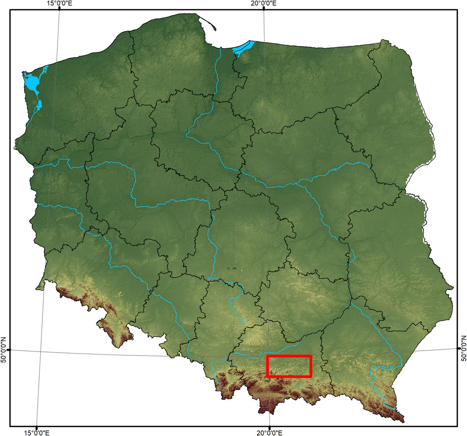
FIGURE 1. Location on the study area.

The Carpathian Foredeep is a foreland trench of the Carpathians, formed in the Neogene as a result of the Alpine orogenesis. It is filled with Miocene sediments covered by a thin, discontinuous layer of Quaternary sediments. The thickness of Miocene sediments in the foreland of the Carpathians is estimated to be between 800 and over 1,000 m (Poborski and Skoczylas-Ciszewska 1963; Połtowicz 1991). A narrow belt stretching from Wieliczka to Przemyśl contains salt-bearing sediments. Heavily folded rock salt layers are interlayered with anhydrite claystones (Bukowski 1996). The majority of the Wiśnickie Foothills area is located within the Silesian unit, a tectonic unit of the Outer Carpathians that is very differentiated stratigraphically, facially, and tectonically. The bulk of the unit is composed of outer-Carpathian flysch rocks that developed as sandstones and shales (Lower Istebna strata—Upper Cretaceous, Krosno strata—Paleogene) (Połtowicz 1974; Cieszkowski et al., 1994).

The youngest lithostratigraphic formations are Quaternary formations ranging from several to a dozen or so meters thick. They are developed mainly as fluvial deposits of valleys, slope deposits in the form of aeolian material, diluvial covers, and colluvial slope formations (Burtan 1954; Skoczylas-Ciszewska 1954; Skoczylas-Ciszewska and Burtan 1954; Burtan 1977). The slope sediments are represented by silty loess-like formations. These were formed as a result of the weathering of the Carpathian flysch and the simultaneous eolian sedimentation of loess during the Vistula glaciation. The thickness of the loess deposits in the northern part of the study area is estimated at 3–5 m, whereas the thickness of loess-like formations, silts, and sandy loams varies, ranging from 2–3 m to 6–12 m. At the foot of the slopes there are formations created as a result of denudation, flushing, washing of loess and loess-like covers. Also in the lower part of the slopes, diluvial-salifluction formations can be found, as can colluviums formed at the turn of Pleistocene and Holocene, as well as in the Holocene itself (Burtan 1954). The thickness of landslide colluviums, formed as clays, loams, and loams with debris, can reach 30 m (the Landslide Counteracting System - SOPO).

The Wiśnickie Foothills are an example of a mature fluvial-denudational sculpture, consisting of flat upland patches 350–420 m above sea level. The course of the humps and ridges reflects the main tectonic units of the Silesian unit and outcrops of more resistant bedrock. The series of the Silesian unit form large synclinal troughs, which orographically split the Foothills area into two strings of low foothills patches (relative heights 40–100 m above the valley bottom) and medium foothills (relative heights 120–250 m above the valley bottom). The foothill level, within both types of foothills, cuts and levels ridges that are composed of less resistant flysch. This level dates back to the lower Pliocene and developed in a cool and dry climate. Within the larger valleys one can find the valley level, cut to 40–60 m in relation to the height of the bottoms of modern river valleys. It consists of almost flat surfaces with a slope that does not always face in the direction of the valleys but always slopes towards their axis. This level dates back to the early Pleistocene (eopleistocene) (Starkel 1972).

The relief of the mountain ridges is dominated by long slopes with convex-concave profiles. More than 77% of the slopes fall between 2° and 15°. Moderately inclined slopes (2°–7°) occupy 38.8% of the total land area. A similar area is occupied by steeply inclined slopes (38.6%). Areas of flat ridge culminations and valley bottoms occupy 11.8% of the total. Steep slopes (15°–35°) occupy 10.7% of the area of the Foothills. The dominant orientation of the hills is northern and southern. Slopes with eastern and western exposure are less represented in the topography.

The whole area of the Wiśnickie Foothills is located in the warm temperate climate zone (Hess 1965; Obrębska-Starklowa 1977). It is characterized by an average annual air temperature of 8.3°C, with the average temperature of the coldest month (January) ranging from−3.2°C to−4.0°C, and the average temperature of the warmest month (July) ranging from 17.5 to 18.2°C (Obrębska-Starklowa 1988). According to IMGW data from the Scientific Station of the Jagiellonian University in Łazy, the average precipitation in 1989–2013 was 694.3 mm. The number of days with precipitation in this period ranged from 182 to 233. The greatest amount of precipitation occurs from May to October and constitutes 59.9%–79.8% of the annual precipitation total (the average across the entire aforementioned period was 69.5%). Precipitation during this period was characterized by high daily, monthly, and seasonal variability. Maximum daily precipitation ranged from 21 to 91.9 mm; maximum monthly precipitation ranged from 87.3 to 337 mm.

The main rivers of the Wiśnickie Foothills are right-bank tributaries of the Vistula River. 48% of the analyzed area is drained by the Raba River and its tributaries. The second largest watercourse is the Uszwica, which drains 25% of the study area. The third most important system is the Dunajec river basin, whose left-bank tributaries drain 20% of the Wiśnickie Foothills. In the northern part of the area, the Gróbka (Grabka) and Kisielina rivers represent a small share in the hydrographic system of the Foothills.

A significant part of the Wiśnickie Foothills (66%) is covered by formations with low permeability, with a permeability coefficient from 10^–5 to 10⁻⁸ m s⁻¹, represented by cohesive soils (silty and loamy sands, loams, silty and sandy loams, and silts). The remaining area is dominated by medium-permeability soils (19%) represented by sands, fluvisols, silts, and sedimentary and solid rocks that are strongly sealed. The remaining part of the Wiśnickie Foothills area consists of soils with very low permeability, lower than 10^–8 m s⁻¹, represented by clays, loams, silt loams, and fluvisols on clays. The depth of the groundwater table within the foothills varies. In the valley bottoms and within the inflow cones, they usually do not exceed 0.5–3.0 m. On the slopes and in the upper parts, the water table may range from 1 m to 6–10 m (Kleczkowski 1992).

The soil cover of the Carpathian Foothills and their structure reflect the geological substrate, the relief, the climate, and the vegetation. These conditions resulted in the development of acid brown soils and rainwater-gley soils. The conditions in large river valleys favored the formation of mud and swamp soils (Uziak 1962; Siuta and Rejman, 1963; Firek 1977; Zasoński, 1981; Skiba, 1992; Skiba and Drewnik, 1995; Skiba et al., 1995). The grain size composition of the slope formations is characterized by low sand fraction content (up to 10%), significant silt fraction content (50%–70%), and considerable clay fraction content (8%–18%) (Święchowicz 2012). About 60% of the study area is covered by complexes of loess and loess-like formations of varying thickness. The second largest land cover is a complex of medium loams (covering about 12% of the area). The greatest concentration of these is in the southern (highest) part of the area and in the west, on the hills along the Raba river valley. In the close vicinity of the heavy loams there are light loams, which occupy about 6% of the whole study area.

Detailed studies on the number and location of landslides in the Wiśnickie Foothills were carried out within the SOPO program (the Lanslide Counteracting System) coordinated by the Polish Geological Institute - National Research Institute (PIG-PIB). The program recorded over 5,000 landslides in the area. Their average density in the study area is 4.9 landslides per 1 km² (6 landslides per 1 km² of slopes). With respect to the type of slope material in which landslides are formed, the dominant types are landslides of weathered rocks on bedrock (41.3%) and deep-seated landslides (composed of rock and weathered rock—43.9%).

A closer examination of the map of landslide locations in the Wiśnickie Foothills (Figure 2B) shows a high concentration of landslides in the northern part of the study area, in the Brzeskie Foothills belt. The character of mass movements registered within the SOPO program is varied. In this study we focused on shallow landslides which were formed within slope covers, that means landslides composed of soils or those which were formed on the contact zone of soil and weathered bedrock. These landslides are almost 60% of all landslides registered within the SOPO program and they are activated usually more rapidly than deep-seated ones. Considering the forecasts of climate change, it is predicted that in the future shallow landslides will be activated more and more often in this region of Europe (Gariano and Guzetti, 2016). These landslides are present in the whole area of the Wiśnickie Foothills, primarily in its central, west-northern and western part. The average density of these landslides in the study area is 3.4 landslides per km², while the maximum density is 36 landslides per km².

FIGURE 2

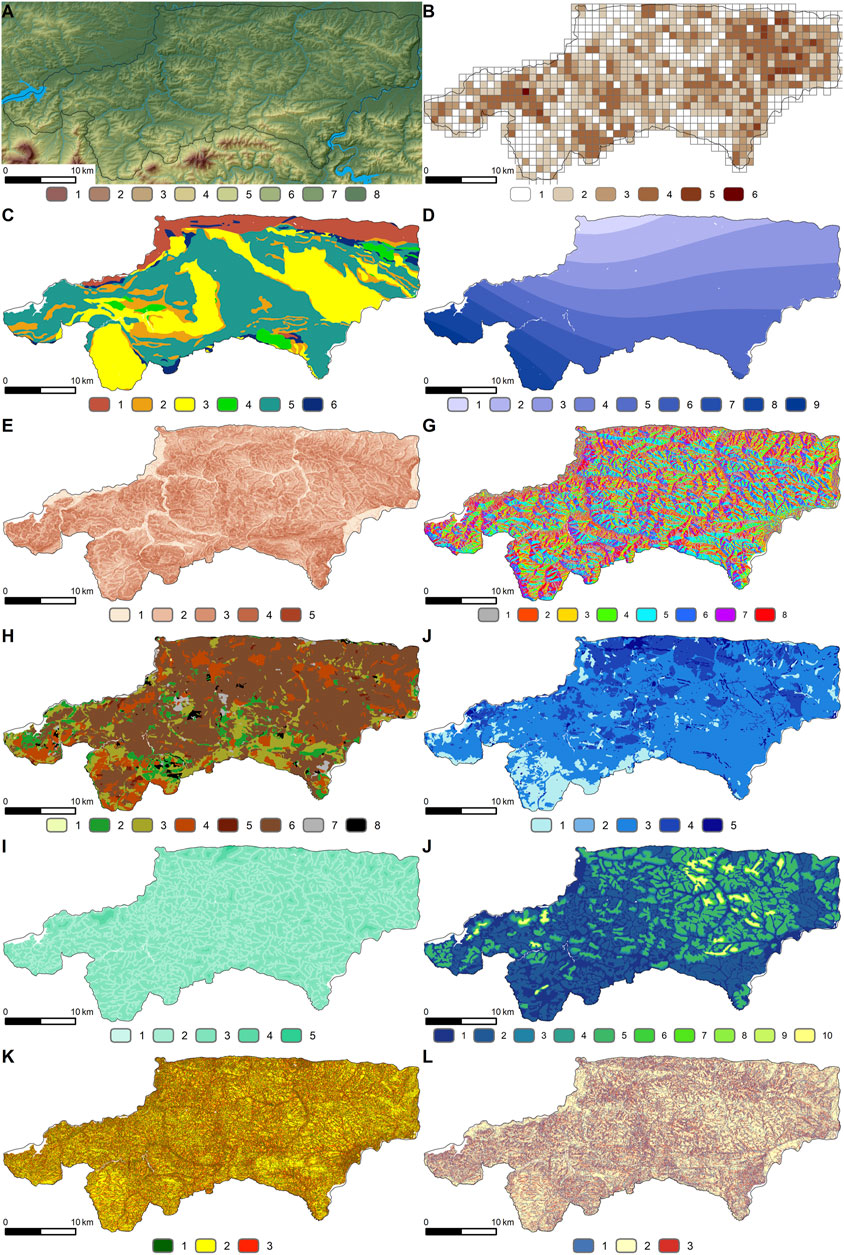
FIGURE 2. Characteristics of the analyzed area (A,B) and summary of thematic maps used in landslide susceptibility analysis (C–L): (A) Numerical terrain model [m below terrain] (1. 800–900; 2. 700–800; 3. 600–700; 4. 500–600; 5. 400–500; 6. 300–400; 7. 200–300; 8. 190–200). (B) Landslide density map (number of landslides/1 km²) (1. 0; 2. 0–2; 3. 2–5; 4. 5–15; 5. 15–30; 6. 30–45). (C) Geological map (1. siltstone, claystone, sandy siltstone, sands and sandstone (Miocene); 2. variegated shale; 3. shale and sandstone; 4. sandstone; 5. sandstone and shale; 6. other (gypsum, anhydrite, rock salt, gaize, siliceous marl, gray marl). (D) Annual precipitation [mm] (1. 675–700; 2. 700–725; 3. 725–750; 4. 750–775; 5. 775–800; 6. 800–825; 7. 825–850; 8. 850–875; 9. 875–900). (E) Slope map (degrees) (1. 0–2; 2. 2–7; 3. 7–15; 4. 15–35; 5. greater than 35). (F) Slope exposure (1. N; 2. NE; 3. E; 4. SE; 5. S; 6. SW; 7. W; 8. NW). (G) Map of soils (1. Skeletal soils; 2. Light loams; 3. Medium loams; 4. Heavy loams; 5. Clay; 6. Silt; 7. Light loamy sands; 8. Strong loamy sands). (H) Soil permeability map (1. very low permeable soils; 2. high permeable soils; 3. low permeable soils; 4. average permeable soils; 5. variably permeable soils). (I) Map of distance to rivers and streams (m) (1. 0–5; 2. 5–100; 3. 100–500; 4. 500–1,000; 5. 1,000–2,000). (J) Map of depth to groundwater (m below terrain) (1. 0–1; 2. 1–2; 3. 2–3; 4. 3–4; 5. 4–5; 6. 5–6; 7. 6–7; 8. 7–8; 9. 8–9; 10. 9–10). (K) Plan curvature map (1. ≤−0.005; 2. (−0.005–0.005>; 3. > 0.005). (L) Profile curvature map (1. ≤−0.001; 2. (−0.001–0.001>; 3. >0.001).

Shallow landslides are most common on slopes between 10° and 14° (40.6% of shallow landslides). Areas with slopes that are smaller than 10° contain 25.3% of the remaining shallow landslides. As slope increases, the number of landslides decreases. Only 6.2% of landslides are located in areas with slopes above 20°, which is due to the dynamics of denudational processes (largely flushing) in the geological past. In areas with steep slopes, which are the most predisposed to the formation of slope processes, the presence of surface runoff and surface and furrow flushing processes is more frequent; these areas are the first to achieve a state of slope equilibrium, thus reducing the risk of landslides.

Shallow landslides in the Wiśnickie Foothills mostly develop on straight (29.6% of shallow landslides), convex-concave (24.6%) and convex-convex (24.2%) slopes. On straight slopes, landslides are proportionally distributed across the slope profile. In the other types of slopes, one part clearly shows a greater proclivity for landslides. For convex-concave slopes, most landslides occurred in the upper part of the slope (39.3%). The presence of shallow landslides on a convex slope is most often associated with the lower part of the slope (32.9%) or the landslide occupies the entire length of the slope (20.7%). The only slope type with a dominant presence of shallow landslides in its central part is the concave slope, within which their 21% of shallow landslides occurred.

In the Wiśnickie Foothills, shallow landslides most often occur in the steep parts of a given slope type (e.g., lower part of convex slope, middle part of concave slope), due to their presence in the main relief elements and slope types. Their presence is also connected with the level of moisture in a given part of the slope (lower part of the slope, where springs are more abundant) and the distance from the riverbed. In the case of landslides located in the lower part and covering the whole slope profile, respectively, 23% and 25% of shallow landslides are located no farther than 1 m from the riverbed, and about 80% occur at a distance up to 100 m. Landslide activity is high on northern, north-western and north-eastern slopes in relation to the other slopes, especially those with southern and south-eastern exposure. It should be added that there are no significant differences in the inclination of slopes that face each other. The dominance of the presence of shallow landslides on the northern and north-western exposed slopes can also be observed when analyzing the ratio of the area of the landslides themselves to the total area of slopes that have the same exposure (2.0 and 2.3%, respectively). For the south and southeast slopes, these values are 1.6% and 1.0%, respectively. The proportion of shallow landslides on the other slopes does not exceed 12.1% of its total number.

The greatest number of shallow landslides within the Wiśnickie Foothills (57.8%) occurs within silts. About 30% occur within heavy or medium loams. The fourth most abundant complex in terms of shallow landslides is light loam, which accounts for 7.5%. Analyzing the ratio of the area of the landslides themselves to the total area of a given complex, we can conclude that complexes of clayey soils are the most susceptible to landslides, followed by light loams and the complex of loess formations.

Preparation of Data for Analysis

A 1 m × 1 m spatial resolution numerical terrain model developed via LiDAR from ALS flybys was used to assess landslide susceptibility of the Wiśnickie Foothills. The terrain model was aggregated to a resolution of 10 m × 10 m and a slope model and slope exposure were created based on the model. Slope curvature data (Plan and Profile Curvature) were developed in the SAGA software.

Vector data from the 1:25,000 Soil and Agricultural Map, produced by the Institute of Soil Science and Plant Cultivation - National Research Institute (IUNG) in Puławy, were used to evaluate the mechanical composition of the slope covers (soils).

Based on IMGW-PIB (Institute of Meteorology and Water Management - National Research Institute) data, we analyzed the annual precipitation totals from meteorological stations and posts in the Wiśnickie Foothills and its surroundings (1984–2013). In order to ensure that the study remained representative, only those stations that had at least 30-year-long precipitation measurement sequences were evaluated (Wojnicz, Dobczyce, Łapanów, Łazy, Borusowa, Borzęcin, Igołomia, Kraków-Balice, Limanowa, Łapanów, Maków Podhalański, Nowy Sącz, Rozdziele, Tarnów, Wadowice, Węglówka). The maps of mean annual precipitation for the Wiśnickie Foothills were based on the mean values of precipitation across time.

To statistically analyze the distribution of landslide forms in the Wiśnickie Foothills, we used the materials collected during the SOPO program (the Landslide Counteracting System). We obtained permission from the authorities of the Polish Geological Institute - National Research Institute to use data from 2021. Details included:

• location and shape of the landslide (vector data),

• the type of material in which they formed: soil landslides, weathered rock landslides on bedrock, rock landslides, rock and weathered rock landslides, and mixed landslides.

To analyze the location of landslides in the Wiśnickie Foothills area, data from the following municipalities were used:

- Dobczyce (authors: Zbigniew Koluch, Danuta Nowicka),

- Gdów (authors: Zbigniew Koluch, Danuta Nowicka),

- Bochnia (authors: Izabela Laskowicz, Bartłomiej Warmuz, Paweł Marciniec),

- Bochnia miasto (authors: Izabela Laskowicz, Bartłomiej Warmuz, Bogusław Bąk, Paweł Marciniec),

- Rzezawa (authors: Izabela Laskowicz, Bartłomiej Warmuz, Ziemowit Zimnal),

- Brzesko (authors: Dariusz Wieczorek, Andrzej Stoiński),

- Wojnicz (authors: Witold Popielski, Sławomir Kurkowski, Maciej Falkiewicz),

- Zakliczyn (authors: Leszek Jurys, Tomasz Woźniak, Anna Małka, Władysława Rudeńska, Jerzy Frydel),

- Czchów (authors: Dariusz Wieczorek, Andrzej Stoiński, Rafał Dąbrowski),

- Łososina Dolna (authors: Michał Bąk, Michał Długosz, Elżbieta Gorczyca, Krzysztof Kasina, Tomasz Kozioł, Dominika Wrońska-Wałach, Przemysław Wyderski),

- Gnojnik (authors: Jerzy Jodłowski, Jacek Puchyra, Agnieszka Winiecka),

- Iwkowa (authors: Sylwester Sydow, Piotr Dobrzański, Karolina Neczyńska),

- Lipnica Murowana (authors: Maciej Multan, Joanna Bagrowska, Tomasz Dobosz),

- Nowy Wiśnicz (authors: Mariusz Kmieciak, Łukasz Dudziak),

- Żegocina (authors: Jarosław Winnicki, Jacek Puchyra, Aleksandra Smyrak-Sikora),

- Trzciana (authors: Jarosław Winnicki, Aleksandra Smyrak-Sikora, Agnieszka Kruzel),

- Łapanów (authors: Zbigniew Koluch, Danuta Nowicka),

- Limanowa (authors: Jerzy Jodłowski, Tomasz Dobosz, Konrad Poroszewski, Agnieszka Winiecka),

- Jodłownik (authors: Bartłomiej Szałamacha, Błażej Trzmiel),

- Raciechowice (authors: Józef Boratyn, Konrad Boroń, Konrad Górka),

- Wiśniowa (authors: Bartłomiej Szałamacha, Błażej Trzmiel),

- Myślenice (authors: Józef Boratyn, Michał Bąk, Krzysztof Kasina).

Data on geological structure, rock permeability, depth to groundwater table, and distance to watercourses and rivers were derived from mapping studies such as:

• 1:10,000 topographical maps in the 1992 system and in the 1965 system,

• 1:50,000 Detailed Geological Map of Poland (sheets: Bochnia, Brzesko, Wieliczka, Mszana Dolna) and 1:200,000 map (Nowy Sącz sheet),

• 1:30,000 soil maps of Poland (sheets: Nowy Sącz, Cieszyn),

• 1:50,000 hydrographic Map of Poland (sheets: Bochnia, Brzesko, Wieliczka, Mszana Dolna, Limanowa, Łososina Dolna, Wojnicz).

Original geological map of study area contained 25 basic lithological units. The map of soils was contained over 800 unique classes, where each one contained up to five horizons. To simplify calculations and to avoid too many different data in training and testing datasets we have merged smaller units into the more generalized ones. The division of geological units into bigger ones was partly based on the criterion of classification of flysch slopes proposed by Zabuski et al., (1999) for the Outer Carpathians in Poland. In this classification lithology of an area is simplified and only includes the content of shales in rock massif. The criterion used for merging soils was the based on the soil type present in the upper horizons.

The individual thematic maps are shown in Figures 2C–2L, and the detailed relationship of each factor to landslide terrain is summarized in Figure 3.

FIGURE 3

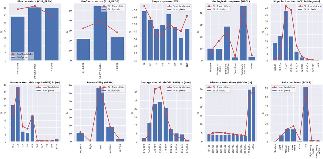
FIGURE 3. Distribution of environmental factors within analyzed area and relationship between landslides and the analyzed factors.

Methodology

Data Preprocessing

Data from ten thematic maps, one of which was a landslide map, were used in the calculations. The parameter values on each map were categorized; next, sparse matrices were created for the calculations and combined to form an input array containing binary values. Data categorization was performed using the pandas library. Prior to computation, the data was divided into training and test sets using a 70:30 ratio. Previous studies by Ng et al. (2021), Saha et al., (2021a), and others indicate that this ratio of training data to test data usually yields the best results. The scope of the analysis is shown in Figure 4.

FIGURE 4

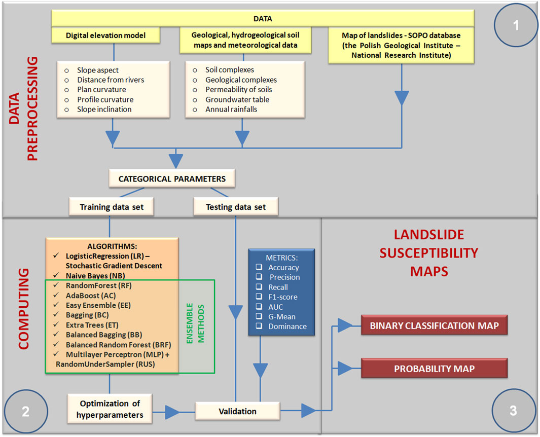
FIGURE 4. Computational procedure.

Computational Algorithms

The susceptibility of slopes to mass movements can be assessed using supervised learning methods. Given that the research question involves determining whether the area in question is susceptible to mass movements or not, this analysis is a binary classification task. There are many machine learning algorithms with a plethora of common applications to natural phenomena and processes. In this paper, the research problem we tackle represents an analysis characterized by large variation in the size of individual classes (landslides comprise about 2.0% of the Wiśnickie Foothills). The lack of balanced classes may lead the algorithm to seek to maximize metrics that describe the larger class, as it has a greater impact on the overall result. To counteract this process, at the preprocessing stage, researchers employ methods that balance individual classes (“oversampling,” “undersampling”) (He and Garcia, 2009; Sun et al., 2009; Galar et al., 2012) or adjust the values of individual class weights (Chen et al., 2010; Albon 2018). In this paper, both solutions were applied and the Scikit-Learn (Pedragosa et al., 2011) and Imbalanced-Learn (Lemaitre et al., 2017) libraries, available in the Python environment , were used for computation. Eleven computational methods (algorithms) were used in this study; their assumptions and characteristics are described below:

Logistic regression (LR). This method, much like linear regression, considers the relationship between the values of input and output parameters. The logistic function makes it possible to determine the probability of belonging to particular classes. Due to the size of the dataset (a table with more than 8.5 million records), we used the Stochastic Gradient Descent (SGD) algorithm from the Scikit-Learn module, which optimizes the results using the stochastic gradient descent method. Due to the imbalanced size of the analyzed data, the algorithm was regularized using the different values of the weights for each class (inversely proportional to class frequencies in the input data). The regularization of the model was performed using the grid method with cross-validation (GridSearchCV module) for three validation sets.

Naive Bayes (NB) classifier. This model determines the probability of event A conditional on the occurrence of event B P (A|B) given the availability of information P(B|A) and the probability of events A and B occurring. The Categorical Naive Bayes classifier is used in this paper. The cross-validated grid method (GridSearchCV module) was used to optimize the model using three validation sets, and the optimization was based on finding the optimal value of the alpha parameter and the prior probabilities of the classes.

AdaBoost (AB), Bagging (B), Random Forest (RF), and Extra Trees (ET) are ensemble methods built with several predictors, and each predictor is trained on a randomly generated subset from the learning set using the same algorithm. The AdaBoost, Bagging, and Extra Tress methods are based on the Decision Tree Classifier method; a detailed description of these algorithms can be found in Géron (2019). For the Bagging Classifier (Bootstrap Aggregating) model, an ensemble of classifiers is trained using random subsets (with returns), and the final prediction outcome is determined by the most frequently computed prediction. Random Forest, on the other hand, is a convenient and algorithm-optimized decision tree ensemble in which an ensemble of decision trees is learned on different subsets (bootstrap samples), and the final result is averaged to improve model accuracy and control model overfitting. For the Bagging model library used here, the number of features considered in finding the best tree partitioning criterion corresponds to the square root of the features used in the computation. Conversely, for the Random Forest model, it is equal to their total number. The Extra-Trees (Extremely Randomized Trees) ensemble takes into account a random subset of features during the partitioning of each Random Forest node. This generates random thresholds for each feature and consequently more random trees. Unlike the Random Forest method, Bagging and AdaBoost samples are not bootstrapped. The Extra-Trees algorithm is significantly faster than the Random Forest algorithm. By contrast, the Adaptive Boosting (AdaBoost) algorithm is a reinforcement learning algorithm in which each successive predictor attempts to correct its predecessor. In this method, each successive predictor “focuses” on the errors of the predecessor. After each prediction, the predictor’s weighted error rate and its weight are calculated, the sample weights are updated, and the next predictor is learned using the updated weights. The final result takes into account the predictions of all predictors, with the prediction following a majority vote. For the AdaBoost, Bagging, and Random Forest algorithms, the default estimator is the Decision Tree Classifier algorithm. In order to optimize it, we applied the grid method with cross-validation (GridSearchCV module) by taking different values of tree depth and using three validation sets. The gini index was used to determine the information gain. Then, having a predetermined tree depth for each algorithm, we performed the calculations and compared the classifier quality index values for the training (learning) and test sets. If the values of this parameter did not differ by more than 0.015, we concluded that the model was not overfitted. Balanced weights were used to balance the validity of the two classifiers.

Balanced Bagging (BB), RUSBoost (RB), Balanced Random Forest (BRF), and Easy Ensemble (EE) are composite (hybrid) computational methods designed to work with imbalanced datasets and are available in the Imbalanced-Learn library (Lemaitre et al., 2017). For each of these algorithms, computations are performed in two stages. The first stage involves generating a subset in which data from the dominant class are reduced (e.g., to a value corresponding to the amount of data present in the minority class, i.e., the class containing landslides). In the second stage, the subset is trained. The subset is generated (bootstrap trials without replacement) and trained repeatedly. The Balanced Bagging algorithm uses the Bagging ensemble for the purpose of training; its default estimator is the Decision Tree Classifier algorithm. Meanwhile, the Easy Ensemble algorithm is trained using the AdaBoost ensemble of predictors, and the Balanced Random Forest is the equivalent of the Random Forest algorithm from the Scikit-Learn library. Both algorithms use balanced boostrap sampling. Easy Ensemble uses samples to generate results using a boosting technique, while Balanced Random Forest trains random decision trees (Liu et al., 2009). The RUSBoost algorithm enables us to use any algorithm (the default option is the Decision Tree Classifier); this study uses Random Forest. This algorithm provides a hybrid solution in which data from the dominant class are reduced randomly using the Random Under Sampling algorithm and then subjected to learning using an arbitrary algorithm. The advantage of this solution is that it reduces computation time, while the disadvantage is that it loses information from the majority class due to the use of the boosting technique (Seiffert et al., 2010). In this model, the Random Forest Classifier was used as the learning algorithm. In the Bagging Balanced, Balanced Random Forest, and Easy Ensemble algorithms, the training set is reduced before learning and the default model is the Decision Tree Classifier. In these models, the main parameter that was optimized was maximum tree depth, and the model was considered appropriate if the difference in the classifier index value between the test set and the learning set did not exceed 0.01. In general, for all these models, after reduction, the size of the dominant class was the same as that of the smaller class.

Multi-layer Perceptron (MLP) is a neural network algorithm and is classified as a deep-learning method (Géron, 2019). This algorithm contains a hidden layer, and its output is a logistic function. In this paper, this algorithm is integrated with the Random Under Sampler algorithm from the Imbalanced Learn library. This algorithm randomly removes data from the dominant class, which helps to speed up the computation, and on the other hand avoids over-fitting the model with data from the dominant class. In this paper, different data proportions were tested between the two data classes (between 1:1 and 1:0.5—i.e., the count of the larger class was reduced to the number of pixels corresponding to the number of instances in the smaller class, or at most, the number of instances from the larger class was twice the count of the smaller class). After removing data from the dominant class, calculations were performed with the Multi-Layer Perceptron algorithm, and optimization (selection of the activation function and the regularization parameter l2) was performed using the cross-validation grid method on three validation sets.

Based on these calculations, we evaluated the impact of individual factors (parameters) on the presence of landslides. Calculations were performed in Google Colaboratory using the Scikit-learn (https://scikit-learn.org/stable/) and Imbalanced-Learn (https://imbalanced-learn.org/stable/). The Matplotlib (Hunter 2007) and Seaborn (Waskom 2011) libraries were used to visualize the results of the analyses.

In the case of linear models (e.g., logistic regression, linear support vector machines), it is important that the variables are not correlated with each other. The collinearity of the variables can cause numerical instability in the fit of the regression equation (Bruce et al., 2020). In the study, the calculations were performed for categorical data and therefore the collinearity calculations were performed using the Cramer’s V coefficient, which was determined with the use of a reseachpy (Bryant 2018) library.

Validation of Results

To accomplish to the goal of this study, we adopted a framework with two classes (landslide events) that describe different parts of the Wiśnickie Foothills from the point of view of their susceptibility to landslides:

• Class 0: the area is not exposed to mass movements, i.e., no such processes have been recorded there), and

• Class 1: the area is landslide-prone. i.e., mass movements have been recorded there, irrespective of the degree of current activity.

Comparing our results on the susceptibility of different sites to mass movements with the observation of landslide processes, four cases can be distinguished:

⁃ True Positive (TP): the predicted class (landslide event) is consistent with reality,

⁃ True Negative (TN): the classifier did not predict a Class 1 event and it does not occur in reality,

⁃ False Positive (FP), the classifier predicted a landslide event, whereas in fact it did not occur,

⁃ False Negative (FN), the classifier did not predict a landslide event, whereas in fact it did occur.

Based on the counts of each computational instance, the following metrics can be identified:

$Accuracy=\frac{TP+TN}{TP+FP+TN+FN}(1)$

$Recall=\frac{TP}{TP+FN}(2)$

$Precision=\frac{TP}{TP+FP}(3)$

$F1-score=\frac{2\cdot Recall\cdot Precision}{Recall+Precision}(4)$

$G-Mean=\sqrt{\frac{TP}{TP+FN}\cdot \frac{TN}{TN+FP}}(5)$

$Dominance=\frac{TP}{TP+FN}-\frac{TN}{FP+TN}(6)$

For analyses involving classes of varying size, the Accuracy parameter is not an appropriate metric because the effect of a smaller class (which is often more significant) on its value is much smaller than that of a larger class. An alternative to this parameter is the area under receiver operating characteristics curve (AUC) (Branco et al., 2015). The value of this parameter ranges from 0.5 to 1.0; the larger it is, the better the model.

The Recall parameter indicates how accurate the prediction of positive cases is, and the precision metric indicates what proportion of the data classified as positive cases represents the proportion of all cases classified as positive. A low precision value indicates that a lot of data classified as positive was misclassified (FP are common here). In turn, the F1-score value represents the harmonic mean of recall and precision.

The G-Mean parameter describes the geometric mean of the classifier accuracy of the two classes. This parameter is important to determine the degree to which the classifier avoids the negative class and the degree to which the positive class 1) is omitted from the analysis (Wang D et al., 2021). The Dominance value can range from −1 to 1 and describes how each class affects the overall computational performance. A value of 1 means that the ideal Accuracy value for the smaller class is achieved but all cases from the larger class are omitted (Branco et al., 2015).

Results

Correlation of the Input Data

The results of the collinearity calculations between the analyzed environmental factors are shown in Figure 5. General, it can be stated that the values of Cramer’s V coefficient are low indicating a slight association between the analyzed parameters. Only in three cases the values of the coefficient were greater than 0.2, but the majority of results were lower than 0.1.

FIGURE 5

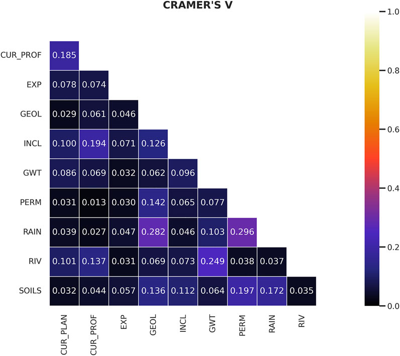
FIGURE 5. Matrix of Cramer’s V.

Model Parameters

Each model trained for an array described by 73 features. For the logistic regression (LR) model, the value of Ralph’s parameter was 0.0005 and the quotient of weights for classes 0 and 1 was 1:42.5, with a maximum number of iterations of 5,000. For the Naive Bayes (NB) classifier, the value of the additive smoothing parameter was 0.00001, with a class prior probabilities of 1.3:1 between classes 0 and 1.

For the composite models that used the Random Forest (RF) algorithm, the maximum tree depth was 15 and the number of estimators was 100. The maximum tree depth was 14 for the Bagging (B) and Extra Trees (ET) models and 6 for the AdaBoost (AB) model, with 50 estimators. The computational results showed that all estimators had an equal effect on the final result.

The hybrid algorithms had similar parameter values to their Scikit-learn counterparts. For the Balanced Bagging (BB) and Balanced Random Forest (BRF) algorithm, a maximum tree depth of 14 and 15, respectively, was used, with 60 and 100 estimators, respectively. The maximum tree depth for the Easy Ensemble (EE) model was 6, with 10 estimators. For the RUSBoost (RB) model, the AdaBoost classifier, with a maximum tree depth of 9, was used to train the model, with 10 classifiers.

For the Multi-layer Perceptron (MLP), the activation function was a logistic function, the learning speed was 0.001, with a maximum number of iterations of 2,000, a penalty coefficient of l2 = 0.0005, and a hidden layer comprising 100 neurons.

Accuracy of Models

Figure 6 shows the computational results of selected metrics for each computational algorithm. The highest Accuracy values (88.6%) for the test set were obtained by the Multi-layer Perceptron model with a 1:0.5 ratio of classes 0 and 1; the other models based on this algorithm had an accuracy of 75.7%–86.6%. For the remaining models, the RusBoost and Easy Ensemble achieved the highest value of this parameter (76.1%), while the AdaBoost model yielded a slightly lower value (74.7%). On the other hand, the Extra Trees (68.3%) and Balanced Random Forest (68.4%) models produced the lowest Accuracy (65.0%).

FIGURE 6

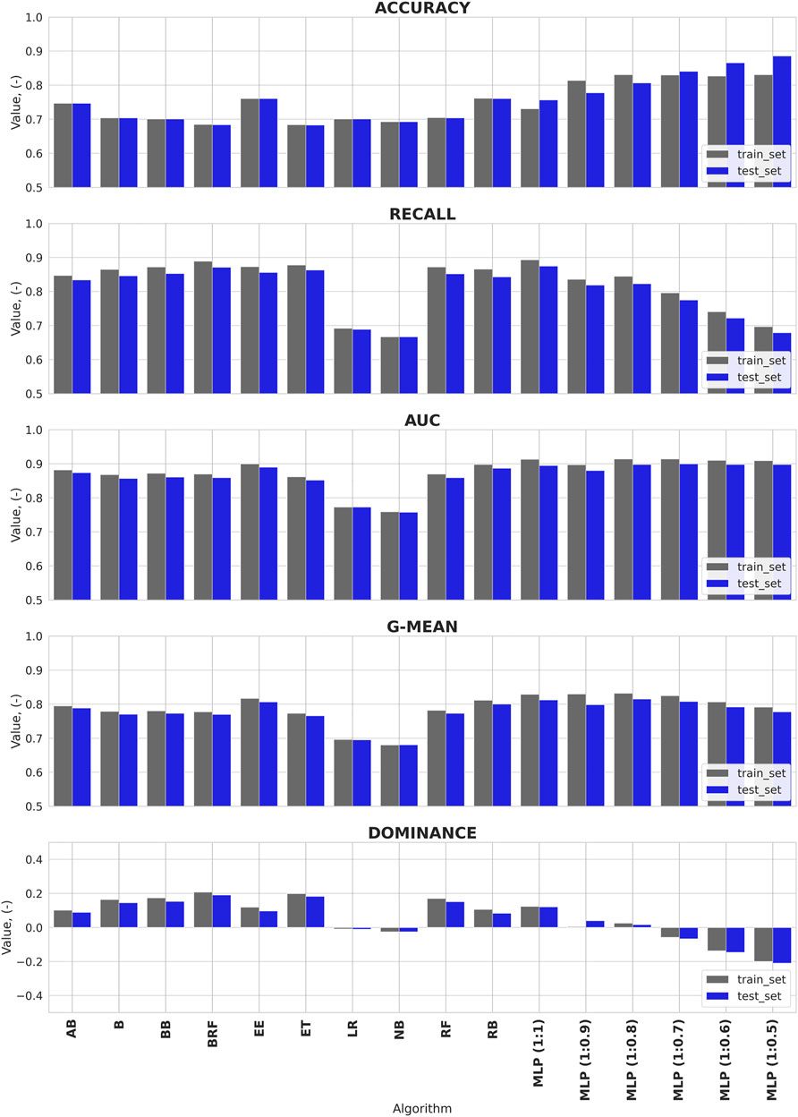
FIGURE 6. Values of metrics for each algorithm.

For the Recall parameter, the best results were obtained for the Multi-layer Perceptron models (87.5%) for the balanced dataset (MLP 1:1), with slightly poorer results for the Balanced Random Forest (87.1%), Extra Trees (86.3%), Easy Ensemble (85.6%), and Balanced Bagging (85.3%) models. By contrast, the linear algorithms yielded the lowest results, with Logistic Regression (68.9%) outperforming Naive Bayes (66.7%). Relatively poor results were obtained for Neural Network (67.9%) when the class proportions were not balanced (MLP 1:0.5).

On the other hand, the highest AUC values (Figure 7) were obtained for the neural network (88.0%–90.0%), and the results from the Easy Ensemble and RUSBoost models were very close (89.0% and 88.7%). Overall, the values of this parameter were relatively similar across the models used, which allows us to consider them serviceable (Li and He 2018). The exceptions were NaiveBayes (75.8%) and Logistic Regression (77.3%), which obtained significantly smaller values for the auc parameter.

FIGURE 7

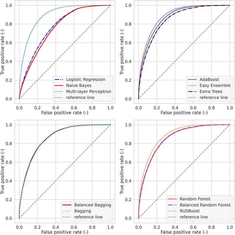
FIGURE 7. Receiver Operator Curves for the test set.

In terms of the G-Mean value (Figure 6), the algorithms that were used are of similar quality (76.6%–81.5%) except for Naive Bayes (68.0%) and Logistic Regression (69.5%). The best values of this parameter were obtained for the neural network; models based on reinforcement learning (Easy Ensemble, RUSBoost, and AdaBoost) achieved slightly lower results.

The values for the Dominance parameter (Figure 5) indicate that the neural network (except 1:1 MLP), NaiveBayes, and logistic regression do not “favor” any of the classes. For the other classes, the algorithms have parameter values between 0.08 and 0.19, indicating that the algorithms are more focused on the class 1 (the positive class, indicating the occurrence of landslide events).

The Precision and F1-score values were also considered when analyzing the computational results. Precision values are generally low and do not exceed 11%, which is due to the proportions of the classes. Only in the case of neural network, where learning was conducted for sets of the same number of classes, did the precision values reach 77.3%–78.5%, while F1-score values were at 73.3–84.1. Figure 8 presents maps of the distribution of landslide probability values generated for the algorithms used here. For the purpose of the analyses, we distinguished 5 classes of mass movement susceptibility, as proposed in Ng et al. (2021):

• Very low susceptibility (probability of site being classified as a landslide is 0%–20%),

• Low susceptibility (probability of site being classified as a landslide is 20%–40%),

• Medium susceptibility (probability of site being classified as a landslide is 40%–60%),

• High susceptibility (probability of site being classified as a landslide is 60%–80%),

• High susceptibility (probability of site being classified as a landslide is 80%–100%).

FIGURE 8

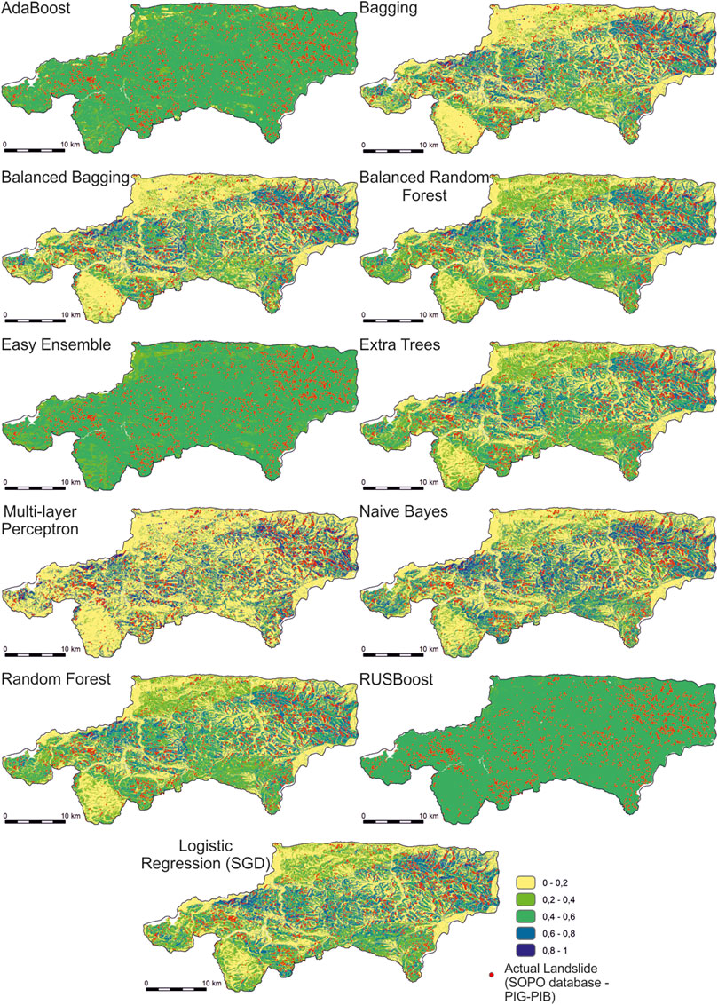
FIGURE 8. Probability distribution maps of shallow mass movements for the algorithms used.

It is clear that the AdaBoost, Easy Ensemble, and RUSBoost algorithms indicated that most of the analyzed area is located in the zone of medium susceptibility class, with the AdaBoost and Easy Ensemble models producing higher variability than RUSBoost. They also separately distinguished the presence of zones of very low and low landslide susceptibility. This type of relationship may be due to the fact that these models were characterized by lower tree depths for individual classifiers and thus may have influenced their conservative estimate of the probability value of belonging to Class 1. In the case of the other models, it is noticeable that the lowest susceptibility class occurs in the western, southwestern and northern parts of the analysis area.

The proportion of the total comprised by each susceptibility zone was compared with the number of landslides recorded (Figure 9). These results indicate that about 50%–80% of the area is at very low and low landslide susceptibility classes. It is important to note that the largest part of this area was obtained by the artificial neural network algorithm. The presence of real landslide pixels in these zones does not exceed 20% of their total number. The largest share of landslides in the very low and low landslide susceptibility class was obtained for the logistic regression algorithms, Naive Bayes, and one of the variations of the neural network (MLP 1:0.5), which was learned on the most imbalanced dataset. Except for the AdaBoost, Easy Ensemble, and RUSBoost algorithms, the proportion of areas with high and very high landslide susceptibility class does not exceed 30%, and the actual area of landslides classified in these zones ranges from 50% to 80%. The largest share of landslides in the zone of high and very high landslide susceptibility class was obtained by using the Multi-layer Perceptron algorithm, learned on a set with balanced class size. In general, for artificial neural network models in the high landslide susceptibility zone, the proportion of actual landslides is the largest. On the other hand, the models based on the decision tree algorithm—Bagging, Balanced Bagging, Balanced Random Forest, Extra Randomized Trees and Random Forest—classified the most landslides into the high landslide susceptibility zone of all the models. For the AdaBoost, Easy Ensemble, and RUSBoost models, almost the entire analysis area was classified as a medium landslide susceptibility class, which was likely due to the relatively shallow depth of the decision trees and thus the high generalizability of these models.

FIGURE 9

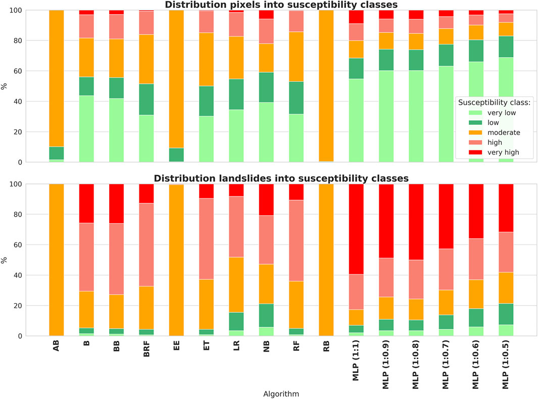
FIGURE 9. Percentage distribution of area and landslides classified in landslide susceptibility category by each algorithm.

The calculations obtained by employing neural networks provide interesting data. It is clear that, as the share of class 0 areas in the learning set increases, the share of areas with high and very high landslide susceptibility decreases and the share of actual landslide areas classified into zones with low and very low landslide susceptibility class increases. These relationships demonstrate the tendency of the algorithm to adjust itself to the dominant class.

Taking into account the results of the binary classification (Figure 10), we can conclude that 12%–33% of the Wiśnickie Foothills area is located in a zone of surface landslide susceptibility. The most optimistic analysis results were obtained for the neural network trained on the dataset with high class imbalance (MLP 1:0.5). In most cases, the size of the area exposed to shallow mass movements was between 25 and 33%, while the most pessimistic predictions were generated by Balanced Random Forest and Extra Trees methods.

FIGURE 10

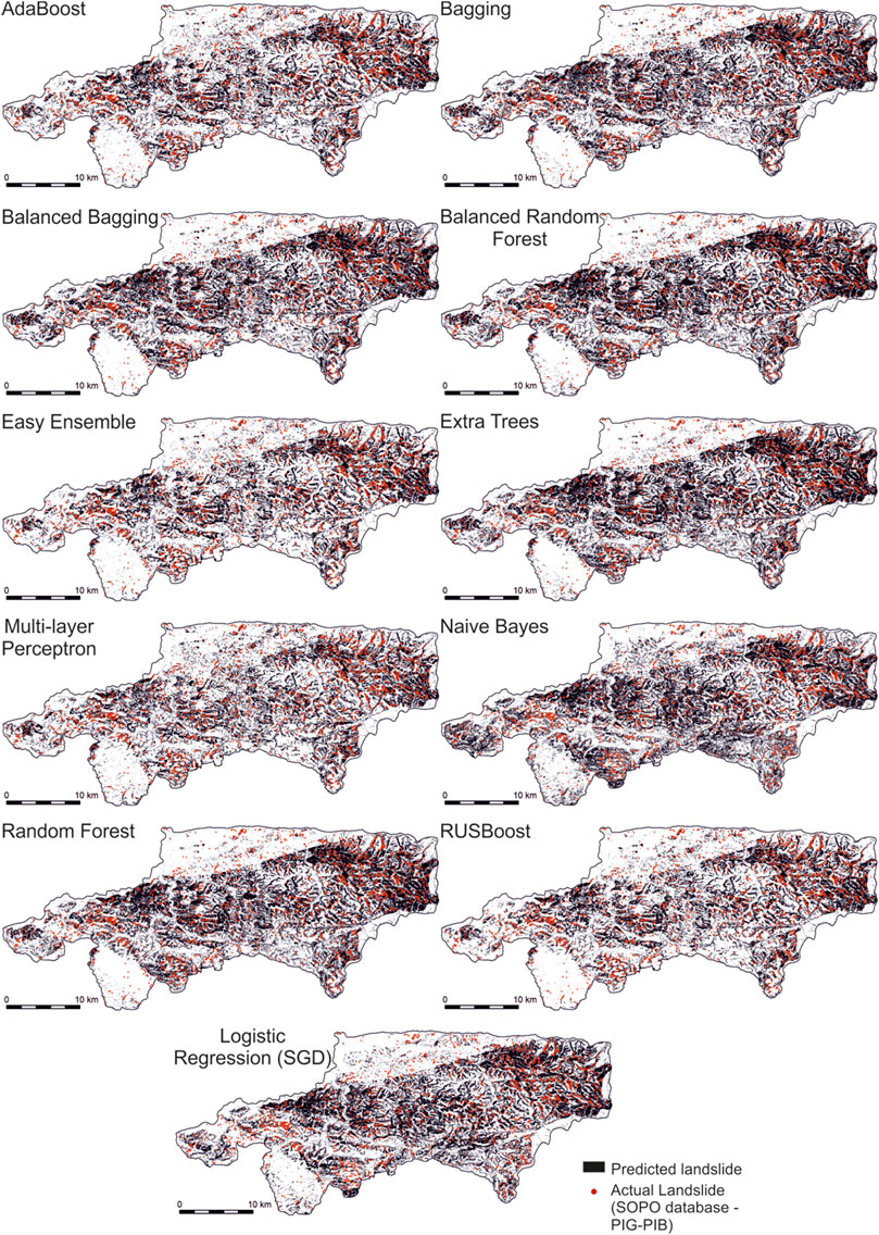
FIGURE 10. Binary classification results for the analyzed area.

Validity of Model Parameters

Supplementary Appendix S1 presents the values of model parameters for the logistic regression algorithm and the significance of parameters for models based on the decision tree method. For logistic regression, a slope inclination in the 10°–15° range, average annual precipitation of 770–775 mm, and presence of clay soils had the greatest influence on the classification results. In contrast, zones with slope inclinations between 15 and 45° are the next most important factor affecting classification.

For the Extra Trees, RandomForest, and Balanced Random Forest models, slope inclination (classes with slopes of 0°–2.5°, 2.5°–5°, 5°–10°, and 10°–15°), annual precipitation (zones with average annual rainfall in the 700–725, 725–750, and 750–775 mm ranges), and rectilinear slopes (zones characterized by profile curvature values approaching 0) were also important factors affecting the final classification.

On the other hand, in the case of AdaBoost models, the most significant factors affecting the decision were distance from rivers (more than 200 m away), the presence of shale and sandstone in the bedrock, zones with average annual precipitation of 725–750 and 750–775 mm, occurrence of heavy loams, and slope inclination (in 2.5°–5°, 5°–10° and 10°–15.0° ranges). In the case of the RUSBoost model, the most significant variables affecting the partitioning were zones with mean annual precipitation of 725–750 and 750–775 mm, areas at a large distance from rivers (more than 200 m), the presence of mixed shale-sandstone and sandstone-shale complexes, and slope inclination (zones 0°–2.5°, 2.5°–5°, and 10°–15°).

Overall, the main factors determining the classification of the analyzed area’s susceptibility to landslides are the slope inclination, rainfalls, and the presence of selected soils or rock formations.

Disscussion

Mass movements are widespread almost all over the world. Map of Europe’s landslide susceptibility based on logistic regression method (Van Den Eeckhaut et al., 2012) indicates that the area of southern Poland is characterized by an moderate susceptibility to this type of phenomena. Wojciechowski (2019) points out that the propensity of Polish lands toward landslides is usually underestimated in relation to other parts of Europe and the world. Recent efforts to map all of Poland from this perspective indicate that the Carpathian region may have experienced as many as 100,000 landslides (Wójcik and Wojciechowski, 2016), with at least 5 landslides per km². These data prove that the problem of mass movements is real. The analyzed area in the Wiśnickie Foothills belongs to the Outer Carpathians, located in the north-central part of the chain. The calculations presented in this study indicate that the environmental factors taken into account are connected to landslide risk, as evidenced by the high outcome values. In general, however, the relationship between landslide risk and the factors analyzed is complex. Therefore, linear regression or naive Bayesian classifier methods produced poorer results than methods based on decision trees and a relatively simple neural network. Logistic regression is a widely used method (e.g., Ng et al., 2021; Dai and Lee 2003; Carrara et al., 2008; Van Den Eeckhaut et al., 2012; Shou and Yang, 2015; Barella et al., 2018; Ng et al., 2021; Barančoková et al., 2021; Alqadhi et al., 2021), but its accuracy is usually lower than that of other methods. On the other hand, as indicated by Feng et al. (2016), it is more generalizable under a changing combination of factors than neural networks or the support vector method, which may indicate that it is more resistant to overfitting. The naive classifier method is not often used to determine landslide risk zones; nevertheless, the results produced by Pham et al. (2017), Barella et al. (2018), Merghadi et al. (2020) indicate that its performance is usually poor compared to other methods.

Reichenbach et al. (2018)’s review of studies on landslide susceptibility maps published in the first years of the 21st century indicates that the first decision tree-based methods appeared in the late 2000’s. Merghadi et al. (2020) demonstrate that, after 2014–2015, the popularity of ensemble models based on the decision tree algorithm increased significantly. Besides the decision tree algorithm itself (Mao et al., 2017; Guo et al., 2021; Su et al., 2021), popular variations of the method include Random Forest and Adaboost (Goetz et al., 2015; Thien Bui et al., 2016; Arabameri et al., 2017; Zhang et al., 2017; Chen et al., 2018; Hong and Liu, 2018; Lai et al., 2018; Pourghasemi and Rahmati 2018; Merghadi et al., 2020; Alqadhi et al., 2021; Saha et al., 2021a; Ng et al., 2021; Pourghasemi et al., 2021), which achieve very good prediction results in terms of accuracy and AUC values reaching or even exceeding 90%.

In this paper, a total of eight models that utilize the decision tree method were used, four of which employed the undersampling technique during learning, which speeds up the computation and also counteracts overfitting. Comparing the results of the calculations, we can conclude that the use of undersampling at the learning stage improved the prediction of most of the models. The Easy Ensemble model obtained slightly better Accuracy, Precision, Recall, and AUC values than AdaBoost. The Balanced Bagging model obtained slightly higher recall and AUC values than the Bagging model. The Balanced Random Forest model yielded lower accuracy and higher recall than the Random Forest model. Turning to the RUSBoost model, which uses the Random Forest algorithm as its primary classifier, produced higher accuracy and AUC values and lower recall than the Random Forest model. Overall, of all the methods examined here, Easy Ensemble and RUSBoost obtained the highest accuracy value, Balanced Random Forest obtained the highest recall, and Easy Ensemble and RUSBoost obtained the maximum AUC value.

These results allow us to compare the accuracy of the different approaches using composite models that rely on the decision algorithm. For the analyzed data, the AdaBoost algorithm obtained the highest Accuracy value, the Random Forest algorithm obtained the highest Recall value, and the AdaBoost algorithm achieved the highest AUC. The results presented by Thien Bui et al. (2016) showed that using the Bagging model produce better accuracy and AUC values than using reinforcement learning techniques (AdaBoost), although Hong and Liu (2018) found the inverse of this relationship. On the other hand, Ng et al. (2021) used Random Forests to obtain slightly better computational results compared to the AdaBoost model.

Despite its relatively simple design, compared to other types of neural networks (Saha et al., 2021b; He et al., 2021; Jones et al., 2021; Pham et al., 2021), the Multi-layer Perceptron algorithm is commonly used to develop landslide susceptibility maps and often performs well (Zare et al., 2018; Wang L-J et al., 2016; Wang Q. et al., 2016; Pham et al., 2017; Adnan et al., 2020; Ng et al., 2021; Polat, 2021, among others). Compared to methods that use decision trees, during learning, this model does not have the ability to adjust factor weights and adjusts to the class with more (negative) cases. For this reason, at the preprocessing stage, we applied the undersampling method using the Random under sampler algorithm. The results showed that as the size of the 0 class increases, the value of the Accuracy metric also increases, while that of the Recall metric decreases, and the effect on AUC and G-Mean can be considered negligible. After juxtaposing the high Accuracy and Recall values, we concluded that the optimal variant of the model was the one that took into account the balancing of both classes at the training stage (MLP 1:1). The results obtained with the MLP algorithm were the most favorable of all the models used. In turn, the results in Ng et al. (2021), also performed using the Scikit-Learn library, showed that the method is clearly less effective than the random forest algorithms, AdaBoost, or the support vector method.

There are several passive factors that are primarily responsible for the intensification of landslides in Poland: slopes with gradients of 9–30° (Wojciechowski 2019), the presence of tectonic dislocation zones, and flysch rocks. On the other hand, exposure and land cover bear little weight in determining the intensity of mass movements, as does the presence of buildings. Overall, Wojciechowski (2019) estimates that 15% of Poland is threatened by mass movements. A susceptibility analysis of part of the Carpathian range (near Dukla) conducted by Bronowski et al. (2016) using the Entropy Index method demonstrates that the slope and lithology of the terrain are the most important determinants of landslide occurrence. These authors also note that almost 50% of the area they analyze is characterized by very high and high landslide risk. These results are generally more pessimistic than those obtained in the present study, which may stem from the specificity of the site and the calculation method. Długosz (2011) also presents a set of landslide susceptibility analyses in the Carpathians, using the Weight of Evidence method for 4 areas. The results show that the contribution of individual factors in landslide susceptibility maps vary considerably. This analysis signaled that exposure, slope, land use, and site lithology all have a significant impact on landslide susceptibility. Bucała (2009) applied the Landslide Index method to the catchment area of Jaszcze and Jamne streams (Gorce), finding that slope inclination and land use (deforestation zones) determine surface mass movements caused by intense rainfall. Mrozek’s (2013) study of landslide susceptibility using the Weight of Evidence and Empirical Likehood Ratio methods for the environs of the town of Szymbark near Gorlice (in the Low Beskids) showed that the distance from tectonic dislocation zones, northern and eastern exposure of slopes, as well as their inclination (7°–18°) are important contributors to landslide susceptibility in the study area. The author (Mrozek 2013) also points out that including land use in the analysis of landslide potential is problematic because the rate at which humans transform the land is too high for the modern land use to correspond with the land use conditions that existed in the period when landslides were formed.

Researchers rely on different types of data to study the susceptibility of an area to landslides using machine learning techniques. In most cases, they opt for a numerical model of the terrain, which makes it possible to determine, among others, the slope, exposure, altitude, and curvature of an area, as well as data on soils present, their use, distance from roads and rivers, size of drainage basin, lithological structure, distance from tectonic faults, and precipitation. In general, the scope and preparation of parameters considered in the development of landslide susceptibility maps are not systematized, which causes the role of individual factors to change depending on the data included in the calculations.

Feng et al. (2016) showed that for artificial neural networks, depending on the adopted input dataset, the AUC parameter ranges from 70% to 87%. A separate factor sensitivity analysis conducted using Random Forest models and decision trees integrated with the logistic regression algorithm revealed that the influence of individual factors on the computational results can vary depending on the computational method used (Alqadhi et al., 2021). Goetz et al. (2015) come to similar conclusions. Thien Bui et al. (2016) note that the greatest information gain during decision tree partitioning occurs with information on distance from roads, slope, and exposure, while the lowest gain occurs in the case of distance from tectonic faults, terrain lithology, and precipitation. On the other hand, Meghadi et al. (2020) indicate that the decision tree distribution is most strongly determined by precipitation, altitude, soil type, slope, and land use, and least by slope exposure, distance from a road network, and distance from a drainage system. Wang L et al. (2021) use the maximum entropy method to posit that distance from roads, precipitation, and land use have significant effects on landslide occurrence, while distance from rivers, tectonic faults, and elevation all have a minor effect. Pham et al. (2021) turned to artificial neural networks to argue that distance from rivers, terrain curvature, elevation, and slope are important factors, but distance from rivers and Normalized Difference Vegetation Index (NDVI) do not affect the calculation results. Conversely, Yuvaraj and Dolui (2021) posit that precipitation, slope, and lithology are important in vulnerability calculations. It is interesting that the authors find that the highest intensity of landslides occurs in the subclass characterized by the lowest precipitation. Ng et al. (2021) reinforce this finding on the significant influence of precipitation on the results of the analysis but show that the single most important factor is slope inclination, whereas the geological structure of the terrain has the least influence. Shou and Yang. (2015) and Goetz et al. (2015) reaffirm the very significant effect of slope on the result of the classification.

Combining the results obtained in this study with those that emerge from the literature, we can conclude that environmental factors have a complex impact on the occurrence of landslides. Methods based on the decision tree algorithm often have the advantage of making it possible to determine the importance of individual factors on the prediction results. In this study, we showed that the important factors that influence the results of the calculation include slope of the terrain, variation in precipitation, and the presence of site-specific soils or rock formations. In general, the relationships uncovered here are consistent with existing views that slope stability is the end result of the interaction of passive factors (slope, soil type, geological structure) with active factors (precipitation, climate and meteorological conditions, land cover, anthropogenic factors). The role of individual factors in initiating mass movements in different regions may vary, which means that computational algorithms developed for one area may not be effective for others. In such situations, deterministic methods based on modeling physical processes in the soil environment are advantageous. The disadvantage of these methods, in turn, is that it is necessary to obtain detailed data on the geological structure of the area and the geotechnical properties of soils and rocks. Statistical methods, especially machine learning methods, are a cheaper and faster tool for hazard assessment and at the same time make it possible to identify a model landslide area on the basis of practically any environmental information about the area.

Conclusion

In this paper, we calculate the susceptibility of the Wiśnickie Foothills area, which is located in the northern part of the Polish Carpathians, to surface-level mass movements. We used several environmental factors (slope inclination and aspect, terrain curvature, groundwater table depth, distribution of precipitation, distance from rivers, soil complexes, permeability of slope cover, major geological complexes) in the analysis to determine their relationship with the presence of landslides using various machine learning techniques using logistic regression, the naive Bayes classifier, composite methods based on decision tree techniques, and a simple neural network (Multi-layer Perceptron). For most of the calculations, we trained the models using imbalanced datasets; we adjusted the importance of each class using weights or the undersampling technique to balance the classes.

The results of the calculations indicate that 25%–33% of the Wiśnickie Foothills is in a zone threatened by shallow mass movements. These data show that the issue of mass movements in the Wiśnickie Foothills is important in the context of ensuring the safety of its inhabitants and the provision of services that maintain the technical infrastructure in the area.

The results of the analyses indicate that the influence of the factors examined in this study on the landslide susceptibility of a given site is complex and multifaceted. Logistic regression and the naive Bayes classifier produced the least precise results. Models based on the decision tree method, were the choice of classifier depended on the metric used, generated much stronger results. In this case, given that the size of the classes is strongly imbalanced, it is reasonable to use the recall, dominance metric, while the use of the AUC metric should be preceded by an analysis of other metrics. Taking these factors into account, AdaBoost, Easy Ensemble, and RUSBoost are all useful algorithms. On the other hand, considering probability of landslide occurrence Balanced Bagging seems to be the most reasonable choice to classify the landslide susceptibility of the area among the models based of decision tree classifier. RUSBoost, Easy Ensemble and Balanced Bagging are hybrid algorithms, where in the first stage of learning, the dataset is subjected to random reduction of the set describing the majority class. The advantage of using this technique is that it reduces computation time, and repeatedly learning the model on bootstrap samples reduces model overlearning. When all metrics were taken into account, it can be stated that the best results were provided by the Multi-layer Perceptron model, which was learned on a balanced dataset.

The obtained results indicate that decision tree based algorithms and neural networks are very useful for classifying areas that are prone to mass movements. The advantage of machine learning algorithms is that they allow us to evaluate the probability of a landslide occurring in a given area while taking into account practically any number and form of parameters describing the area itself. The dynamic development of computer science increases access to data that pinpoints changes in environmental and meteorological conditions, which creates the prospect of new future applications of machine learning techniques for geohazard early warning systems.

Data Availability Statement

The original contributions presented in the study are included in the article/Supplementary Material, further inquiries can be directed to the corresponding author.

Author Contributions

Conceptualization, TZ and PD; Methodology, TZ; Software, PD and TZ; Validation, TZ; Formal analysis, TZ and AG; Investigation, PD and TZ; Data curation, TZ and PD; Writing—original draft preparation, TZ and PD; Writing—review and editing, TZ, AG, and PD; Supervision, TZ; Project administration, AG; Funding acquisition, AG and PD.

Funding

Funded by a grant from the Ministry of Education and Science to the University of Agriculture in Krakow for 2021.

Conflict of Interest

The authors declare that the research was conducted in the absence of any commercial or financial relationships that could be construed as a potential conflict of interest.

Publisher’s Note

All claims expressed in this article are solely those of the authors and do not necessarily represent those of their affiliated organizations, or those of the publisher, the editors and the reviewers. Any product that may be evaluated in this article, or claim that may be made by its manufacturer, is not guaranteed or endorsed by the publisher.

Acknowledgments

We are grateful to the Polish Geological Institute - National Research Institute (PIG-PIB) for providing data on the locations and characteristics of landslides.

Supplementary Material

The Supplementary Material for this article can be found online at: https://www.frontiersin.org/articles/10.3389/feart.2022.872192/full#supplementary-material

References

Adnan, M. S. G., Rahman, M. S., Ahmed, N., Ahmed, B., Rabbi, M. F., and Rahman, R. M. (2020). Improving Spatial Agreement in Machine Learning-Based Landslide Susceptibility Mapping. Remote Sens. 12, 3347. doi:10.3390/rs12203347

CrossRef Full Text | Google Scholar

Albon, C. (2018). Machine Learning with Python Cookbook: Practical Solutions from Preprocessing to Deep Learning. O’Reilly 366.

Google Scholar

Aleotti, P., and Chowdhury, R. (1996). Landslide Hazard Assessment: Summary Review and New Perspectives. Bull. Eng. Geol. Eng. 58, 21–44. doi:10.1007/s100640050066

CrossRef Full Text | Google Scholar

Alqadhi, S., Mallick, J., Talukdar, S., Bindajam, A. A., Van Homg, N., and Saha, T. K. (2021). Selecting Optimal Conditioning Parameters for Landslide Susceptibility: an Experimental Research on Aqabat Al-Sulbat,Saudi Arabia. Environ. Sci. Pollut. Res. doi:10.1007/s11356-021-15886-z

CrossRef Full Text | Google Scholar

Arabameri, A., Pourghasemi, H. R., and Yamani, M. (2017). Applying Different Scenarios for Landslide Spatial Modeling Using Computational Intelligence Methods. Environ. Earth Sci. 76, 832. doi:10.1007/s12665-017-7177-5

CrossRef Full Text | Google Scholar

Arnone, E., Noto, L. V., Lepore, C., and Bras, R. L. (2011). Physically-Based and Distributed Approach to Analyze Rainfall-Triggered landslides at Watershed Scale. Geomorphology 133 (3-4), 121–131. doi:10.1016/j.geomorph.2011.03.019

CrossRef Full Text | Google Scholar

Barančoková, M., Šošovička, M., Barančok, P., and Barančok, P. (2021). Predictive Modelling of Landslide Susceptibility in the Western Carpathian Flysch Zone. Land 10, 1370. doi:10.3390/land10121370

CrossRef Full Text | Google Scholar

Barella, C. F., Sobreira, F. G., and Zêzere, J. L. (2018). A Comparative Analysis of Statistical Landslide Susceptibility Mapping in the Southeast Region of Minas Gerais State, Brazil. Bull. Eng. Geol. Environ. doi:10.1007/s10064-018-1341-3

CrossRef Full Text | Google Scholar

Branco, P., Torgo, L., and Ribeiro, R. (2015). A Survey of Predictive Modelling under Imbalanced Distributions. arXiv:1505.01658

Google Scholar

Bronowski, B., Chybiorz, R., and Jura, D. (2016). Landslide Susceptibility Map Ping in the Beskid Niski Mts., Western Carpathians (Dukla Commune, Poland). Geol. Quaterly 60 (3), 586–596. doi:10.7306/gq.1275

CrossRef Full Text | Google Scholar

Bruce, P., Bruce, A., and Gedeck, P. (2020). Practical Statistics for Data Scientists: 50+ Essential Concepts Using R and Python. 2nd Edition. O’Reilly.

Google Scholar

Bryant, C. (2018). Researchpy. Available at: https://github.com/researchpy/researchpy.

Google Scholar

Bucała, A. (2009). Rola Opadów Nawalnych W Kształtowaniu Stoków I Koryt W Gorcach Na Przykładzie Zlewni Potoków Jaszcze I Jamne. Pr. Geogr. 81 (3), 399–418.

Google Scholar

Bukowski, K. (1996). Złoże Soli W Bochni. W Materiałach Z Warsztatu Analiza Basenu Trzeciorzędowego Przedkarpacia. Arch. Kraków: OK PIG.

Google Scholar

Burtan, J. (1977). Szczegółowa Mapa Geologiczna Polski W Skali 1:50 000, Arkusz Mszana Dolna. Wydawnictwa Geologiczne. Warszawa.

Google Scholar

Burtan, J. (1954). Szczegółowa Mapa Geologiczna Polski W Skali 1:50 000, Arkusz Wieliczka. Państw. Inst. Geol. Warszawa.

Google Scholar

Canli, E., Mergili, M., Thiebes, B., and Glade, T. (2018). Probabilistic Landslide Ensemble Prediction Systems: Lessons to Be Learned from Hydrology. Nat. Hazards Earth Syst. Sci. 18, 2183–2202. doi:10.5194/nhess-18-2183-2018

CrossRef Full Text | Google Scholar

Carrara, A., Crosta, G., and Frattini, P. (2008). Comparing Models of Debris-Flow Susceptibility in the Alpine Environment. Geomorphology 94, 353–378. doi:10.5194/nhess-18-2183-201810.1016/j.geomorph.2006.10.033

CrossRef Full Text | Google Scholar

Chen, W., Peng, J., Hong, H., Shahabi, H., Pradhan, B., Liu, J., et al. (2018). Landslide Susceptibility Modelling Using GIS-Based Machine Learning Techniques for Chongren County, Jiangxi Province, China. Sci. Total Environ. 626, 1121–1135. doi:10.1016/j.scitotenv.2018.01.124

PubMed Abstract | CrossRef Full Text | Google Scholar

Cieszkowski, M., Burtan, J., Ślączka, A., and Zuchiewicz, W. (1994). Szczegółowa Mapa Geologiczna Polski W Skali 1:50000, Arkusz Męcina (1018). Państwowy Instytut Geologiczny Warszawa (Opracowanie Archiwalne).

Google Scholar

Ciurleo, M., Cascini, L., and Calvello, M. (2017). A Comparison of Statistical and Deterministic Methods for Shallow Landslide Susceptibility Zoning in Clayey Soils. Eng. Geol. 223, 71–81. doi:10.1016/j.enggeo.2017.04.023

CrossRef Full Text | Google Scholar

Dai, F. C., and Lee, C. F. (2003). A Spatiotemporal Probabilistic Modelling of Storm-Induced Shallow Landsliding Using Aerial Photographs and Logistic Regression. Earth Surf. Process. Landforms 28, 527–545. doi:10.1002/esp.456

CrossRef Full Text | Google Scholar

Długosz, M. (2011). Landslide Susceptibility Assessment in the Different Regions of the Polish Carpathians. Stud. Geomorphol. Carpatho-Balcanica XLV, 45–46.

Google Scholar

Feng, H., Yu, J., Zheng, J., Tang, X., and Peng, C. (2016). Evaluation of Different Models in Rainfall-Triggered Landslide Susceptibility Mapping: A Case Study in Chunan, Southeast China. Environ. Earth Sci. 75, 1399. doi:10.1007/s12665-016-6211-3

CrossRef Full Text | Google Scholar

Firek, A. (1977). Niektóre Właściwości I Kryteria Oceny Stosunków Wodnych Gleb Pyłowych Pogórza Karapckiego. Rocz. Glebozn. 34.

Google Scholar

Galar, M., Fernandez, A., Barrenechea, E., Bustince, H., and Herrera, F. (2012). A Review on Ensembles for the Class Imbalance Problem: Bagging-, Boosting-, and Hybrid-Based Approaches. IEEE Trans. Syst. Man. Cybern. C 42 (4), 463–484. doi:10.1109/tsmcc.2011.2161285

CrossRef Full Text | Google Scholar

Gariano, S. L., and Guzzetti, F. (2016). Landslides in a Changing Climate. Earth-Science Rev. 162, 227–252. doi:10.1016/j.earscirev.2016.08.011

CrossRef Full Text | Google Scholar

Géron, A. (2019). Hands-on Machine Learning with Scikit-Learn, Keras and TensorFlow. Concepts, Tools and Techniques to Build Intelligent Systems. Beijing: O’Reilly.794

Google Scholar

Goetz, J. N., Brenning, A., Petschko, H., and Leopold, P. (2015). Evaluating Machine Learning and Statistical Prediction Techniques for Landslide Susceptibility Modeling. Comput. Geosciences 81, 1–11. doi:10.1016/j.cageo.2015.04.007

CrossRef Full Text | Google Scholar

Guo, Z., Shi, Y., Huang, F., Fan, X., and Huang, J. (2021). Landslide Susceptibility Zonation Method Based on C5.0 Decision Tree and K-Means Cluster Algorithms to Improve the Efficiency of Risk Management. Geosci. Front. 12, 101249. doi:10.1016/j.gsf.2021.101249

CrossRef Full Text | Google Scholar

Guzetti, F., Mondini, A. C., Cardinali, M., Fiorucci, F., Santangelo, M., and Chang, K-T. (2012). Landslide Inventory Maps: New Tools for an Old Problem. Earth-Scince Rev. 112, 42–66.

Google Scholar

Haibo He, H., and Garcia, E. A. (2009). Learning from Imbalanced Data. IEEE Trans. Knowl. Data Eng. 21 (9), 1263–1284. doi:10.11919/j.issn.1002-0829.21805210.1109/tkde.2008.239

CrossRef Full Text | Google Scholar

He, Y., Zhao, Z. a., Yang, W., Yan, H., Wang, W., Yao, S., et al. (2021). A Unified Network of Information Considering Superimposed Landslide Factors Sequence and Pixel Spatial Neighbourhood for Landslide Susceptibility Mapping. Int. J. Appl. Earth Observation Geoinformation 104, 102508. doi:10.1016/j.jag.2021.102508

CrossRef Full Text | Google Scholar

Hess, M. (1965). Piętra Klimatyczne W Polskich Karpatach Zachodnich. Zeszyty Naukowe UJ. Pr. Geogr. 11

Google Scholar

Hong, H., Liu, J., Bui, D. T., Pradhan, B., Acharya, T. D., Pham, B. T., et al. (2018). Landslide Susceptibility Mapping Using J48 Decision Tree with AdaBoost, Bagging and Rotation Forest Ensembles in the Guangchang Area (China). CATENA 163, 399–413. doi:10.1016/j.catena.2018.01.005

CrossRef Full Text | Google Scholar

Hunter, J. D. (2007). Matplotlib: A 2D Graphics Environment. Comput. Sci. Eng. 9, 90–95. doi:10.1109/mcse.2007.55

CrossRef Full Text | Google Scholar

Jones, S., Kasthurba, A. K., Bhagyanathan, A., and Binoy, B. V. (2021). Landslide Susceptibility Investigation for Idukki District of Kerala Using Regression Analysis and Machine Learning. Arab. J. Geosci. 14, 838. doi:10.1007/s12517-021-07156-6

CrossRef Full Text | Google Scholar

Kim, D., Im, S., Woo, C., and Woo, C. (2013). Modeling the Contribution of Trees to Shallow Landslide Development in a Steep, Forested Watershed. Ecol. Eng. 61, 658–668. doi:10.1016/j.ecoleng.2013.05.003

CrossRef Full Text | Google Scholar

Kleczkowski, A. S. (1992). “Źródła I Wahania Zwierciadła Wód Podziemnych,” in Dorzecze Górnej Wisły, Część I, Eds: Dynowska I., Maciejewski M., PWN, Warszawa-Kraków.

Google Scholar

Klimaszewski, M. (1972). Geomorfologia Polski. T. 1. PWN, Warszawa.

Google Scholar

Kondracki, J. (2009). Geografia Regionalna Polski. PWN, Warszawa.

Google Scholar

Lai, C., Chen, X., Wang, Z., Xu, C-Y., and Yang, B. (2018). Rainfall-induced Landslide Susceptibility Assessment Using Random Forest Weight at Basin Scale. Hydrology Res. 48 (4), 1–16. doi:10.2166/nh.2017.044

CrossRef Full Text | Google Scholar

Lemaitre, G., Nogueira, F., and Aridas, C. K. (2017). Imbalanced-learn A Python Toolbox to Tackle the Curse of Imbalanced Datasets in Machine Learning. J. Mach. Learn. Res. 18 (17), 1–5.

Google Scholar

Li, F., and He, H. (2018). Assessing the Accuracy of Diagnostic Tests. Shanghai Arch. Psychiatry 30 (3), 207–212. doi:10.11919/j.issn.1002-0829.218052

PubMed Abstract | CrossRef Full Text | Google Scholar

Lombardo, L., and Mai, P. M. (2018). Presenting Logistic Regression-Based Landslide Susceptibility Results. Eng. Geol. 244, 14–24. doi:10.1016/j.enggeo.2018.07.019

CrossRef Full Text | Google Scholar

Mao, Y., Zhang, M., Sun, P., and Wang, G. (2017). Landslide Susceptibility Assessment Using Uncertain Decision Tree Model in Loess Areas. Environ. Earth Sci. 76, 752. doi:10.1007/s12665-017-7095-6

CrossRef Full Text | Google Scholar

Merghadi, A., Yunus, A. P., Dou, J., Whiteley, J., ThaiPham, B., Bui, D. T., et al. (2020). Machine Learning Methods for Landslide Susceptibility Studies: A Comparative Overview of Algorithm Performance. Earth-Science Rev. 207, 103225. doi:10.1016/j.earscirev.2020.103225

CrossRef Full Text | Google Scholar

Montgomery, D. R., and Dietrich, W. E. (1994). A Physically Based Model for the Topographic Control on Shallow Landsliding. Water Resour. Res. 30 (4), 1153–1171. doi:10.1029/93wr02979

CrossRef Full Text | Google Scholar

Montrasio, L., Valentino, R., and Losi, G. L. (2011). Towards a Real-Time Susceptibility Assessment of Rainfall-Induced Shallow Landslides on a Regional Scale. Nat. Hazards Earth Syst. Sci. 11, 1927–1947. doi:10.5194/nhess-11-1927-2011

CrossRef Full Text | Google Scholar

Morrissey, M. M., Wieczorek, G. F., and Morgan, B. A. (2001). A Comparative Analysis of Hazard Models for Predicting Debris Flows in Madison County. Va. U.S. Geol. Surv. - Open-File Rep. 01-0067.

Google Scholar

Mrozek, T. (2013). Zagrożenie I Ryzyko Osuwiskowe W Rejonie Szymbarku (Beskid Niski). Państwowy Instytut Geologiczny – Państwowy Instytut Badawczy, T. 199, Warszawa.

Google Scholar

Ng, C. W. W., Yang, B., Liu, Z. Q., Kwan, J. S. H., and Chen, L. (2021). Spatiotemporal Modeling of Rainfall-Induced Landslides Using Machine Learning. Landslides. doi:10.1007/s10346-021-01662-0

CrossRef Full Text | Google Scholar

Obrębska-Starklowa, B. (1988). Klimat. in: Województwo Tarnowskie – Monografia. Ed: J. Warszyński, PAN, Kraków.

Google Scholar

Obrębska-Starklowa, B. (1977). Typologia I Regionalizacja Fenologiczno-Klimatyczna Na Przykładzie Dorzecza Górnej Wisły, [dissertation] Rozp. Habil. UJ, Kraków, 11.

Google Scholar

Oszczypko, N., Ślączka, A., and Żytko, K. (2008). Regionalizacja Tektoniczna Polski - Karpaty Zewnętrzne I Zapadlisko Przedkarpackie. Przegląd Geol. 56, 927–935.

Google Scholar

Pack, R. T., Tarboton, D. G., and Goodwin, C. N. (1999). “GIS-based Landslide Susceptibility Mapping with SINMAP,” in Proceedings of the 34th symposium on Engineering Geology and Geotechnical Engineering, Logan. Editor J. A. Bay (Utah).

Google Scholar

Pedregosa, F., Varoquaux, G., Gramfort, A., Michel, V., Thirion, B., Grisel, O., et al. (2011). Scikit-learn: Machine Learning in Python. J. Mach. Learn. Res. 12 (85), 2825–2830.

Google Scholar

Pham, B. T., Tien Bui, D., Pourghasemi, H. R., and Indra, P. (2017). Landslide Susceptibility Assessment in the Uttarakhand Area (India) Using GIS: a Comparison Study of Prediction Capability of Naïve Bayes, Multilayer Perceptron Neural Networks, and Functional Trees Methods. Theor. Appl. Climatol. 122.

Google Scholar

Pham, B. T., Van Dao, D., Acharya, T. D., Van Phong, T., Costache, R., Van Le, H., et al. (2021). Performance Assessment of Artificial Neural Network Using Chi-Square and Backward Elimination Feature Selection Methods for Landslide Susceptibility Analysis. Environ. Earth Sci. 80, 686. doi:10.1007/s12665-021-09998-5

CrossRef Full Text | Google Scholar

Poborski, J., and Skoczylas-Ciszewska, K. (1963). O Miocenie W Strefie Nasunięcia Karpackiego W Okolicy Wieliczki I Bochni (Miocene in the Zone of the Carpathian Overthrust in the Area of Wieliczka and Bochnia). Rocz. Pol. Tow. Geol. 33 (3).

Google Scholar

Polat, A. (2021). An Innovative, Fast Method for Landslide Susceptibility Mapping Using GIS-Based LSAT Toolbox. Environ. Earth Sci. 6. doi:10.1007/s12665-021-09511-y

CrossRef Full Text | Google Scholar

Połtowicz, S. (1991). Miocen Strefy Karpackiej Miedzy Wieliczką a Dębicą. Kwart. AGH Geol. 17, 19–57.R

Google Scholar

Połtowicz, S. (1974). Syntetyczne Opracowanie Geologiczno-Złożowe Utworów Miocenu Między Cieszynem a Krakowem. ZOG. Geonafta.

Google Scholar

Poprawa, D., and Rączkowski, W. (2003). Osuwiska Karpat (Carpathian landslides (southern Poland)). Przegląd Geol. 51 (8), 685–692.

Google Scholar

Pourghasemi, H. R., and Rahmati, O. (2018). Prediction of the Landslide Susceptibility: Which Algorithm, Which Precision? Catena 162, 177–192. doi:10.1016/j.catena.2017.11.022

CrossRef Full Text | Google Scholar

Pourghasemi, H. R., Sadhasivam, N., Amiri, M., Eskandari, S., and Santosh, M. (2021). Landslide Susceptibility Assessment and Mapping Using State-Of-Art Machine Learning Techniques. Nat. Hazards. doi:10.1007/s11069-021-04732-7

CrossRef Full Text | Google Scholar

Reichenbach, P., Rossi, M., Malamud, B. D., Mihir, M., and Guzzetti, F. (2018). A Review of Statistically-Based Landslide Susceptibility Models. Earth-Science Rev. 180, 60–91. doi:10.1016/j.earscirev.2018.03.001

CrossRef Full Text | Google Scholar

Saha, S., Roy, J., Pradhan, B., and Hembram, T. K. (2021a). Hybrid Ensemble Machine Learning Approaches for Landslide Susceptibility Mapping Using Different Sampling Ratios at East Sikkim Himalayan, India. Adv. Space Res. 68 (7), 2819–2840. doi:10.1016/j.asr.2021.05.018

CrossRef Full Text | Google Scholar

Saha, S., Sarkar, R., Roy, J., Hembram, T. K., Acharya, S., Thapa, G., et al. (2021b). Measuring Landslide Vulnerability Status of Chukha, Bhutan Using Deep Learning Algorithms. Sci. Rep. 11, 16374. doi:10.1038/s41598-021-95978-5

PubMed Abstract | CrossRef Full Text | Google Scholar

Seiffert, C., Khoshgoftaar, T. M., Van Hulse, J., and Napolitano, A. (2010). RUSBoost: A Hybrid Approach to Alleviating Class Imbalance. IEEE Trans. Syst. Man. Cybern. A 40 (1), 185–197. doi:10.1109/tsmca.2009.2029559

CrossRef Full Text | Google Scholar

Sheng Chen, S., Haibo He, H., and Garcia, E. A. (2010). RAMOBoost: Ranked Minority Oversampling in Boosting. IEEE Trans. Neural Netw. 21 (10), 1624–1642. doi:10.1109/tnn.2010.2066988

PubMed Abstract | CrossRef Full Text | Google Scholar

Shou, K.-J., and Yang, C.-M. (2015). Predictive Analysis of Landslide Susceptibility under Climate Change Conditions - A Study on the Chingshui River Watershed of Taiwan. Eng. Geol. 192, 46–62. doi:10.1016/j.enggeo.2015.03.012

CrossRef Full Text | Google Scholar

Siuta, J., and Rejman, M. (1963). Przyczynek Do Poznania Genezy I Składu Chemicznego Gleb Ornych Pogórza Dynowskiego. Pamiętnik Puławski 9.

Google Scholar

Skiba, S. 1992: Gleby Zlewni Starej Rzeki. Zeszyty Naukowe UJ, Prace Geograficzne, 88.

Google Scholar

Skiba, S., and Drewnik, M. (1995). Odporność Gleb Pyłowych Pogórza Wielickiego Na Degradację Chemiczną. Zesz. Nauk. UJ, Pr. Geogr. 100.

Google Scholar

Skiba, S., Drewnik, M., and Klimek, M. (1995). “Gleby Pyłowe Progu Pogórza Karpackiego Między Rabą I Uszwicą,” in Dynamika I Antropogeniczne Przeobrażenia Środowiska Przyrodniczego Progu Karpat Pomiędzy Rabą a Uszwicą. Editor L. Kaszowski (Instytut Geografii UJ, Kraków).

Google Scholar

Skoczylas-Ciszewska, K. (1954). Szczegółowa Mapa Geologiczna Polski W Skali 1:50 000, Arkusz Brzesko. Państw. Inst. Geol., Warszawa.

Google Scholar

Skoczylas-Ciszewska, K., and Burtan, J. (1954). Szczegółowa Mapa Geologiczna Polski W Skali 1:50 000, Arkusz Bochnia. Państw. Inst. Geol., Warszawa.

Google Scholar

Starkel, L. (1972). Karpaty Zewnętrzne, Geomorfologia Polski. Vol. 1, PWN, Warszawa.

Google Scholar

Su, Q., Tao, W., Mei, S., Zhang, X., Li, K., Su, X., et al. (2021). Landslide Susceptibility Zoning Using C5.0 Decision Tree, Random Forest, Support Vector Machine and Comparison of Their Performance in a Coal Mine Area. Front. Earth Sci. 9. doi:10.3389/feart.2021.781472

CrossRef Full Text | Google Scholar

Sun, Y., Wong, A. K. C., and Kamel, M. S. (2009). Classification of Imbalanced Data: A Review. Int. J. Pattern Recognit. Artif. Intell. 23 (4), 687–719. doi:10.1142/s0218001409007326

CrossRef Full Text | Google Scholar

Święchowicz, J. (2012). Rainfall Thresholds for Erosion Processes in Agricultural Catchments (Rainfall Thresholds for Erosion Processes in Agricultural Catchments). IGiGP UJ.Kraków

Google Scholar

Thien Bui, D., Ho, T-C., Pradhan, B., Pham, B-T., Nhu, V-H., and Ravhaug, I. (2016). GIS-based Modeling of Rainfall-Induced Landslides Using Data Mining-Based Functional Trees Classifier with AdaBoost, Bagging and MultiBoost Ensemble Frameworks. Environ. Earth Sci. 75, 1101. doi:10.1007/s12665-016-5919-4

CrossRef Full Text | Google Scholar

Uziak, S. (1962). Zagadnienia Typologii Niektórych Gleb Pyłowych Pogórza Karpackiego, Ann. UMCS, Sec. B, 18.

Google Scholar

Van Den Eeckhaut, M., Hervás, J., Jaedicke, C., Malet,Montanarella, J.-P. L., Montanarella, L., and Nadim, F. (2012). Statistical Modelling of Europe-wide Landslide Susceptibility Using Limited Landslide Inventory Data. Landslides 9, 357–369. doi:10.1007/s10346-011-0299-z

CrossRef Full Text | Google Scholar

Wang, D., Hao, M., Chen, S., Meng, Z., Jiang, D., and Ding, F. (2021). Assessment of Landslide Susceptibility and Risk Factors in China. Nat. Hazards. doi:10.1007/s11069-021-04812-8

CrossRef Full Text | Google Scholar

Wang, L.-J., Guo, M., Sawada, K., Lin, J., and Zhang, J. (2016a). A Comparative Study of Landslide Susceptibility Maps Using Logistic Regression, Frequency Ratio, Decision Tree, Weights of Evidence and Artificial Neural Network. Geosci. J. 20 (1), 117–136. doi:10.1007/s12303-015-0026-1

CrossRef Full Text | Google Scholar

Wang, L., Han, M., Li, X., Zhang, N., and Cheng, H. (2021). Review of Classification Methods on Unbalanced Data Sets. IEEE Access 9, 64606–64628. doi:10.1109/ACCESS.2021.3074243

CrossRef Full Text | Google Scholar

Wang, Q., Li, W., Xing, M., Wu, Y., Pei, Y., Yang, D., et al. (2016b). Landslide Susceptibility Mapping at Gongliu County, China Using Artificial Neural Network and Weight of Evidence Models. Geosci. J. 20 (5), 705–718. doi:10.1007/s12303-016-0003-3

CrossRef Full Text | Google Scholar

Waskom, M. (2021). Seaborn: Statistical Data Visualization. Joss 6 (6), 3021. doi:10.21105/joss.03021

CrossRef Full Text | Google Scholar

Wojciechowski, T. (2019). Podatność Osuwiskowa Polski (Landslide susceptibility of Poland). Przegląd Geol. 67, 320–325. doi:10.7306/2019.25

CrossRef Full Text | Google Scholar

Wójcik, A., and Wojciechowski, T. (2016). Osuwiska Jako Jeden Z Ważniejszych Elementów Zagrożeń Geologicznych W Polsce (Landslides as One of the Most Important Elements of Geological Hazards in Poland). Przegląd Geol. 64 (9), 701–709.

Google Scholar

Xu-Ying Liu, X-Y., Jianxin Wu, J., and Zhi-Hua Zhou, Z-H. (2009). Exploratory Undersampling for Class-Imbalance Learning. IEEE Trans. Syst. Man. Cybern. B 39 (2), 539–550. doi:10.1109/tsmcb.2008.2007853

CrossRef Full Text | Google Scholar

Yuvaraj, R. M., and Dolui, B. (2021). Statistical and Machine Intelligence Based Model for Landslide Susceptibility Map Ping of Nilgiri District in India. Environ. Challenges 5, 100211. doi:10.1016/j.emvc.2021.200211

CrossRef Full Text | Google Scholar

Zabuski, L., Thiel, K., and Bober, L. (1999). Osuwiska We Fliszu Karpat Polskich. Geologia-Modelowanie-Obliczanie Stateczności. Gdańsk, Poland: Wydawnictwo IBW PAN.

Google Scholar

Zare, M., Pourghasemi, H. R., Vafakhah, M., and Pradhan, B. (2018). Landslide Susceptibility Mapping at Vaz Watershed (Iran) Using an Artificial Neural Network Model: a Comparison between Multilayer Perceptron (MLP) and Radial Basic Function (RBF) Algorithms. Arabian J. Geosciences 6, 2873–2888. doi:10.1007/s12517-012-0610-x

CrossRef Full Text | Google Scholar

Zasoński, S. (1981). Główne Kierunki Glebotwórcze Na Utworach Pyłowych Pogórza Wielickiego. Część I. Ogólna Charakterystyka Gleb I Niektóre Właściwości Chemiczne. Rocz. Glebozn. 32 (2), 115–143.

Google Scholar

Zhang, K., Wu, X., Niu, R., Yang, K., and Zhao, L. (2017). The Assessment of Landslide Susceptibility Mapping Using Random Forest and Decision Tree Methods in the Three Gorges Reservoir Area, China. Environ. Earth Sci. 76, 405. doi:10.1007/s12665-017-6731-5

CrossRef Full Text | Google Scholar

Zizzioli, D., Meisina, C., Valentino, R., and Montrasio, L. (2013). Comparison between Different Approaches to Modeling Shallow Landslide Susceptibility: Case History in Oltrepo Pavese, Northern Italy. Nat. Hazards Earth Syst. Sci. 13, 559–573. doi:10.5194/nhess-13-559-2013

CrossRef Full Text | Google Scholar