Earthquake Productivity Law in a Wide Magnitude Range

1 Introduction

It has recently been found that the number of aftershocks of large earthquakes in the world and the number of direct aftershocks of earthquakes in different regions of the world, considered in a fixed magnitude range relative to the main shock, obeys an exponential distribution (Shebalin et al., 2020a; Shebalin et al., 2020b). This law, called earthquake productivity law, was established for different magnitudes of the main shocks, different ways of identifying direct aftershocks, in a wide range of parameters of the algorithm for identifying aftershocks (Shebalin et al., 2020b). The data used made it possible to consider ranges of aftershock magnitudes with a lower threshold within the range of up to 2.5 units of magnitude less than the magnitude of the main shock. A further increase in the range in the reviewed catalogs was impossible, since the entire range of considered magnitudes should be above the general completeness threshold. Therefore, an increase in the range is possible only by increasing the magnitude threshold for the main shocks, which leads to their number being too small.

The exponential shape of the distribution means that the most probable number of direct aftershocks (the mode of the distribution) is 0. This property of earthquake productivity seems so counterintuitive that testing whether this shape of the distribution persists as the range of aftershock magnitudes increases has an important independent meaning. The importance of this verification is also reinforced by the fact that the exponential form of productivity contradicts one of the key elements of the ETAS stochastic model (Ogata, 1998) widely used for modeling seismicity. It is assumed in ETAS model that the productivity of earthquakes is a function of their magnitude. Under this assumption, productivity should have the form of a Poisson distribution with a non-zero mode. The same assumption is used in stochastic methods for declustering earthquake catalogs, in particular, the method based on the ETAS model (Zhuang et al., 2002) and in the model-independent MISD method (Marsan and Lengline, 2008).

The aim of this work is to investigate whether the exponential form of the distribution of earthquake productivity will be preserved with a significant expansion of the range of aftershock magnitudes. This can only be done in a region with a dense network of seismic stations and, at the same time, a high frequency of large earthquakes. We chose the land part of Japan, where the representative magnitude for crustal earthquakes since 2000 is about 1.0, and earthquakes of magnitude 6 and above occur several times a year.

2 Methods

We follow the definition of earthquake productivity adopted by Shebalin et al. (2020b). In the earthquake flow, each event is considered as a potential “parent” of subsequent earthquakes, and vice versa, each event can have a “parent”, in which case it is considered an “offspring”. The offsprings can be interpreted as immediate aftershocks. We use the nearest neighbor scheme by Zaliapin and Ben-Zion (2013). In this scheme, each parent (triggering event) can have multiple offsprings (triggered events), but each offspring can only have one parent. The parent of a given event is determined by the minimum of the proximity function (“nearest neighbor”). The proximity function determines the extent to which “parent” and “offspring” can be considered related. In this paper, following Zaliapin and Ben-Zion (2013), we use the proximity function proposed by Baiesi and Paczuski (2004):

${\eta }_{ij}=\left\{\begin{array}{cc}{t}_{ij}{\left(r_{ij}\right)}^{d_f}10^{-b{m}_i},\hfill & t_{ij}>0,\hfill \\ +\infty ,\hfill & t_{ij}\le 0,\hfill \end{array}\right.(1)$

where t_ij = t_j − t_i is the interevent time, r_ij the spatial distance between the epicenters, m_i the magnitude of event i, d_f the fractal dimension of the epicenter distribution and b the slope of the earthquake-size distribution.

Zaliapin and Ben-Zion (2013) have shown that the distribution of the nearest neighbor proximity function usually has a bimodal distribution, in which small values correspond to related events (aftershocks, foreshocks, swarms), and large values correspond to independent events. To separate related and independent events, a threshold value for the proximity function is introduced. Zaliapin and Ben-Zion (2013) proposed to approximate this bimodal distribution by the sum of two log-normal distributions. However, in reality, the form of distribution can be more complex. Therefore, Shebalin et al. (2020b) proposed to approximate the right side of the distribution using a randomized catalog of earthquakes. We believe that the distribution of the nearest neighbor proximity function in the randomized catalog is the same as for independent events. The distribution of related events is then defined as the difference between the overall distribution and the distribution for the randomized catalog. The threshold is defined in such a way as to equalize the error rates (related events with a proximity function above the threshold and independent events with a proximity function below the threshold).

After introducing the threshold, it turns out that some of the events do not have a “parent” because the proximity to the nearest neighbor exceeds the threshold. We call such events “background”. If the proximity is below the threshold the event has a “parent”. We call such events offsprings. The productivity of an earthquake then is the number of its offsprings. Here, as in (Shebalin et al., 2020b), we will use ΔM-productivity. We count the number of offsprings of magnitude M_a ≥ M_m − ΔM, where M_m is the magnitude of the parent and M_a is the magnitude of the offspring. Note that the magnitude of the offspring may be greater than the magnitude of the parent.

The scheme used here differs from the traditional mainshock-aftershock outline, which usually assumes that aftershocks are weaker than the mainshock. Another difference is that an aftershock sequence consists of a hierarchical tree of parent-offspring sequences with several levels of hierarchy (offspring of offspring, etc.). In the traditional scheme (Zaliapin and Ben-Zion, 2013), the total number of aftershocks is calculated. We count the number of offsprings at one level of the hierarchy, which can be interpreted as direct aftershocks. In this scheme, each earthquake is characterized by its ΔM-productivity value. It makes sense to analyze the values of ΔM-productivity for earthquakes with magnitude M ≥ M_c + ΔM. In this case, the offsprings are counted above the magnitude of complete registration M_c.

3 Results

3.1 Data Preparation

In this study we use the data of the catalog of the Japan Meteorological Agency (JMA)¹. Data analysis has shown that the completeness of the catalog has improved significantly since 2000. Using the multiscale analysis of the frequency-magnitude distribution (Vorobieva et al., 2013), we have constructed a completeness magnitude map from earthquake data since 2000 with a hypocenter depth h ≤ 40 km (Figure 1). We associate ranges of smaller magnitudes with decreasing areas for data selection based on empirical relations in seismotectonics.

FIGURE 1

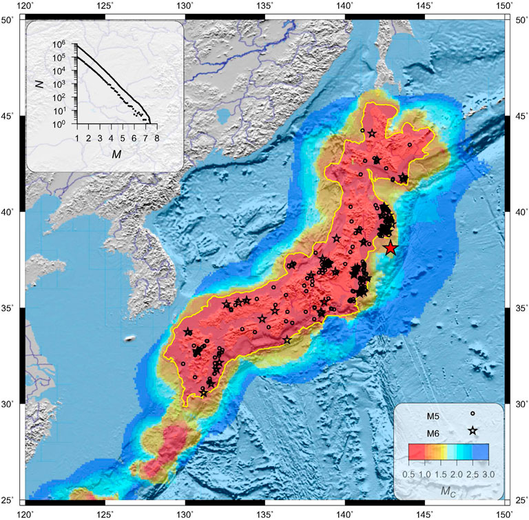
FIGURE 1. Map of the completeness magnitude M_c for the land part of Japan. The yellow line outlines the area of M_c ≤ 1. Epicenters of the earthquakes (parent events) we used in the analysis of the productivity are shown by circles (5 ≤ M < 6) and stars (M ≥ 6). Red star shows the epicenter of the Tohoku earthquake of 11 March 2011, M_w = 9.1. Tab at the top shows the frequency-magnitude distribution of earthquakes within the area of M_c ≤ 1.

The map of the completeness magnitude M_c is constructed as follows: at each point, events are selected from the magnitude intervals [M, M + W_M] in a circle with radius R(M) = 15 × 10^pM km, left end of the magnitude interval varies from 0.5 to 3. The W_M is the length of the segment of the frequency-magnitude distribution where we check a linear shape of the distribution. The exponent p has an order of b/2, that provides at a given location near-constant sample size with change of magnitude M. The radius for data selection is constant at a given magnitude segment [M, M + W_M] over the entire territory. The completeness magnitude M_c is defined as the minimum value of M for which the corresponding sample follows the Gutenberg-Richter law. This estimation is done simultaneously with the b-value estimation performed using the Bender (1983) method. The method assumes the grouping of magnitude values with a step of Δm. To decide whether the sample conforms to the Gutenberg-Richter law we check the fulfillment of the relation N₀ ≥ N₁10^(b−δ)Δm, where b is the estimate of b-value in the interval [M, M + W_M], δ is the estimated error according to Shi and Bolt (1982), N₀ number of events with magnitude m ≥ M, and N₁ number of events with magnitude m ≥ M + Δm.

High resolution of the M_c-value is achieved through the determination of the smallest space-magnitude scale in which the Gutenberg-Richter law is verified. The multiscale procedure isolates the magnitude range that meets the best local seismicity and local record capacity. Here we use the values of the parameters W_M = 1, p = 0.4, the minimum number of events in the sample is 100. The resulting value M_c is assigned to the centers of the circles located on a grid of 0.1 × 0.1°.

For further analysis, we chose the M_c = 1 completeness level (yellow outline in Figure 1). The coordinates of the nodes of this contour are given in Supplementary Table S1. The M_c ≥ 1 region closely matches the M_c ≥ 1.7 completeness magnitude region found by the JMA for the whole period in the earthquake catalog. The M_c ≥ 1 region closely matches the M_c ≥ 1.7 completeness magnitude region declared by the JMA for the earthquakes with focal depth h ≤ 150 km². The difference in M_c estimates is explained by the difference in focal depth of earthquakes. The level of registration is better for the most shallow seismicity h ≤ 40 km, which we use in our study.

4 Study of Earthquake Productivity in Land Part of Japan

For the territory under consideration, estimates were made of the values of the proximity function parameters (1): b = 0.86, d_f = 1.68 and log₁₀η₀ = −1.46. b-value is determined by Bender (1983) method in magnitude interval m ≥ 3; d_f is determined by Grassberger (1983) method also for events of magnitude m ≥ 3. The η₀ threshold was determined using the method from (Shebalin et al., 2020b). To avoid the possible influence of the Tohoku earthquake on 11 March 2011 with M = 9.1, all three parameters were estimated using data for 2000–2010.

For each earthquake with M_m ≥ 6.0, we calculated the productivity: the number of offsprings with magnitude M_a ≥ M_m − ΔM, ΔM = 5. It turned out that 39,464 triggered events were associated with 56 parent events. The frequency-productivity graph is shown in Figure 2. This plot is similar to the commonly used frequency-magnitude cumulative graph, in which frequencies are summed starting at higher values. The rectilinear form of the graph, as in the case of the Gutenberg-Richter law, indicates the exponential form of the distribution. The difference is that the productivity of each earthquake is an integer, so the resulting distribution is more correctly interpreted as a geometric distribution, for which the cumulative frequency plot, starting from large values of the argument, also has a linear form on a logarithmic scale. The slope of the graph is uniquely related to a single distribution parameter.

FIGURE 2

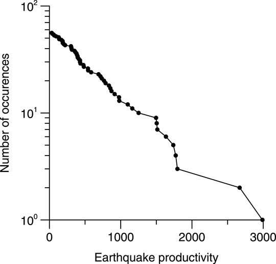
FIGURE 2. Cumulative frequency-productivity graphs for parent earthquakes with M_m ≥ 6 and offspring events with M_a ≥ M_m − 5.

Thus, we may conclude that the exponential form of the distribution of ΔM-earthquake productivity established by Shebalin et al. (2020b) for ΔM ≤ 2.5 is also confirmed for a very large range of magnitudes for ΔM = 5.

In the presented analysis, the earthquake productivity was not separated according to different levels of the hierarchy due to small number of M_m ≥ 6.0 events. Using worlwide stastistics of productivity, it was shown by Shebalin et al. (2020b) that the exponential form of the distribution and the value of its parameter change little for different levels of the hierarchy. It is this observation that gave grounds to simultaneously analyze the productivity of all earthquakes, regardless of whether they are main shocks or aftershocks in the traditional terminology. We repeated this check for earthquakes of the land part of Japan with M_m ≥ 5.0 and ΔM = 4. This property is maintained: for at least eight levels of the hierarchy, starting with background events (hierarchy level 0), the frequency-productivity plots remain linear on a logarithmic scale and have approximately the same slope (Figure 3).

FIGURE 3

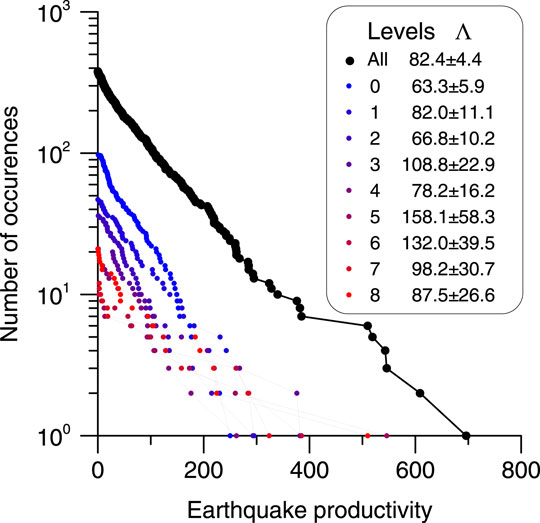
FIGURE 3. Cumulative frequency-productivity graphs for parent earthquakes with M_m ≥ 5 and offspring events with M_a ≥ M_m − 4: all earthquakes and separately for 8 highest hierarchy levels. Tab at the top shows the estimates of Λ₄ and its standard errors calculated by bootstrap method.

We verified whether the observed exponential distribution of productivity is a property of the data, or, alternatively, the result of the choice of the proximity function. We selected only background earthquakes (events of the hierarchy level 0) from the catalog and, assuming η₀ = ∞, repeated the procedure for finding for each event its parent (the closest neighbor) and calculated the productivity. The resulting distribution of the productivity of background earthquakes has a pronounced non-zero maximum (Figure 4) and, thus, is not geometric. Comparison of the distributions for background and clustered seismicity demonstrates completely different spatiotemporal structure. Thus, it is confirmed that the exponential form of the productivity distribution is a property of clustered seismicity.

FIGURE 4

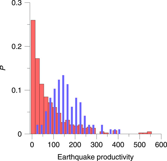
FIGURE 4. Productivity distribution for background events (blue histogram) compared to productivity distribution for clustered events (red histogram).

5 Discussion

The main result obtained here—the exponential form of the distribution of the ΔM-productivity of earthquakes [the productivity law (Shebalin et al., 2020b)] is preserved even at a very large value of ΔM. The density of the geometric distribution—an integer version of the exponential one—has a maximum value at 0. This makes this form of distribution counterintuitive. It is difficult to imagine that the most probable number of direct aftershocks is 0. It is even more difficult to believe this when direct aftershocks are considered, the magnitude of which is 5 units less than the magnitude of the earthquakes that caused them. Our analysis, however, shows that this is possible, and it becomes clear why the productivity law can remain valid even for large ΔM. The point is that for large magnitude ranges under consideration, the total number of offsprings is orders of magnitude greater than the number of parent earthquakes. In the considered example (Figure 2), with M_m ≥ 6 and Δ_M = 5, the productivity reaches 3,000, but the total number of parent events is only 56. Under these conditions, the probability of realizing the productivity value exactly 0 is small: p = 0.0014, and expected number of such earthquakes is 0.08, e.g., zero, because number of earthquakes is integer. Nevertheless, the smallest productivity values still predominate. If the number of analyzed events is much greater than the average productivity, then the number of events without direct aftershocks (productivity 0) is indeed large compared to the number of events of any other productivity (see Supplementary Material).

It is usually assumed that the productivity of earthquakes depends mainly on their magnitude. This, in particular, is used in the ETAS (Zhuang et al., 2002) and MISD (Marsan and Lengline, 2008) stochastic declustering methods. The expected ΔM-productivity distribution for such models is a Poisson distribution having a pronounced non-zero mode, this is actually predefined in these models. However, Shebalin et al. (2020b) showed, and here it is confirmed for large values of ΔM, that in reality this distribution is rather a monotone geometric one with a mode at 0. This gives additional advantages to the Zaliapin and Ben-Zion (2013) declustering method, which does not use any specified assumption. The spatiotemporal version of the ETAS model (Ogata, 1998; Zhuang et al., 2002) is also often used for seismicity modeling. The Poisson productivity distribution embedded in the model contradicts the observations. The earthquake productivity law confirmed here makes it possible to correct the ETAS model.

In a nearest neighbor schema, each parent can have multiple offsprings, but each offspring can only have one parent. This makes the productivity averaging procedure meaningful, since in such a procedure each offspring is taken into account only once. We have also shown that productivity depends little on the level of the hierarchy. This means that there is no need to distinguish between main shocks and aftershocks during averaging. ΔM-productivity averaged over some space-time region, we call after Shebalin et al. (2020b) the clustering factor. Note that in ETAS model the clustering factor is called a branching ratio. It should be less than 1 to avoid diverging aftershocks occurrence rate (Helmstetter and Sornette, 2002). For large ΔM we obtain clustering factor much larger than 1. But there is no apparent contradiction here, because the ETAS model assumes a strong relationship between the number of direct aftershocks and the main shock magnitude (Helmstetter, 2003), which was refuted by Shebalin et al. (2020b) and here again. In ΔM-analysis, the number of offsprings turns out to be weakly dependent on the magnitude of the parent, and its statistical distribution has exponential form with clear maximum at 0. This explains why large values of the clustering factor do not cause a diverging aftershock sequence. Of course, if we consider all offsprings with magnitudes above a certain threshold, their number increases with the magnitude of the parent. But this is controlled by Gutenberg-Richter law.

ΔM-productivity, similar manner to magnitude, can be seen as a property inherent in every earthquake. In this case, this value does not have to be an integer. Let’s denote this value λ. The observed value in this case is the concrete realization of the “potential” productivity of λ. It can be assumed that a particular sample is a Poisson random variable with rate λ. One more assumption can be made: the parameter λ of earthquakes, similarly to the magnitude, has an exponential distribution of the form:

$p_e\left(\lambda \right)=\frac{1}{{\mathrm{\Lambda }}_{\mathrm{\Delta }M}}\exp \left(-\frac{\lambda }{{\mathrm{\Lambda }}_{\mathrm{\Delta }M}}\right),(2)$

where Λ_ΔM is a parameter.

It is easy to show (Shebalin et al., 2020b) that the distribution of a sample of the productivity of an arbitrary earthquake in this case has the form of a geometric distribution. The estimate of the parameter Λ_ΔM is the average value of λ over the ensemble. Thus, the clustering factor has the meaning of the Λ_ΔM parameter and its estimate. The clustering factor is a convenient and a simple parameter to characterize the productivity in a set of earthquakes, for example, earthquakes in a certain space-time volume.

Data Availability Statement

Publicly available datasets were analyzed in this study. This data can be found here: https://www.data.jma.go.jp/svd/eqev/data/bulletin/index_e.html.

Author Contributions

All authors listed have made a substantial, direct, and intellectual contribution to the work and approved it for publication.

Funding

The study was supported by a grant from the Russian Science Foundation (project No. 20-17-00180).

Conflict of Interest

The authors declare that the research was conducted in the absence of any commercial or financial relationships that could be construed as a potential conflict of interest.

Publisher’s Note

All claims expressed in this article are solely those of the authors and do not necessarily represent those of their affiliated organizations, or those of the publisher, the editors, and the reviewers. Any product that may be evaluated in this article, or claim that may be made by its manufacturer, is not guaranteed or endorsed by the publisher.

Acknowledgments

The authors thank the Japan Meteorological Agency for providing the Seismological Bulletin of Japan.

Supplementary Material

The Supplementary Material for this article can be found online at: https://www.frontiersin.org/articles/10.3389/feart.2022.881425/full#supplementary-material

Footnotes

¹Japan Meteorological Agency, The Seismological Bulletin of Japan. (2022). https://www.data.jma.go.jp/svd/eqev/data/bulletin/index_e.html (Accessed 10 January 2022).

²Japan Meteorological Agency, User’s guide for The Seismological Bulletin of Japan. (2022) https://www.data.jma.go.jp/svd/eqev/data/bulletin/catalog/notes_e.html (Accessed 10 January 2022).

References

Baiesi, M., and Paczuski, M. (2004). Scale-free Networks of Earthquakes and Aftershocks. Phys. Rev. E 69, 066106. doi:10.1103/PhysRevE.69.066106

PubMed Abstract | CrossRef Full Text | Google Scholar

Bender, B. (1983). Maximum Likelihood Estimation of b Values for Magnitude Grouped Data. Bull. Seismol. Soc. Am. 73, 831–851. doi:10.1785/BSSA0730030831

CrossRef Full Text | Google Scholar

Grassberger, P. (1983). Generalized Dimensions of Strange Attractors. Phys. Lett. A 97, 227–230. doi:10.1016/0375-9601(83)90753-3

CrossRef Full Text | Google Scholar

Helmstetter, A. (2003). Is Earthquake Triggering Driven by Small Earthquakes? Phys. Rev. Lett. 91, 058501. doi:10.1103/PhysRevLett.91.058501

PubMed Abstract | CrossRef Full Text | Google Scholar

Helmstetter, A., and Sornette, D. (2002). Diffusion of Epicenters of Earthquake Aftershocks, Omori's Law, and Generalized Continuous-Time Random Walk Models. Phys. Rev. E 66, 061104. doi:10.1103/PhysRevE.66.061104

CrossRef Full Text | Google Scholar

Marsan, D., and Lengliné, O. (2008). Extending Earthquakes' Reach through Cascading. Science 319, 1076–1079. doi:10.1126/science.1148783

PubMed Abstract | CrossRef Full Text | Google Scholar

Ogata, Y. (1998). Space-time Point-Process Models for Earthquake Occurrences. Ann. Inst. Stat. Math. 50, 379–402. doi:10.1023/A:1003403601725

CrossRef Full Text | Google Scholar

Shebalin, P. N., Baranov, S. V., and Dzeboev, B. A. (2018a). The Law of the Repeatability of the Number of Aftershocks. Dokl. Earth Sc. 481, 963–966. doi:10.1134/S1028334X18070280

CrossRef Full Text | Google Scholar

Shebalin, P. N., Narteau, C., and Baranov, S. V. (2020b). Earthquake Productivity Law. Geophys. J. Int. 222, 1264–1269. doi:10.1093/gji/ggaa252

CrossRef Full Text | Google Scholar

Shi, Y., and Bolt, B. A. (1982). The Standard Error of the Magnitude-Frequency b Value. Bull. Seismol. Soc. Am. 72, 1677–1687. doi:10.1785/BSSA0720051677

CrossRef Full Text | Google Scholar

Vorobieva, I., Narteau, C., Shebalin, P., Beauducel, F., Nercessian, A., Clouard, V., et al. (2013). Multiscale Mapping of Completeness Magnitude of Earthquake Catalogs. Bull. Seismol. Soc. Am. 103, 2188–2202. doi:10.1785/0120120132

CrossRef Full Text | Google Scholar

Zaliapin, I., and Ben-Zion, Y. (2013). Earthquake Clusters in Southern California I: Identification and Stability. J. Geophys. Res. Solid Earth 118, 2847–2864. doi:10.1002/jgrb.50179

CrossRef Full Text | Google Scholar

Zhuang, J., Ogata, Y., and Vere-Jones, D. (2002). Stochastic Declustering of Space-Time Earthquake Occurrences. J. Am. Stat. Assoc. 97, 369–380. doi:10.1198/016214502760046925

CrossRef Full Text | Google Scholar