Applications of Image-Based Computer Vision for Remote Surveillance of Slope Instability

1 Introduction

Numerous monitoring approaches, including ground-based radar (e.g., Rosenblad et al., 2015), InSAR (e.g., Ferretti et al., 2007; Ferretti, 2014), Lidar (e.g., Lin et al., 2013; Tortini et al., 2015; Kromer et al., 2017; Williams et al., 2018; Williams et al., 2019; Holst et al., 2021), seismometers (e.g., Suriñach et al., 2005), and more recently computer vision (O’Donovan, 2005; Zach et al., 2007; Wedel et al., 2009; Javier et al., 2013; Sánchez Pérez et al., 2013; Kim et al., 2020; Hermle et al., 2022), have been used to study landslides and slope instability. However, the elevated cost, complexity, and intrinsic technical limitations of these methods frequently necessitates the development of alternative and complementary techniques.

At the regional scale, due to its ability to measure sub-millimetre deformation over large areas, InSAR has become one of the most powerful remote sensing monitoring techniques. However, a technical limitation is the restricted detection of measurement points over steep slopes as InSAR measures deformation along the line of sight (LOS) relative to the satellite orbit (i.e., ascending or descending) (Ferretti, 2014). In the case of more detailed and real-time monitoring of targeted mountain slopes, ground-based Radar, and Lidar (Kromer et al., 2017) can provide high resolution slope deformation monitoring (e.g., Tarchi, 2003; Vallee, 2019), but the relatively high operational costs of such techniques often limit their implementation, particularly in isolated areas with rugged topography. Hence, introducing a lower cost technique comparable to ground-based Lidar and Radar is of great interest.

Geophysical tools such as seismometers and infrasound sensors can also record signals generated by rockfalls and landslides. However, the applicability of such techniques strongly depends on the quality of the recording network, magnitude of the events, and the presence of technical expertise to properly interpretate the signals. An important limitation of these sensors is their inability to forecast landslides and rockfalls before their occurrence (e.g., Zimmer and Sitar, 2015; Ulivieri et al., 2020). Recently, a number of studies have been undertaken using computer vision codes and surveillance video cameras to forecast landslides (Amaki et al., 2019) and monitor and assess rockfalls (Kim et al., 2020); they have mainly focused on processing video frames with very short time lapse sequences. In remote and rugged mountainous areas, the challenges of providing both sufficient power and an effective means of transmitting continuous video, limits the use of real-time video datasets. These power and telemetry challenges can be addressed by collecting and processing daily static images with longer time-intervals (from hours to daily) while still enabling continuous monitoring.

In this paper, we provide an improved methodology for the application of computer vision in landslide and rockfall monitoring. The newly developed open access Python-based software, Akh-Defo (available via GitHub repository), uses optical flow velocity, image differencing and similarity index map techniques (Kim et al., 2020) to calculate land deformation (land displacement and rock fall) from a triplet of images (ground-based and satellite). Stacking of the processed triple image sets allows us to calculate the average displacement velocity over an extended period of time. Here, Akh-Defo is applied to two different datasets in British Columbia (BC), Canada and in California, United States of America (USA). The datasets include: 1) Ground-based camera images, with hourly to daily acquisitions, collected during the summer 2021 for the Plinth Peak slope of the Mount Meager Volcanic Complex (MMVC) in BC (Figure 1); and 2) Daily orthorectified satellite images, provided by Planet Labs, for the Plinth Peak slope (July 28–13 August 2021) and the 20 May 2017, Mud Creek Landslide in California (April 5–31 May 2017) (Figure 1).

FIGURE 1

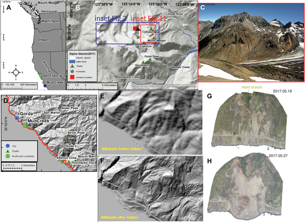
FIGURE 1. Location of the study areas. (A) Regional basemap showing the locations of Mount Meager and Mud Creek relative to western North America. (B) Hillshade map showing the location of important peaks, fumaroles, and installed camera station in the MMVC; the red inset represents the approximate area captured by the installed camera; the red square with black arrow indicates location and orientation of the camera view; the blue inset shows the area of Figure 2. (C) Example of optical image on 10 August 2021, captured at 11 a.m. by the camera station. (D) Hillshade map show location of Mud Creek landslide and the surrounding mountain peaks. (E) Hillshade map showing the topography of the Mud Creek area before the failure. (F) Hillshade map showing the topography of the Mud Creek area after the failure. (G) Oblique aerial view of Mud Creek 1 day before the failure derived from a photogrammetry model (after Warrick, et al., 2019). (H) Oblique aerial view of Mud Creek 7 days after the failure derived from a photogrammetry model (after Warrick, et al., 2019).

1.1 Research Objectives

This work has two main objectives:

1) Test whether the Akh-Defo software can complement InSAR LOS limitations via processing of ground-based optical imagery to identify rockfalls and measure land displacement in steep-slope terrain. To achieve this, we chose to apply Akh-Defo on the Plinth Peak slope of MMVC due to the presence of steep slopes and the rugged alpine mountain setting. Independent multi-temporal radar imagery processed by TRE-Altamira scientists using SqueeSAR software (Ferretti et al., 2011) provides high precision measurements of ground displacement for validation.

2) Test whether the Akh-Defo software applied to satellite optical images can identify ground displacement in active landslide regions a few weeks to months prior to initiation of landslides. To achieve this, we investigate the 20 May 2017, Mud Creek catastrophic landslide which has been very well studied and includes very high-resolution pre-, syn-, and post-landslide Lidar and photogrammetry digital surface elevation datasets (Warrick et al., 2019 and references therein).

2 Site Overview

2.1 Plinth Peak Slope, Mount Meager

The slope of interest is located on the NNW flank of the MMVC in the Garibaldi Volcanic Belt of British Columbia, Canada, an area characterized by temperate rainforests, alpine glaciers, and recently observed volcanic fumaroles. The topography consists of steep, highly altered, and unstable volcanic rock slopes which are at least partially covered with snow; visibility is often limited due to fog or low-lying cloud (Figure 1). The MMVC consists of overlapping volcanoes with a protracted history of basaltic to rhyodacitic volcanism generating lava flows and domes, pyroclastic deposits, and associated rock avalanche deposits from >1.9 Ma to present; these sit on Triassic to Tertiary Coastal Plutonic Complex intrusions and metasedimentary units (e.g., Read, 1990; Russell et al., 2021). The MMVC has erupted explosively at least twice in the past 25,000 years with the most recent event in 2360 B.P. (Russell et al., 2021); pyroclastic density currents from these eruptions were sourced at high elevation near the present-day Plinth Peak and since 2016, low level fumarolic degassing has been observed through glaciovolcanic caves on the west flank of Plinth Peak (e.g., Warwick et al., 2022).

The most recent and largest historic landslide in Canada occurred during the summer 2010 from the southern flank of Mount Meager; less than 3 km South of the current study area (Mokievsky-Zubok, 1977; Guthrie et al., 2012; Hetherington, 2014; Roberti et al., 2017; Roberti et al., 2018). Previous remote sensing and geomorphologic studies of the MMVC indicate that it hosts numerous historical and recent landslide deposits and numerous unstable areas have been identified, many of which are believed to be susceptible to future landslide events (e.g., Mokievsky-Zubok, 1977; Friele and Clague, 2004; Guthrie et al., 2012; Roberti et al., 2017; Roberti et al., 2018; Roberti et al., 2021). Hetherington (2014 and references therein) identify unstable areas on the western side of Plinth Peak and note that the eastern flank appears to have a very low factor of safety that can be presumed to be at the point of failure. The failure surface is described as being deep (Hetherington, 2014; Roberti, 2018; Roberti et al., 2021) such that should a landslide occur in this location, a major bulk of Plinth Peak could fail. Consequently, as with the 2010 landslide, it could dam the Lillooet River and cause widespread flooding downstream.

2.2 Mud Creek Landslide

The Mud Creek Landslide is located between Monterey and Morro Bay on the Big Sur coast of California, USA (Figure 1). Geomorphologically, Mud Creek coincides with the rugged Big Sur coast at the western edge of the Santa Lucia Mountains. This area includes numerous peaks higher than 1,000 m elevation, many of which are located less than 10 km from the coast. Geologically, the Mud Creek and surrounding mountain bedrock is composed of Mesozoic granitic and pre-Cretaceous metamorphic rocks, Miocene marine sedimentary rocks, and heterogeneous Mesozoic rocks which form the Franciscan Assemblage mélange overlying unconsolidated colluvial deposits (Warrick et al., 2019). Structurally, these rugged mountains are related to the Big Sur Bend of the San Gregorio-Hosgri fault system, a region of transpression along the region’s transform plate boundary (Warrick et al., 2019). This coastal mountain landslide is in an active landslide region, with coastal retreat rates during the 20th century averaging ∼0.3 m/year (Warrick et al., 2019).

Knowledge of morphology and movement patterns was obtained from previously studied Lidar and Structure from Motion (SfM) photogrammetry for the pre-20 May 2017 landslide of Mud Creek (Warrick et al., 2019) (Figure 1). The pre-failure slope was identified as steep and planar and bisected by a large steep valley. Warrick et al. (2019) used Lidar- and SfM-derived digital elevation surfaces from 1967 to 2017 data. Although topographic changes from 2010 to 2016 were not significant, horizontal displacement calculated from hillshade surfaces range between 2 and 10 m for the same time period (Warrick et al., 2019). Between 2016 and 2017, these differences increased to over 10 m between March 8 and 19 May 2017, during which time large head scarps formed on the northern and southern portions of the slide (Figure 1).

3 Data Collection

3.1 Ground-Based Optical Images

At Mount Meager, with support from Weir-Jones Engineering, we installed a Stardot SD500BN camera, solar power, satellite telemetry, and weather station (all donated by Nupoint Systems Inc.), on a ridge approximately 1.5 km from the slope of interest (Figure 1). The camera, facing the west-side of Plinth Peak, has a maximum resolution of 5 MP, 2,592 × 1,944 at 30 frames per second (fps). This was remotely programmed to take one image per hour during the daytime for a total of 12 images per day and data (both weather data and images) was transmitted via satellite to the Nupoint Systems and SFU data portals.

From November 2020 to September 2021, a total 1,315 images were collected (see online GitHub Repository for all the images). An automatic image-classification system (Bouti et al., 2020) was used to remove images with significant cloud, fog, and shadow (Supplementary Material). As the study area receives >3–4 m of snow during the winter, we were limited to processing only summer images that include the least amount of snow coverage. Therefore, during this study, we processed approximately 3 weeks of images from July 27 to 18 August 2021. For consistency across the dataset, processed images were taken at four different times (11 a.m., 12 p.m., 1 p.m., and 2 p.m.).

3.2 Satellite Optical Images

For both the Plinth Peak and Mud Creek study, high resolution (3 m spatial resolution) Planet Labs optical satellite images were acquired through a research and education license (Planet Team, 2017). The level 3B surface reflectance product of PlanetScope was chosen as it comes orthorectified and corrected for geometric, radiometric, and atmospheric noise. A total of nine cloud-free PlanetScope orthorectified images from July 28 to 13 August 2021, were used to calculate land-displacement rates for the Plinth Peak slope. Ten cloud-free scenes of PlanetScope orthorectified images from April 5 to 31 May 2017, were used to bracket the 20 May 2017, Mud Creek event.

3.3 Satellite Radar Images

As part of ongoing collaborations between researchers at the Centre for Natural Hazards Research at Simon Fraser University (SFU) and TRE-Altamira, regional landslide and slope stability monitoring has been conducted since 2019 in the Garibaldi Volcanic Belt with a particular focus on the MMVC (Figure 1). TRE-Altamira scientists processed temporal displacement data for the available SAR satellite (ERS, Sentinel-1, and Radarsat 1 and 2) images from 1992 to 2021 using the SqueeSAR algorithm (Ferretti et al., 2011). As the data were collected from different satellite platforms with different spatial and temporal resolution, we only present data with high temporal and spatial resolution from May 2019 to September 2021 (Figure 2; Supplementary Table S1 in supplementary material). A total of 36 ascending and 40 descending Sentinel-1 images were processed to obtain 1D line-of-sight (LOS) and 2D true vertical and East-West displacements over the MMVC.

FIGURE 2

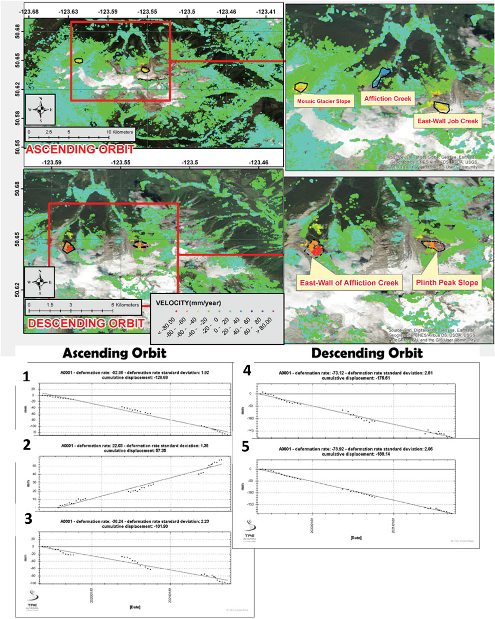
FIGURE 2. SqueeSAR results show deformation rate in mm/year North of the Mount Meager massif; see blue inset in Figure 1B for the location. Note the impact of Line of Sight (LOS) limitation to capture slope deformation for both ascending and descending satellite orbits. The graphs show the temporal deformation rate for 1) East-wall Job Creek. 2) Affliction Creek 3) Mosaic Creek slope in the ascending orbit, and 4) Plinth Peak slope, and 5) East-wall Affliction Creek in the descending orbit.

4 Methodology

The methodology of this paper is twofold (Figure 3). The first part deals with optical image processing and the second part discusses processing Radar satellite images using TRE-Altamira’s SqueeSAR algorithm. The Akh-Defo software developed in this study (Figure 3) is applied to ground and satellite optical imagery. The Akh-Defo version for ground based optical imagery consists of two Jupyter Notebook files which can run on any Integrated Development and Learning Environment (IDE) with the ability to read Jupyter Notebook files (e.g., Visual Studio Code, Jupyter Lab, Jupyter Notebook). The first Jupyter Notebook file includes image-preprocessing (discussed in detail in the Supplementary Material) such as training the Deep-Learning Convolutional Neural Network (DLCNN) model, application of the trained model to classify and differentiate noisy from noise-free images, sorting of images based on hours of each day, and finally image-alignment analysis for quality assessment before image processing for change detection analysis (Figure 3). The second Jupyter Notebook file includes a simple graphical user interface which performs the following steps: 1) image enhancement and definition of the area of interest; 2) static change detection; and 3) dynamic change detection (static and dynamic change detection described below).

FIGURE 3

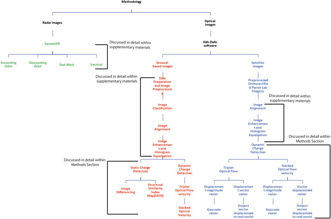
FIGURE 3. Methodology flow chart showing the sequential data processing and analysis in this study.

The Akh-Defo version for satellite optical imagery consists of one Jupyter Notebook file and only processes orthorectified imagery (Figure 3). The software also includes a simple graphical user interface that performs the following steps: 1) image enhancement and definition of the area of interest; 2) static change detection, and 3) dynamic change detection. Unlike the ground-based version, the satellite version enables geocoding and orthorectification of the final products to real-world coordinates for use with any GIS platforms.

4.1 Optical Monitoring

4.1.1 Static Change Detection

Static Change detection includes image differencing such as performing subtraction between two images to identify change of the visual scene or a similarity map to differentiate areas with no change from those with change. We call this static change detection because we can only accurately identify the changes if material (objects) is removed or added within the visual scene between two separate images (Figures 4, 5).

FIGURE 4

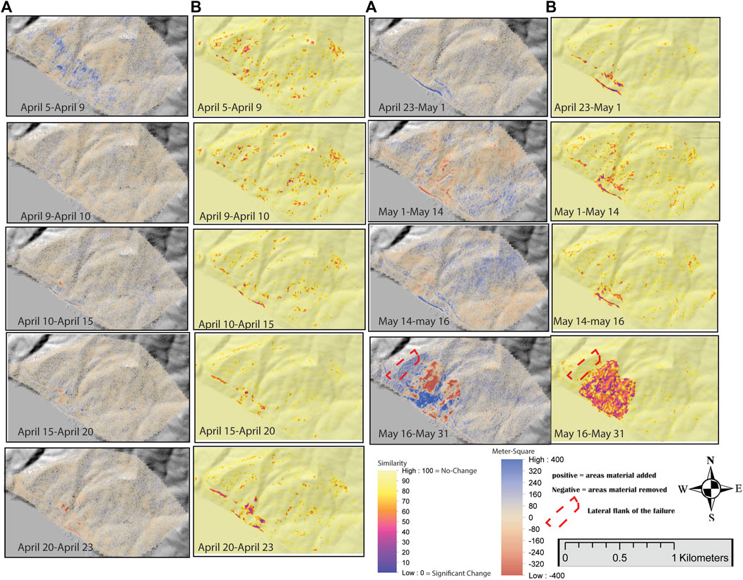
FIGURE 4. Static change detection timestamp results for the Mud Creek landslide. Column (A) shows the image differencing results; negative values indicate areas with material being removed, and positive values indicate area with material being added. (B) shows the Structural Similarity Index Map, similarity map scaled between 0 = no similarity and 100 = strongly similar (no change).

FIGURE 5

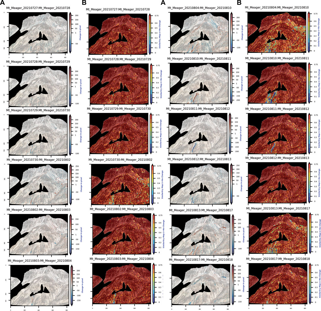
FIGURE 5. Static change detection timestamp results for the Plinth Peak slope. Column (A) shows the image difference results, with negative values indicating areas with material being removed and positive values being added. Column (B) shows the Structural Similarity Index Map, similarity map scaled between 0 = no similarity and 1 = strongly similar (no change).

4.1.1.1 Image Differencing

This technique consists of a pixel-to-pixel value subtraction of an image (Im₁) at specific time, t, for a given date to the same pixel in an image for a different date, Im₂, but at the same time (Figures 4A,5A):

$\mathit{Image} Difference=I{m}_1\text{t}-I{m}_{2}t$

This process is performed sequentially for the temporal images from Plinth Peak. By default, image pixel subtraction produces a significant amount of noise, and the quality of the results depends on the time interval between subsequent images as the pixel intensity changes between images. In this study, the minimum time interval between images is about 24 h, but we compensate for the relatively long-time interval by comparing images at a fixed time in subsequent days.

4.1.1.2 Similarity Indices

The Mean Square error (MSE) and the Structural Similarity Index Mean (SSIM) are two Similarity indices that are frequently used to measure the quality of images (e.g., Palubinskas, 2014; Kim et al., 2020). MSE is considered as a measure of signal fidelity which compares two signals (images) and provides a quantitative score that measures the degree of similarity between them. We assume $\text{x}=\left\{x_i\mathrm{\mid }i=\mathrm{1,2},\cdots ,N\right\}$ and $\text{y}=\left\{y_i\mathrm{\mid }i=\mathrm{1,2},\cdots ,N\right\}$ in which N denotes the number of signal samples (i.e., the number of pixels in an image) such that $x_i$ and $y_i$ are values of pixels at locations x and y. Therefore, MSE can be calculated as follows (Wang and Bovik, 2009, and references therein):

$\text{MSE}\left(x\mathrm{\mid y}\right)=\frac{1}{N}{\displaystyle \sum _{i=1}^N{\left(x_i-y_i\right)}^2}.$

The SSIM technique is based on the human visual system which is particularly powerful in extracting structural information within visual scenes. Hence, to measure similarity, the preservation of signal (image) structure is essential, and it helps to measure the structural distortion (here the distortion related to deformation of the slope). Therefore, SSIM helps to distinguish between structural and nonstructural distortions. Nonstructural distortions include those from the ambient natural environment and instrumental conditions during image acquisition such as 1) Change of luminance or brightness, 2) Change of contrast, 3) Gamma distortion, and 4) Spatial shift of pixels (Palubinskas, 2014; Kim et al., 2020). The structural distortions caused by camera lens and camera mount vibration have been corrected at the image alignment stage (Figure 3); images were only left with distortions related to change in the visual scene.

The SSIM measures similarities of images based on the combination of three independent elements, i.e., the brightness values, the contrast values, and the structure of the visual image scene. Assuming that x and y are the locations of two areas within two images of the same size, the similarity of brightness value becomes l(x,y), the similarity of contrast is c(x,y), and the similarity of the area structures is s(x,y) (Palubinskas, 2014; Kim et al., 2020):

$\begin{array}{c}SSIM\left(\mathrm{x},\text{y}\right)=l\left(\mathrm{x},\text{y}\right)\cdot c\left(\mathrm{x},\text{y}\right)\cdot s\left(\mathrm{x},\text{y}\right)=\left(\frac{2{\mu }_x{\mu }_y+C_1}{{\mu }_x^2+{\mu }_y^2+C_1}\right)\\ \cdot \left(\frac{2{\sigma }_x{\sigma }_y+C_2}{{\sigma }_x^2+{\sigma }_y^2+C_2}\right)\cdot \left(\frac{{\sigma }_{xy}+C_3}{{\sigma }_x{\sigma }_y+C_3}\right)\end{array}$

where ${\mu }_x$ and ${\mu }_y$ are local sample means of x and y areas, respectively. ${\sigma }_x$ and ${\sigma }_y$ are local standard deviations of x and y areas; ${\sigma }_{xy}$ allocates the sample cross-correlation of x and y after removing the means of x and y areas. To avoid numerical instability in calculating sample means, variances and correlations, small positive constants $C_1, C_2$, and $C_3$ were introduced. The SSIM map is produced by computing a sliding window moving pixel-by-pixel across the entire image (Palubinskas, 2014; Kim et al., 2020). A single SSIM score for the whole image is then calculated by averaging the SSIM values across the entire image (Figures 4B,5B).

4.1.2 Dynamic Change Detection

Dynamic Change detection involves calculating optical flow velocity between triplets of images. The temporal period between each image can be anywhere from intervals of 1 day to several days but the images must be taken at the same time of day in order to minimize the effects of ambient change (e.g., shadows). Subsequently, we can calculate temporal and dynamic change detection from a stack of calculated triplets. We call this dynamic change detection because we can identify the change before (pre-cursor of rockfall and landslide), during (e.g., tracing rockfall and landslide flow path) and after (post-failure) material being removed or added within the scene between a number of subsequent images (Figures 6C–F, 7, 8).

FIGURE 6

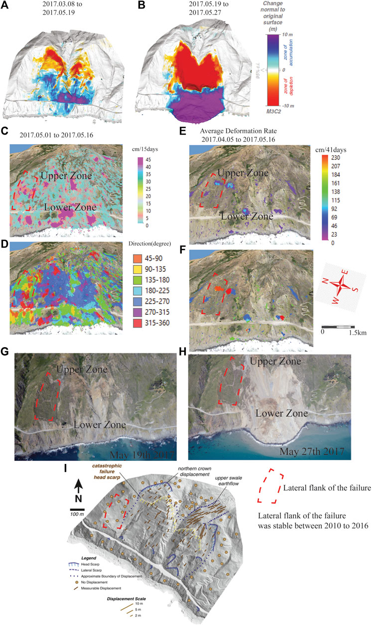
FIGURE 6. Mud Creek landslide precursor changes. (A) Elevation change calculated from SfM digital surface model between March 8 and May 19, 2017 (1 day before failure). (B) Elevation change before and after the catastrophic failure. (C) Dynamic change detection showing horizontal displacement rates in cm per day from May 1 to May 16, 2017 (4 days before failure). (D) Displacement vector r (direction) for panel (C). (E) Average horizontal displacement rate in cm for the 41 days calculated from stacked triplets between April 5 and May 16, 2017 (4 days before the failure). (F) Displacement vector (direction) for panel (E). (G) Oblique Unmanned Aerial Vehicle (UAV) photograph taken 1 day before the May 20, 2017, failure. (H) Oblique UAV photograph taken 7 days after the May 20, 2017, failure. UAV photographs from Warrick et al. (2019). (I) Horizontal displacement map of the Mud Creek site between 2010 and 2016. Locations of observed and mapped head and lateral scarps(blue lines). The head scarp of the May 20, 2017, failure is shown for comparative purposes (yellow line). The approximate boundaries between no displacement and measurable displacement are shown with dashed lines. Shaded relief base-layer map is the May 2016 Lidar (after Warrick et al., 2019).

FIGURE 7

FIGURE 7. Timestamp (number of days before the failure) horizontal displacement rate (cm per days) before the May 20, 2017, landslide. Note the location of the failure surface before and after the landslide.

FIGURE 8

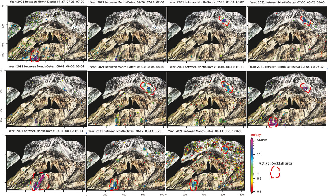
FIGURE 8. Example of dynamic change detection at 2 p.m. daily for the Plinth Peak slope. Refer to the GitHub repository for temporal dynamic change detection results at 11 a.m., 12 p.m., and 1 p.m.

4.1.2.1 Optical Flow Velocity

Optical flow is represented as the apparent motion of objects and surfaces between two different timeframes caused by relative motion between the observer (camera) and the scene (e.g., objects, surfaces, and edges) (O’Donovan, 2005; Zach et al., 2007; Wedel et al., 2009; Hermle et al., 2022). The most important assumption in optical flow velocity calculations is constancy in image brightness. This assumption requires that for a short time interval, t₁ to t₂, an object may change position, while the reflectivity and illumination will remain constant.

Here we process images using an interval of 24 h to a few days, however, it is more difficult to fulfill the assumption of brightness constancy without proper image preprocessing and appropriate image selection for processing. Longer time intervals were compensated by processing images at a fixed time as it helps to remove impact of the angular change in Sun illumination (Figures 7, 8). For processing optical satellite images, while repeated image acquisition is not possible at the same exact time for each day, the images acquired are near vertical (i.e., similar Sun illumination) and we used orthorectified images that have been pre-processed and corrected for atmospheric and geometric noise.

The optical flow equation includes:

$I\left(x+\text{Δ}x,y+\text{Δ}y,t+\text{Δ}t\right)=I\left(x,y,t\right)$

where I(x, y, t) is the intensity of the image at position (x, y) for time t and the change in position is indicated by $\text{Δ}x and \text{Δ}y$ at change of time $\text{Δ}t$. After applying a Taylor series expansion to the left hand side of the equation, it can be rewritten as follows (O’Donovan, 2005; Zach et al., 2007; Wedel et al., 2009; Hermle et al., 2022):

$I\left(x+\text{Δ}x,y+\text{Δ}y,t+\text{Δ}t\right)=I\left(x,y,t\right)+\frac{\partial I}{\partial x}\text{Δ}x+\frac{\partial I}{\partial x}\text{Δ}y+\frac{\partial I}{\partial t}\text{Δ}t$

By solving the above equation, we obtain the optical flow constraint equation:

$\nabla I\cdot \text{v}+I_t=0$

where $\nabla I$ is the spatial intensity gradient (I_x, I_y), v = (u, v) is the flow vector for $\text{Δ}x \text{and} \text{Δ}y$ and $I_t$ is gradient through time.

Additionally, to better compensate for the image time interval, we calculate the optical flow for triplets of images (frames) instead of pairs of images. The sequence of image triplets is chosen in order to provide overlap among subsequent processed triplet datasets (Figure 7). For instance, (image_n, image_n+1, and image_n, image_n+2) forms the first triplet set; the second triplet set is equal to (image_n+1, image_n+2, and image_n+1, image_n+3) and so on for the rest of the image sequences. The calculated optical flow movements are then stacked for the horizontal $\frac{\text{Δ}x}{\text{Δ}t}$, and vertical $\frac{\text{Δ}y}{\text{Δ}t}$, obtained from each set of processed triplets. The stacking process allows us to calculate more accurate optical flow motion because it uses larger number of images and averages the results of the calculated triplet optical velocities. Additionally, it provides measurements over a longer time interval of months to even multiple years depending on the number of available processed triplets and the time-window of the triplet datasets (Figures 6C–F, 7, 8).

4.1.3 Radar Monitoring

4.1.3.1 Synthetic Aperture Radar

Synthetic Aperture Radar (SAR) satellites acquire images of the Earth’s surface by emitting electromagnetic waves and analyzing the reflected signal. As SAR satellites are continuously orbiting the globe, a stack of SAR images can be collected for the same area over time to extract information about changes of the Earth’s surface. Each SAR acquisition contains two fundamental properties: amplitude and phase. The amplitude is related to the energy of the backscattered signal and is used in Speckle/Pixel Tracking applications and change detection mapping. Phase is related to the sensor-to-target distance, and it is this which is used in interferometric applications.

4.1.3.2 InSAR

Interferometric Synthetic Aperture Radar (InSAR), also referred to as Interferometric SAR, is the measurement of signal phase change or interference over time. When a point on the ground moves, the distance between the sensor and the ground target changes affecting the phase value recorded by the SAR sensor. Figure 2 shows the relationship between ground movement and the corresponding shift in signal phase between two SAR signals acquired over the same area. This relationship is expressed as:

$\text{Δ}\phi =\frac{4\pi }{\lambda }\text{Δ}R$

where $\text{Δ}\phi$ is the change in signal phase, λ is the wavelength and ΔR is the displacement. Consequently, any displacement of a radar target along the satellite Line of Sight (LOS) creates a phase shift in the radar signal that can be detected by comparing the phase values of two SAR images acquired at different times. Due to the acquisition geometry, any phase variation is detected along the satellite LOS. In general, due to the known parameters of SAR satellite orbits and acquisition geometry (approximate North-South orbital direction and side and tilted view), InSAR can detect motion components predominantly in E-W and vertical directions. In contrast, the sensitivity to N-S motion is minimal, even in the presence of strong movement. The comparison of the phase of two SAR images can only be used when the normal baseline (i.e., distance between the satellite tracks during the first and second acquisitions) is no more than the so-called “critical baseline”, a parameter depending on the SAR sensor in use.

4.1.3.3 SqueeSAR

SqueeSAR™ is the proprietary multi-interferogram technique developed by TRE Altamira which provides high precision measurements of ground displacement by processing multi-temporal SAR images acquired over the same area. SqueeSAR™ typically needs a dataset of at least 15–20 SAR images to be applied, acquired over the same area with the same acquisition mode and geometry. By statistically exploiting the image stack, SqueeSAR™ singles out measurement points (MP) on the ground that display stable amplitude and coherent phase throughout every image of the dataset (Ferretti et al., 2011). The MPs belong to two different families: 1) Permanent Scatterers (PS) point-wise radar targets characterized by high stable radar signal return (e.g., buildings, rocky outcrops, linear structures, etc.) and 2) Distributed Scatterers (DS) such as areas of ground exhibiting a lower but homogenous radar signal return (e.g., uncultivated land, debris, deserted areas, etc.). The density and distribution of the MP is related to the resolution of the SAR images used and the local surface characteristics and topography.

In general, the MP density increases with the satellite resolution and the presence of man-made structures and decreases with the presence of vegetation. The highest density is reached over urban and bare areas, while it is lower over areas heavily vegetated areas, affected by strong reflectivity changes with time (Figure 2 and Supplementary Table S2 in supplementary material) or where the satellite visibility is limited. No measurement points are identifiable over water. For each MP identified, SqueeSAR™ provides the following basic information: 1) The ground target’s position and elevation; 2) Annual average displacement rate measured along the LOS, expressed in mm/year; calculated over the observation period and related to the reference point; 3) Displacement time series (TS) representing the evolution of the MP’s displacement for each acquisition date, expressed in millimeters, and measured in the LOS direction.

When considering the Distributed Scatterer family of MPs, the information provided by SqueeSAR™ does not refer to a single target, but rather to the effective area associated to each DS. SqueeSAR™ does not provide the exact shape of the DS area only its dimension. As for any other InSAR analysis, all displacement measurements are carried out along the sensor’s LOS to target direction. SqueeSAR™ measures the projection of real movement along the LOS and provides 1D measurements. Displacement measurements provided by SqueeSAR™ are differential in space and time. They are spatially related to a reference point and temporally to the date of the first available satellite acquisition. The reference point is assumed to be motionless and selected for its radar properties and motion behavior. This corresponds to a radar target with low phase noise in all the scenes of the imagery, not affected by displacement rate variations (non-linear movement or cyclical deformations) in the covered period. As such, the reference point can still be affected by a linear movement related to regional deformation phenomena. Any regional component can be identified via an independent check with other surface monitoring techniques, such as a GPS network. The selection of the reference point is imagery dependent: if the imagery changes (e.g., number of scenes in the stack or time span), the MP selected as the reference point can consequently change.

5 Results

5.1 Plinth Peak, Mount Meager, Canada

Results from the high temporal and spatial resolution InSAR data (summer 2019–2021), processed with SqueeSAR, identified at least five highly unstable regions on the North flank of the Mount Meager massif. These regions were observed with the ascending SAR satellite geometry and show annual average deformation rates of 5.2, 2.2 and 3.8 cm for Mosaic Glacier slope, Affliction Creek, and East-Wall Job Creek, respectively (Figure 2). The unstable regions observed via descending SAR satellite geometry show annual average deformation rates of 7.8 and 7.3 cm for East-Wall Affliction Creek and Plinth Peak slopes, respectively (Figure 2).

We processed both ground-based optical images and orthorectified satellite images for Plinth Peak within the same time-window. Ground-based imagery processed with the Akh-Defo dynamic change detection technique measured monthly deformation rates on Plinth Peak from 27 July to 18 August 2021, of between 7 and 27 mm (Table 1; Figure 9). Low velocity rockfall (less than 600 mm/day) (Figure 8) but frequent (Figure 10) were observed during the four different daily time periods between 27 July and 18 August 2021. The total detected rockfalls at each time window are as follows: 15 events at 11 a.m., 15 events at 12 p.m., seven events at 1 p.m., and 10 events at 2 p.m. (Figure 8). A small landslide was identified on 11 August 2021, with an area of more than 3,500 m² (Figure 9). By contrast, PlanetLab orthorectified imagery processed with the Akh-Defo dynamic change detection was unable to quantify the rockfall activity on Plinth Peak. This is particularly related to the geometry of the camera viewing angle.

TABLE 1

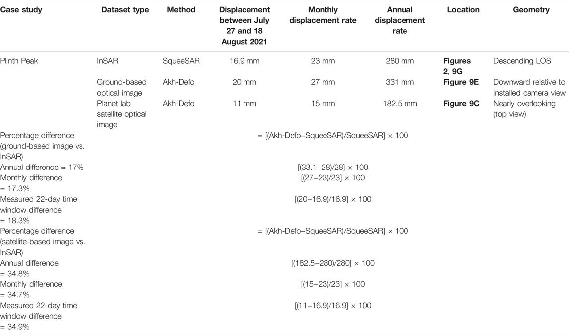
TABLE 1. Semi-quantitative comparison of measured land displacement obtained from Akh-Defo software for Plinth Peak with three independent sources: radar images, ground-based optical images, and orthorectified optical satellite images.

FIGURE 9

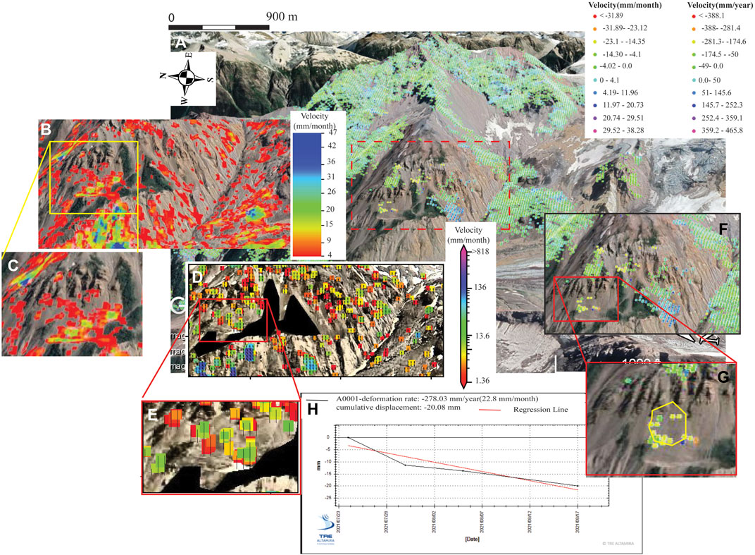
FIGURE 9. Comparison between Plinth Peak slope displacement from InSAR and average displacement rate calculated from stacked optical velocity triplets for the period from July 27 to 18 August 2021. (A) Sliced-time window of SqueeSAR results between July 24 and 17 August 2021; red dashed rectangle is zoom in location for panels (B,D,F). (B,C) are close ins of stacked optical flow velocity calculated from orthorectified optical satellite images. (D,E) are close ins of stacked optical flow velocity calculated from ground-based optical images. (F,G) are close ins of processed time-series radar images using SqueeSAR. (H) InSAR displacement timeseries for the yellow polygon in (G) See Figure 1 to locate the extent of Figure 9. The colour bar for panels (D,E) represented as logarithmic scale.

FIGURE 10

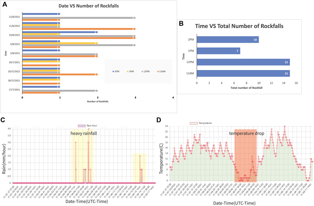
FIGURE 10. (A) Number of observed rockfalls during four daily time periods (11 a.m., 12 p.m., 1 p.m., and 2 p.m.) between July 27 and 18 August 2021. (B) Total number of rockfalls during these time periods. (C) Hourly rainfall data between July 27 and 18 August 2021. (D) Hourly temperature data between July 27 and 18 August 2021.

The land displacement results are validated from the calculated displacement rates from SqueeSAR for the equivalent period (Table 1) and at a location where we have active displacement data available from both techniques. The validation includes normalization of SqueeSAR annual displacement rates to match displacement rates for the same period of Akh-Defo dataset of 22 days (Table 1). At the location shown in Figure 9E, for the 22 days between 27 July and 18 August 2021, Akh-Defo stacked processing obtained a total displacement of 20 mm (equivalent 27 mm per month) (downward relative to the camera view; see Figure 1 for the camera orientation and location). Comparatively, at the same site and time window (Figure 9G), the SqueeSAR deformation results obtained a ground displacement of 16.9 mm (22.5 mm per month), along SAR satellite LOS (Descending Orbit). Additionally, the PlanetLab.

Our ground-based imagery results show that the Plinth Peak slope is subject to active and frequent rockfalls albeit with slow slope displacement and that the rockfalls are mainly concentrated along very-steep channels within the slope (Figure 10 rockfall frequency and Figure 11 for sources of rockfalls). Rockfall trajectories were validated from the animated image time-lapse (see the online GitHub in the gif_dir folder dataset).

FIGURE 11

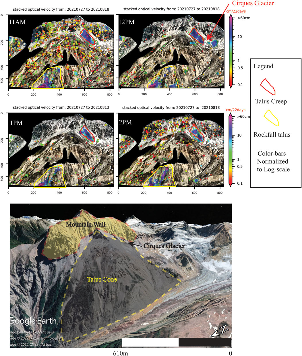
FIGURE 11. Average displacement rate and average magnitude velocity of rockfalls calculated from a stack of processed image triplets for four different times of the day for the Plinth Peak slope. Note that the rockfall region areas show average magnitude velocity of rockfalls ranging between 20 and 60 cm.

The Akh-Defo static change detection (using Image Differencing and Structural Similarity Index Map) was effective in identifying one small landslide (rockslide) on the Plinth Peak slope, approximately 30-m-wide and 120-m-long (at least 3,600 m²) between 10 and 11 August 2021, although with different sensitivities (Figure 12). For the same landslide, the SSIM visually produced clearer results compared with those using Image Differencing (Figure 12). In fact, we also captured a precursor of this event using dynamic change detection 7 days before failure where the total displacement ranged from 1 to 10 cm from 3 to 10 August 2021 (Figure 12G). Additionally, we reconstructed the rockslide trajectory and velocity of the rockslide at >60 cm/day between 10 and 12 August 2021 (Figure 12H).

FIGURE 12

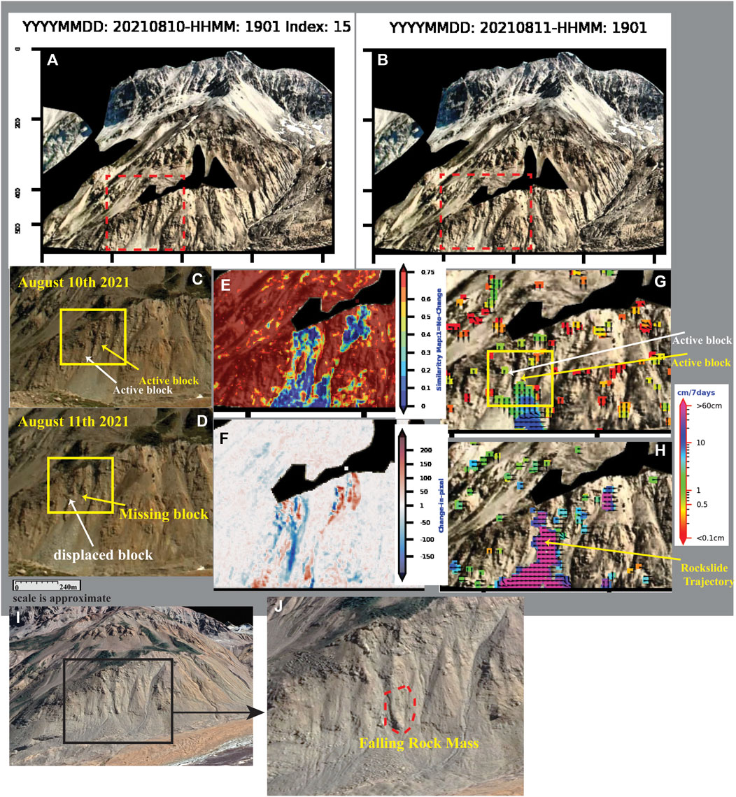
FIGURE 12. Small landslide identification with Akh-Defo using combined static and dynamic change detection methods for the Plinth Peak slope. (A) Image taken on 10 August 2021, at 11 a.m. (B) Image taken on 11 August 2021, at 11 a.m. (C) Zoomed window of panel (A) focused on the unstable region before the rockslide failure occurred on 10 August 2021. (D) Zoomed window of panel (B) focused on the unstable region after the rockslide failure occurred on 11 August 2021. (E) Results of the structural similarity index map. Note the rockslide and change identification obtained from structural similarity map compared to image differencing. (F) Results of image differencing showing areas of change and rockslide events. (G) Displacement rate for the Plinth Peak slope calculated from triplets of images 7 days before the 11 August 2021, rockslide event. (H) Reconstructed trajectory path of the rockslide. The colour bar for panels (G,H) is log scale. (I) High resolution Google Earth imagery showing the least stable part of Plinth Peak slope. (J) Zoomed window of panel (I) show approximate size and location of the failing rock mass on 11 August 2021.

The mechanism of the rockfalls and the rockslide can be further quantified based on the morphology of the Plinth Peak slope. The slope is composed of a large talus cone (Rapp and Fairbridge, 1997) formed due to the accumulation of rock-debris at its base (Figure 11). The bedrock of the slope is composed of rhyodacite lavas which may have facilitated relatively uniform weathering across the West part of the Plinth Peak resulting in a single talus slope rather than a series of cones. According to Rapp and Fairbridge (1997), rates of creep movement in active talus cones can be ∼10 cm/year on the upper part of the cone decreasing to zero towards the base. These rates are similar to the SqueeSAR displacement rates for Plinth Peak of 7.3 cm/year (Figure 2).

The rockfalls detected by Akh-Defo on the Plinth Peak slope can be categorized into two types of talus deposits, rockfall talus and talus creep (Rapp and Fairbridge, 1997). Rockfall talus related to individual block failing, such as the 11 August rockslide, are characterized by shattering, rolling, and bouncing caused by freeze-thaw, and heavy rain (Figures 10C,D, 11, 12). One week before the 11 August 2021, rockslide, the camera weather station recorded a sharp drop in temperature as well as heavy rainfall (Figure 10).

Although, at this time there is no published information regarding the structural and kinematic behavior of the Plinth Peak slope, we performed a preliminary assessment in order to map linear features from the Lidar-based hillshade map. The Plinth Peak slope encompasses at least three sets of lineaments, striking NW-SE, ESE-WNW, and NNE-SSW. Our results show that most of the rockfalls and slope deformation occur within and along the trends of mapped lineaments (Figure 13) with rockfalls particularly concentrated along the NNE-SSW striking lineaments.

FIGURE 13

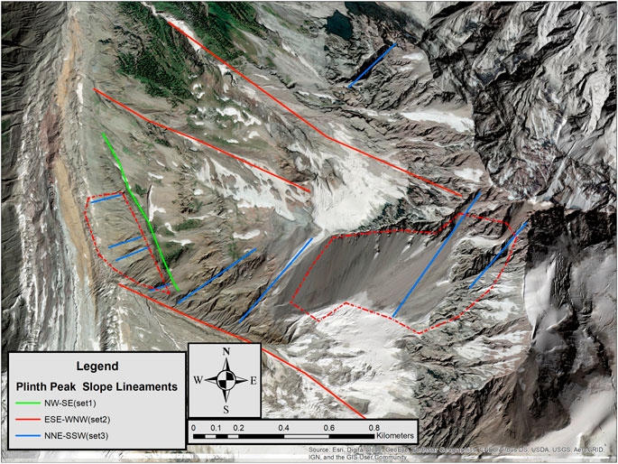
FIGURE 13. High resolution ESRI satellite image overlayed on top of the lidar-based hillshade map; shown are three sets of lineaments that most likely structurally control the Plinth Peak slope deformation. The dashed red polygon represents areas of frequent rockfall.

5.2 Mud Creek Landslide, California

Akh-Defo processing of orthorectified PlanetScope satellite imagery identified displacement between 50 and 300 cm (Figures 6, 7), 41 days prior to the 20 May 2017, Mud Creek landslide. The timestamp-sequential displacement (Figure 7) and average displacement (Figure 6) show two main unstable zones. The upper zone (referred to as the depletion zone by Warrick et al., 2019) showed a maximum of 100 cm displacement on 10 April 2017, 40 days before the catastrophic landslide failure. In comparison, the lower zone (referred to as the accumulation zone by Warrick et al., 2019) showed displacement rates of as little as 60–80 cm for the same time period 40 days before the failure (Figure 6).

This failure event was followed by accelerating displacement in the lower zone from 80 cm to more than 300 cm at 35 and 6 days, respectively, before the catastrophic failure (Figure 7). Four days before the event, both the upper and lower zones became extremely unstable and showed displacement of more than 300 cm. The above pattern of accelerating displacement in the lower zone at days 35 to 6, preceding the upper zone, might have facilitated the occurrence of the catastrophic failure. This would kinematically validate the loss of slope piedmont support for material from the upper slope zone. Warrick et al. (2019) show that although the lateral flank of the failure moved significantly during the failure, it did not fail completely (Figures 6G,H). We were able to measure average displacement of 80 cm for the lateral flank 41 days before the catastrophic failure (Figures 6E,F; Table 2) which increased to a few meters between May 1 and 16, 2017, just 4 days before the catastrophic failure (Figure 7).

TABLE 2

TABLE 2. Average displacement from two independent datasets prior to the 20 May 2017, Mud Creek landslide.

Although there is limited data and information available regarding the cause of the Mud Creek 2017 landslide, according to Handwerger et al. (2019), the region underwent a 5-year drought before 2017 and the failure occurred following a period of persistent rainfall lasting several days. Simple 1D hydrological modelling suggests that significant increases in pore-fluid pressure led to rapid destabilization of the slope resulting in the catastrophic Mud Creek landslide.

6 Discussion

Aside from data preprocessing, the main task of Akh-Defo is to perform static and dynamic change detection. Dynamic change detection is a powerful method for slope deformation monitoring as it provides pre-failure warning signals—for example, 7 days before the 11 August 2021, rockslide on Plinth Peak, the software measured >2 cm of slope movement at the rockslide source area (Figures 12G,H); additionally, 41 days before the 20 May 2017, Mud Creek landslide, the Akh-Defo software measured more than 50 cm of slope movement (Figures 6, 7).

Static change detection consists of image difference maps through subtraction of subsequent images and similarity maps through measuring image similarities based on the combination of three independent elements: 1) brightness values, 2) contrast values, and 3) structure of the visual image scene. Unlike similarity maps, image differencing solely relies on pixel intensity change between subsequent images; hence, it is sensitive to light conditions and produces relatively more noise (Figure 14). For instance, changes in solar elevation angle produce different Sun illumination patterns and different shade patterns on ground surfaces at different hours of the day. We minimized light condition variability related to daily change of Sun elevation angle and Sun azimuth at different hours of the day by processing images acquired at the same time of the day (Figure 14).

FIGURE 14

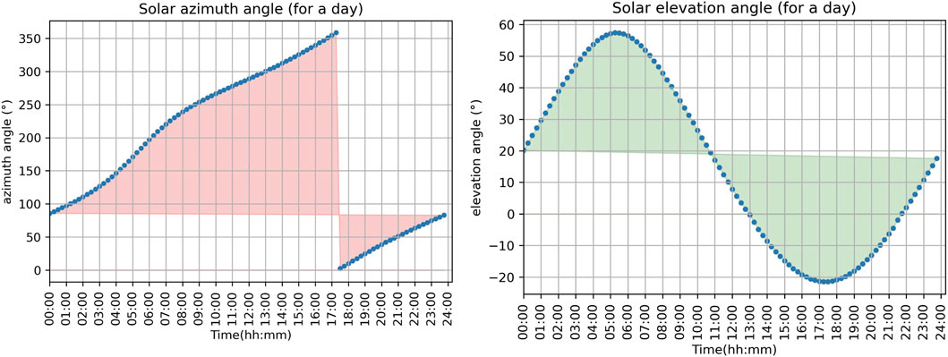
FIGURE 14. Solar elevation and azimuth change for the Mount Meager area during August 2021. Note the change of solar elevation angle relative to change of solar azimuth angle during the day. Data from (https://keisan.casio.com/exec/system/1224682277).

The Dynamic Change-Detection approach can detect slow (sub-cm) and fast (more than a few metres) slope movement. The user needs to apply other complementary techniques to differentiate the source of calculated displacement such as rockfall, rockslide or slow slope deformation. In this study we used a number of methods to distinguish and interpret the source of slow and fast displacement rates including SqueeSAR, Static Change-Detection and visual observation of the time-lapse images. SqueeSAR (InSAR) is a valuable independent method to validate slow slope displacement (Table 1; Figure 9). Static change detection and visual observation of the image time-lapse both are important to quantify fast slope movement such as rockfalls and rockslides (Figures 10, 12).

Through installation of a low-cost fixed camera and telemetry system, we were able to collect more frequent images (daily to hourly) of the Plinth Peak slope compared to exclusively relying on InSAR (Figures 9G,E). Statistical comparison between SqueeSAR results and Akh-Defo shows less than 20% difference in displacement rate from Akh-Defo relative to InSAR (Table 1). SqueeSAR processes radar images and relies on the change of distance between the SAR satellite and the target on the ground. SqueeSAR can processes data collected at all times and under various weather conditions such as cloud, fog, and rain. However, SqueeSAR cannot calculate sufficient measurement points in very steep slopes or if the target invisible to the LOS.

Alternatively, Akh-Defo processes optical images and relies on the change of the intensity pattern within the optical image but is restricted to only data collected during the daytime and under clear weather conditions. In this study, the Akh-Defo software was applied to the Planet Labs pre-processed orthorectified optical images to measure the Plinth Peak slope as well as the pre–Mud Creek landslide movements. The calculated land movement from orthorectified satellite optical images are more accurate and easier to project to the real-world trajectories relative to the ground-based optical images, mainly due to the geometric characteristics of the satellite images relative to the ground images. For instance, in the case of orthorectified satellite images, the pre-processed optical images have already been corrected (using digital elevation models) for external image distortion caused by the difference in depth of objects within the image scene (i.e., any distortions caused by topography have been corrected).

Akh-Defo uses optical flow algorithms to calculate slope movement. The measurement accuracy depends on the data-collection system such as resolution of the raw image, weather conditions during capturing the image, stability of the camera system (in case of ground-based images) and even time of the day the subsequent images were taken. In our methodology, we were careful to select images for processing to obtain acceptable results for validation with other independent systems such as SqueeSAR (Plinth Peak case study) and Lidar DEM change detection (Mud Creek case study). For instance, we only processed images taken during clear weather conditions (no fog, snow, or rain), we performed image alignment to compensate for the stability of the ground camera system (see Supplementary Material for image alignment process) and we only processed images taken at fixed hour of subsequent days. In addition to careful selection of images and image pre-processing steps such as image alignment and image enhancement, we also integrated similarity thresholds (comparable to InSAR coherence thresholds). The advantage of using this parameter is that it enables calculation of displacement velocity only for pixels with known stable texture and light condition (Figures 15B,D).

FIGURE 15

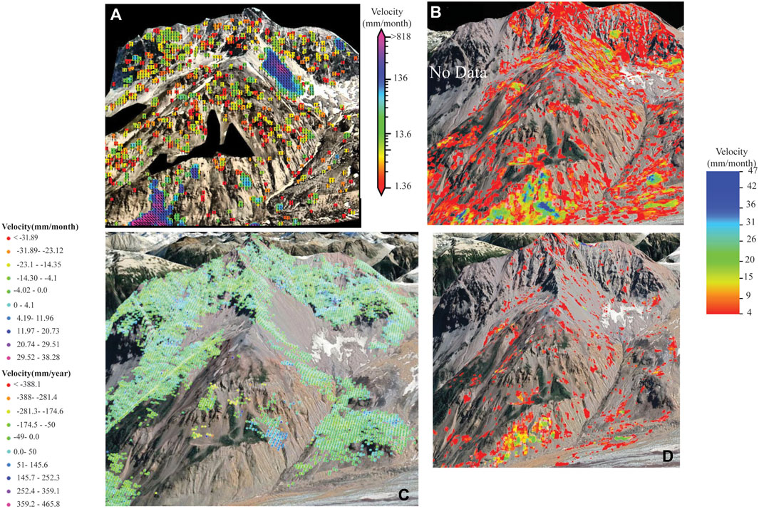
FIGURE 15. Deformation rates in millimeter per month for Plinth Peak slope. (A) Deformation rate calculated from ground-based optical images from July 27 to 18 August 2021; note, the colour-bar is shown as a logarithmic scale, deformation rates larger than 20 mm represents traces of slow but continuous rockfalls within the processed time window period. (B) Deformation rate calculated from orthorectified optical satellite images from July 28 to 13 August 2021, deformation map processed with similarity threshold equal to 0.75. (C) Deformation rate calculated from radar images for summer 2019, 2020, and 2021 using TRE-ALTAMIRA SqueeSAR Software. SqueeSAR by default calculate annual deformation rate, we rescaled to a monthly deformation rate. (D) Deformation rate calculated from orthorectified optical satellite images from July 28 to 13 August 2021, deformation map processed with similarity threshold equal to 0.2.

Current limitations of the Akh-Defo software include the inability to accurately identify the displacement vector field for the calculated displacement from the ground-based images processed for the Plinth Peak slope. This limitation is inherent to all computer vision optical flow codes and its known as the Aperture problem (Xue et al., 2015). The significance of the aperture problem depends on the size of the object of interest; for instance, if the object of interest is larger than what can be seen through the camera scene view (such as the Plinth Peak slope), we can only estimate an approximate vector field for objects within the slope. In other words, while we cannot identify the movement of the entire slope relative to Mount Meager itself, we can calculate the displacement rate and vector of smaller landslides and rockfalls withing the field of view of our installed camera.

Another limitation is that the optical flow algorithm can only measure horizontal displacement in a 2-dimensional image space such as (left, right, top, and bottom). This becomes more challenging in the case of ground-based optical image processing to translate the calculated displacement magnitude vector into a real-world vector motion. In contrast, for optical satellite images the solution becomes relatively more practical by processing orthorectified optical images (Figure 3); we can then reproject the calculated velocity magnitude and vector back to the real-world projection using available digital elevation models (Figures 5C,D).

Our results show that ground-based optical images are more suitable to monitor rockfalls compared to orthorectified satellite optical images. This is mainly related to the different angles of view as the orthorectified satellite images are acquired at nearly nadir while ground-based optical images have a nearly horizontal view (Figure 15).

7 Conclusion

In this study, we developed software to process ground-based optical images and orthorectified Planet Lab satellite optical images. The ground-based optical images were used to test the capability of the developed software to complement InSAR LOS limitations for the steep slopes of Plinth Peak. Our ground-based camera analysis, using stacks of optical images from 27 July to 18 August 2021, gives comparable and complementary results (less than 20% difference; see Table 1) for the same time-period with SqueeSAR. In addition to defining deformation rates, we were able to characterize velocity of rockfall trajectories spatially within the slope itself. Additionally, we used two techniques, Image Differencing and Structural Similarity Index (SSIM), to identify areas of significant slope change such as landslide areas. Results from ground-based camera monitoring detected movements of the slope and defined areas of highest rockfall on the western flank of Plinth Peak. Our results show that ground-based optical images are more suitable to monitor rockfalls compared to orthorectified satellite optical images.

We also tested the Akh-Defo program to calculate the pre-failure movement 41 days before the catastrophic 20 May 2017 Mud Creek Landslide from the orthorectified Planet Lab satellite imagery and validated our results with those from Warrick et al. (2019). We calculated timestamp (Figure 7) and average (Figures 6C–G) displacement for the period 40 days before the catastrophic landslide occurred.

In this paper, the following conclusions are presented to enhance cost-effective and near real-time early warning landslide and rockfall monitoring:

1) Radar satellite datasets are a highly effective source to identify unstable areas as a baseline knowledge if followed by less-expensive but continuous ground-based and optical satellite monitoring.

2) Computer vision codes such as optical-flow velocity are highly effective for calculating land deformation semi-quantitively if used with a proper methodological workflow which includes choosing the appropriate type of image dataset and reasonable image pre-processing preparation.

3) Structural similarity maps appear to be more effective in identifying rockfall events and areas of change compared to classic image differencing.

4) The pre-failure Mud Creek displacement results calculated by Akh-Defo software indicate that Akh-Defo program (based on optical flow velocity code) can be used as a first stage preliminary warning system (particularly if run on the Cloud) prior to processing more expensive but more accurate InSAR products such as SqueeSAR.

Data Availability Statement

The datasets presented in this study can be found on the below Online GitHub Repository https://github.com/mahmudsfu/AkhDefo. This repository includes the following materials: A copy of the developed Akh-Defo Python-based software for Ground-based Image processing. A copy of the modified Akh-Defo program to process Planet Labs orthorectified images Ground-based Plinth Peak image dataset evaluated with the Akh-Defo software Mud-Creek Planet Lab orthorectified satellite images evaluated with the modified Akh-Defo software. Plinth Peak Planet Lab orthorectified satellite images evaluated with the modified Akh-Defo software. A step-by-step instruction manual on how to run Akh-Defo software on Jupyter notebook program.

Author Contributions

All authors contributed to writing, processing data and reviewing this manuscript. MM developed the python code and methodology supervised by GW-J and DS. GF and RT processed Radar images using SqueeSAR.

Conflict of Interest

Authors RT and GF are employed by TRE ALTAMIRA, Canada.

The remaining authors declare that the research was conducted in the absence of any commercial or financial relationships that could be construed as a potential conflict of interest.

Publisher’s Note

All claims expressed in this article are solely those of the authors and do not necessarily represent those of their affiliated organizations, or those of the publisher, the editors and the reviewers. Any product that may be evaluated in this article, or claim that may be made by its manufacturer, is not guaranteed or endorsed by the publisher.

Acknowledgments

We wish to thank two reviewers for providing constructive reviews that enhanced the quality of the manuscript. Many thanks to Nupoint Systems Inc. for donating the ground-based camera and weather system and to Weir-Jones Engineering for its installation and repeated maintenance. Thanks also to Energex Renewable Energy and the Meager Creak Development Corporation for technical and logistical support. The Planet Lab company provided access to the satellite imagery via an educational license to SFU. This work was supported by the Canadian Space Agency (CSA), and Mitacs Accelerate and NSERC Discovery grants to GW-J.

Supplementary Material

The Supplementary Material for this article can be found online at: https://www.frontiersin.org/articles/10.3389/feart.2022.909078/full#supplementary-material

References

Amaki, K., Yamaguchi, T., and Harada, H. (2019). “Landslide Occurrence Prediction Using Optical Flow,” in 2019 19th International Conference on Control, Automation and Systems (ICCAS) (Jeju, Korea: IEEE), 1311–1315. doi:10.23919/ICCAS47443.2019.8971698

CrossRef Full Text | Google Scholar

Bouti, A., Mahraz, M. A., Riffi, J., and Tairi, H. (2020). A Robust System for Road Sign Detection and Classification Using LeNet Architecture Based on Convolutional Neural Network. Soft Comput. 24, 6721–6733. doi:10.1007/s00500-019-04307-6

CrossRef Full Text | Google Scholar

Ferretti, A., Fumagalli, A., Novali, F., Prati, C., Rocca, F., and Rucci, A. (2011). A New Algorithm for Processing Interferometric Data-Stacks: SqueeSAR. IEEE Trans. Geosci. Remote Sens. 49, 3460–3470. doi:10.1109/TGRS.2011.2124465

CrossRef Full Text | Google Scholar

Ferretti, A., Monti-guarnieri, A., Prati, C., Rocca, F., and Massonnet, D. (2007). InSAR Principles: Guidelines for SAR Interferometry Processing and Interpretation. Netherlands: ESA Publications. TM-19. ISBN 92-9092-233-8.

Google Scholar

Ferretti, A. (2014). Satellite InSAR Data: Reservoir Monitoring from Space (EET 9). Houten, Netherlands: EAGE. Available at: https://bookshop.eage.org/product/satellite-insar-data-reservoir-monitoring-from-space-eet-9/.

Google Scholar

Foroosh, H., Zerubia, J. B., and Berthod, M. (2002). Extension of Phase Correlation to Subpixel Registration. IEEE Trans. Image Process. 11, 188–200. doi:10.1109/83.988953

PubMed Abstract | CrossRef Full Text | Google Scholar

Friele, P. A., and Clague, J. J. (2004). Large Holocene Landslides from Pylon Peak, Southwestern British Columbia. Can. J. Earth Sci. 41, 165–182. doi:10.1139/e03-089

CrossRef Full Text | Google Scholar

Guthrie, R. H., Friele, P., Allstadt, K., Roberts, N., Evans, S. G., Delaney, K. B., et al. (2012). The 6 August 2010 Mount Meager Rock Slide-Debris Flow, Coast Mountains, British Columbia: Characteristics, Dynamics, and Implications for Hazard and Risk Assessment. Nat. Hazards Earth Syst. Sci. 12, 1277–1294. doi:10.5194/nhess-12-1277-2012

CrossRef Full Text | Google Scholar

Handwerger, A. L., Huang, M.-H., Fielding, E. J., Booth, A. M., and Bürgmann, R. (2019). A Shift from Drought to Extreme Rainfall Drives a Stable Landslide to Catastrophic Failure. Sci. Rep. 9, 1569. doi:10.1038/s41598-018-38300-0

PubMed Abstract | CrossRef Full Text | Google Scholar

Hermle, D., Gaeta, M., Krautblatter, M., Mazzanti, P., and Keuschnig, M. (2022). Performance Testing of Optical Flow Time Series Analyses Based on a Fast, High-Alpine Landslide. Remote Sens. 14, 455. doi:10.3390/rs14030455

CrossRef Full Text | Google Scholar

Hetherington, R. (2014). Slope Stability Analysis of Mount Meager, South-Western British Columbia (Michigan Technological University), 68. MSc Thesis. Available at: http://digitalcommons.mtu.edu/etds/764.

Holst, C., Janßen, J., Schmitz, B., Blome, M., Dercks, M., Schoch-Baumann, A., et al. (2021). Increasing Spatio-Temporal Resolution for Monitoring Alpine Solifluction Using Terrestrial Laser Scanners and 3d Vector Fields. Remote Sens. 13, 1192. doi:10.3390/rs13061192

CrossRef Full Text | Google Scholar

Javier, S., Meinhardt-llopis, E., and Facciolo, G. (2013). TV-L1 Optical Flow Estimation. Image Process. Line 3, 137–150. doi:10.5201/ipol.2013.26

CrossRef Full Text | Google Scholar

Khan, M. W., Dunning, S., Bainbridge, R., Martin, J., Diaz-Moreno, A., Torun, H., et al. (2021). Low-cost Automatic Slope Monitoring Using Vector Tracking Analyses on Live-Streamed Time-Lapse Imagery. Remote Sens. 13, 893. doi:10.3390/rs13050893

CrossRef Full Text | Google Scholar

Kim, D., Balasubramaniam, A. S., Gratchev, I., Kim, S. R., and Chang, S. H. (2020). “Application of Image Quality Assessment for Rockfall Investigation,” in 16th Asian Regional Conference on Soil Mechanics and Geotechnical Engineering (Taipei, Taiwan: ARC). Available at: http://seags.ait.asia/16arc-proceedings/16arc-proceedings/.

Google Scholar

Kromer, R. A., Abellán, A., Hutchinson, D. J., Lato, M., Chanut, M.-A., Dubois, L., et al. (2017). Automated Terrestrial Laser Scanning with Near-Real-Time Change Detection - Monitoring of the Séchilienne Landslide. Earth Surf. Dynam. 5, 293–310. doi:10.5194/esurf-5-293-2017

CrossRef Full Text | Google Scholar

Lin, Z., Kaneda, H., Mukoyama, S., Asada, N., and Chiba, T. (2013). Detection of Subtle Tectonic-Geomorphic Features in Densely Forested Mountains by Very High-Resolution Airborne LiDAR Survey. Geomorphology 182, 104–115. doi:10.1016/j.geomorph.2012.11.001

CrossRef Full Text | Google Scholar

Mokievsky-Zubok, O. (1977). Glacier-caused Slide Near Pylon Peak, British Columbia. Can. J. Earth Sci. 14, 2657–2662. doi:10.1139/e77-230

CrossRef Full Text | Google Scholar

O’Donovan, P. (2005). Optical Flow: Techniques and Applications. Available at: http://www.dgp.toronto.edu/∼donovan/stabilization/opticalflow.pdf.

Google Scholar

Palubinskas, G. (2014). “Mystery behind Similarity Measures Mse and SSIM,” in 2014 IEEE International Conference on Image Processing (ICIP) (Wessling, Germany: IEEE), 575–579. doi:10.1109/ICIP.2014.7025115

CrossRef Full Text | Google Scholar

Planet Team (2017). “Planet Application Program Interface,” in Space for Life on Earth (Fort Mill, SC: Planet Publications.

Google Scholar

Rapp, A., and Fairbridge, R. W. (1997). “Talus Fan or Cone; Scree and Cliff Debris,” in Geomorphology (Dordrecht: Kluwer Academic Publishers), 1106–1109. doi:10.1007/3-540-31060-6_367

CrossRef Full Text | Google Scholar

Read, P. (1990). Mt Meager Complex, Garibaldi Belt, Southwestern BC. Geoscience 17, 167–170.

Google Scholar

Roberti, G., Friele, P., van Wyk de Vries, B., Ward, B., Clague, J. J., Perotti, L., et al. (2017). Rheological Evolution of the Mount Meager 2010 Debris Avalanche, Southwestern British Columbia. Geosphere 13, 369–390. doi:10.1130/GES01389.1

CrossRef Full Text | Google Scholar

Roberti, G. (2018). Mount Meager , a Glaciated Volcano in a Changing Cryosphere: Hazards and Risk Challenges, 207. PhD Thesis.

Roberti, G., Ward, B. C., van Wyk deVries, B., Perotti, L., Giardino, M., Friele, P. A., et al. (2021). Structure from Motion Used to Revive Archived Aerial Photographs for Geomorphological Analysis: an Example from Mount Meager Volcano, British Columbia, Canada. Can. J. Earth Sci. 58, 1253–1267. doi:10.1139/cjes-2020-0140

CrossRef Full Text | Google Scholar

Roberti, G., Ward, B., van Wyk de Vries, B., Friele, P., Perotti, L., Clague, J. J., et al. (2018). Precursory Slope Distress Prior to the 2010 Mount Meager Landslide, British Columbia. Landslides 15, 637–647. doi:10.1007/s10346-017-0901-0

CrossRef Full Text | Google Scholar

Rosenblad, B., Gilliam, J., Gomez, F., and Loehr, J. E. (2015). Ground-based Interferometric Radar for Rockfall Hazard Monitoring. Report No. 25-1121-0003-278. University of Nebraska. Available at: https://rosap.ntl.bts.gov/view/dot/37148.

Google Scholar

Russell, J. K., Stewart, M., Wilson, A., and Williams-Jones, G. (2021). Eruption of Mount Meager, British Columbia, during the Early Fraser Glaciation. Can. J. Earth Sci. 58, 1146–1154. doi:10.1139/cjes-2021-0023

CrossRef Full Text | Google Scholar

Sánchez Pérez, J., Meinhardt-Llopis, E., and Facciolo, G., 2013, TV-L1 Optical Flow Estimation. Image Process. Line, 3, 137–150. doi:10.5201/ipol.2013.26

CrossRef Full Text | Google Scholar

Szczęsny, K. (2015). Analysis of Algorithms for Geometric Distortion Correction of Camera Lens. MSc Thesis. Krakow: AGH University of Science and Technology. Available at: http://home.agh.edu.pl/∼kwant/wordpress/wp-content/uploads/KSzczesny_thesis_v5.pdf.

Google Scholar

Suriñach, E., Vilajosana, I., Khazaradze, G., Biescas, B., Furdada, G., and Vilaplana, J. M. (2005). Seismic Detection and Characterization of Landslides and Other Mass Movements. Nat. Hazards Earth Syst. Sci. 5, 791–798. doi:10.5194/nhess-5-791-2005

CrossRef Full Text | Google Scholar

Tarchi, D. (2003). Monitoring Landslide Displacements by Using Ground-Based Synthetic Aperture Radar Interferometry: Application to the Ruinon Landslide in the Italian Alps. J. Geophys. Res. 108, 2387. doi:10.1029/2002jb002204

CrossRef Full Text | Google Scholar

Thevenaz, P., Ruttimann, U. E., and Unser, M. (1998). A Pyramid Approach to Subpixel Registration Based on Intensity. IEEE Trans. Image Process. 7, 27–41. doi:10.1109/83.650848

PubMed Abstract | CrossRef Full Text | Google Scholar

Tortini, R., Van Wyk de Vries, B., and Carn, S. A. (2015). Seeing the Faults from the Hummocks: Tectonic or Landslide Fault Discrimination with LiDAR at Mt Shasta, California. Front. Earth Sci. 3, 1–7. doi:10.3389/feart.2015.00048

CrossRef Full Text | Google Scholar

Ulivieri, G., Vezzosi, S., Farina, P., and Meier, L. (2020). “On the Use of Acoustic Records for the Automatic Detection and Early Warning of Rockfalls,” in Proceedings of the 2020 International Symposium on Slope Stability in Open Pit Mining and Civil Engineering (Perth: Australian Centre for Geomechanics), 1193–1202. doi:10.36487/ACG_repo/2025_80

CrossRef Full Text | Google Scholar

Vallee, M. (2019). Falling in Place: Geoscience, Disaster, and Cultural Heritage at the Frank Slide, Canada’s Deadliest Rockslide. Space Cult. 22, 66–76. doi:10.1177/1206331218795829

CrossRef Full Text | Google Scholar

Wang, Y., Fang, Z., and Hong, H. (2019). Comparison of Convolutional Neural Networks for Landslide Susceptibility Mapping in Yanshan County, China. Sci. Total Environ. 666, 975–993. doi:10.1016/j.scitotenv.2019.02.263

PubMed Abstract | CrossRef Full Text | Google Scholar

Wang, Z., and Bovik, A. C. (2009). Mean Squared Error: Love it or Leave it? A New Look at Signal Fidelity Measures. IEEE Signal Process. Mag. 26, 98–117. doi:10.1109/msp.2008.930649

CrossRef Full Text | Google Scholar

Warrick, J. A., Ritchie, A. C., Schmidt, K. M., Reid, M. E., and Logan, J. (2019). Characterizing the Catastrophic 2017 Mud Creek Landslide, California, Using Repeat Structure-From-Motion (SfM) Photogrammetry. Landslides 16, 1201–1219. doi:10.1007/s10346-019-01160-4

CrossRef Full Text | Google Scholar

Warwick, R., Williams-Jones, G., Kelman, M., and Witter, J. B. (2022). A Scenario-Based Volcanic Hazard Assessment for the Mount Meager Volcanic Complex, British Columbia. J. Appl. Volcanol. 11, 5. doi:10.1186/s13617-022-00114-1

PubMed Abstract | CrossRef Full Text | Google Scholar

Wedel, A., Pock, T., Zach, C., Bischof, H., and Cremers, D. (2009). “An Improved Algorithm for TV-L¹ Optical Flow,” in Statistical and Geometrical Approaches to Visual Motion Analysis (Berlin, Heidelberg: Springer), 23–45. doi:10.1007/978-3-642-03061-1_2

CrossRef Full Text | Google Scholar

Williams, J. G., Rosser, N. J., Hardy, R. J., Brain, M. J., and Afana, A. A. (2018). Optimising 4-D Surface Change Detection: an Approach for Capturing Rockfall Magnitude–Frequency. Earth Surf. Dynam. 6, 101–119. doi:10.5194/esurf-6-101-2018

CrossRef Full Text | Google Scholar

Williams, J. G., Rosser, N. J., Hardy, R. J., and Brain, M. J. (2019). The Importance of Monitoring Interval for Rockfall Magnitude‐Frequency Estimation. J. Geophys. Res. Earth Surf. 124, 2841–2853. doi:10.1029/2019JF005225

CrossRef Full Text | Google Scholar

Xue, T., Mobahi, H., Durand, F., and Freeman, W. T. (2015). “The Aperture Problem for Refractive Motion,” in 2015 IEEE Conference on Computer Vision and Pattern Recognition (CVPR) (Boston, MA: IEEE), 3386–3394. doi:10.1109/CVPR.2015.7298960

CrossRef Full Text | Google Scholar

Zach, C., Pock, T., and Bischof, H. (2007) “A Duality Based Approach for Realtime TV-L¹ Optical Flow,” in Pattern Recognition (Berlin, Heidelberg: Springer), 214–223. doi:10.1007/978-3-540-74936-3_22

CrossRef Full Text | Google Scholar

Zimmer, V. L., and Sitar, N. (2015). Detection and Location of Rock Falls Using Seismic and Infrasound Sensors. Eng. Geol. 193, 49–60. doi:10.1016/j.enggeo.2015.04.007

CrossRef Full Text | Google Scholar