Abstract
Geohazards trigger well-documented adverse effects on human health and economic development. However, previous studies mostly focused on the impact of one specific geohazard on consumption and discussed the impact mechanism from a limited perspective. In this paper, we focus on the consequences of generalized geohazards on household consumption in China and investigate the mechanisms of the impact of geohazards on consumption from three perspectives by using the China Household Finance Survey 2017 microdata and National Bureau of Statistics provincial-level data. The study finds that, firstly, household consumption is significantly higher in areas with more geohazards and the effect is found to be long-term. This finding passes a series of robust tests. Secondly, heterogeneity analysis reveals that the consumption structure of families is changed by geohazards. Moreover, the frequency of geohazards affects the consumption of households at different income-level to different degrees. Thirdly, among three possible impact mechanisms, the main mechanism of the impact of geohazards on household consumption is through the increasing of individuals’ impatience.
Introduction
Scholars are actively researching the interconnection and interaction between geohazards and human society (Yao et al., 2022; Zhang et al., 2021a, 2021b), to reveal the socio-economic attributes of geological disasters more comprehensively. According to the findings from the literature, geohazards are disruptive and responsive to human health and economic development in many ways. For instance, human casualties (Salvati et al., 2018; Alam and Ray-Bennett, 2021; Li et al., 2021; Shinohara and Kume, 2022), direct damage to infrastructure or private property (Rosenbaum and Culshaw, 2003; Yang et al., 2022), the negative impact on household income (Mertens et al., 2016; Pham et al., 2021), the change of consumer behavior among groups with different level of income (Moniruzzaman, 2019; Yao et al., 2019) and lower life satisfaction (Sapkota, 2018; Berlemann and Eurich, 2021; Burrows et al., 2021).
In the field of consumption, there is no consistent academic conclusion on how the hazards impact consumer behavior. One perspective is examining the impact of disaster experiences on individual risk preferences. Some scholars, based on a precautionary savings motivation perspective, argued that personal experience of disasters led to increased risk aversion (Cameron and Shah, 2015; Bourdeau-Brien and Kryzanowski, 2020). These risk-averse consumers would consequently increase current savings and crowd out current consumption to prevent unexpected declines in future income and to smooth out future consumption. However, other scholars believed that hazards experience increased individual risk preference (Eckel et al., 2009; Page et al., 2014). The current consumption expenditure would not decrease significantly, but people who suffered a loss would be more likely to take a risk. Others found that hazard experience has no significant impact on consumers’ risk preference (Voors et al., 2012; Callen, 2015). Cameron and Shah (2015) randomly selected individuals in rural Indonesia to play standard risk games. They found that people who recently suffered from floods or earthquakes showed more risk aversion. Experiencing natural disasters would make people aware that they are now facing greater risks of future disasters. Similarly, Bourdeau-Brien and Kryzanowski (2020) used the monetary value of losses owing to natural disasters, that covered natural hazards such as thunderstorms, hurricanes, floods, wildfires, or tornados. Their results showed that natural disasters led to a statistically and economically significant increase in risk aversion at the local level. On the contrary, Eckel et al. (2009) investigated the risk preferences of evacuees shortly after Hurricane Katrina, evacuees at 1 year later and samples in Houston with similar demographic data. The results indicated that the first group of samples showed significant risk preferences compared with the other two groups. And Page et al. (2014) used the edge of the 2011 Australian flood as a natural experimental environment. They found homeowners who suffered floods and faced a huge loss of property value are 50% more likely to choose risky gambling. While Voors et al. (2012) found drought or excess rainfall and Callen (2015) found tsunamis had no significant effect on risk preferences.
The second perspective is testing whether disaster experience changes time preference. Some scholars believed that consumers would realize that life and the future is uncertain after experiencing the disaster and would prefer current utility (Cassar et al., 2017). In the intertemporal decision-making of savings and consumption, the current consumption utility was stronger than the future consumption utility for these consumers, so they were more inclined to the current consumption. Other scholars believed that consumers’ time preference was prone to long-term after a natural disaster (Isoré and Szczerbowicz, 2017; Chantarat et al., 2019), leading to a decline in current consumption and an increase in savings. Cassar et al. (2017) conducted a series of experiments in rural Thailand and found that the 2004 tsunami led to significant long-term increases in risk aversion, prosocial behavior, and impatience. Conversely, Isoré and Szczerbowicz (2017) developed a New Keynesian model. The study found that the increase in disaster risk could produce recession and countercyclical risk premium, and agents became more patient in dealing with disaster risk shocks. Chantarat et al. (2019) used primary survey data to examine the effects of the 2011 mega-flood on Cambodian rice farmers’ household preferences, subjective expectations, and behavior. They found that flood victims exhibited greater risk aversion and altruism, reduced impatience and trust in friends and local government.
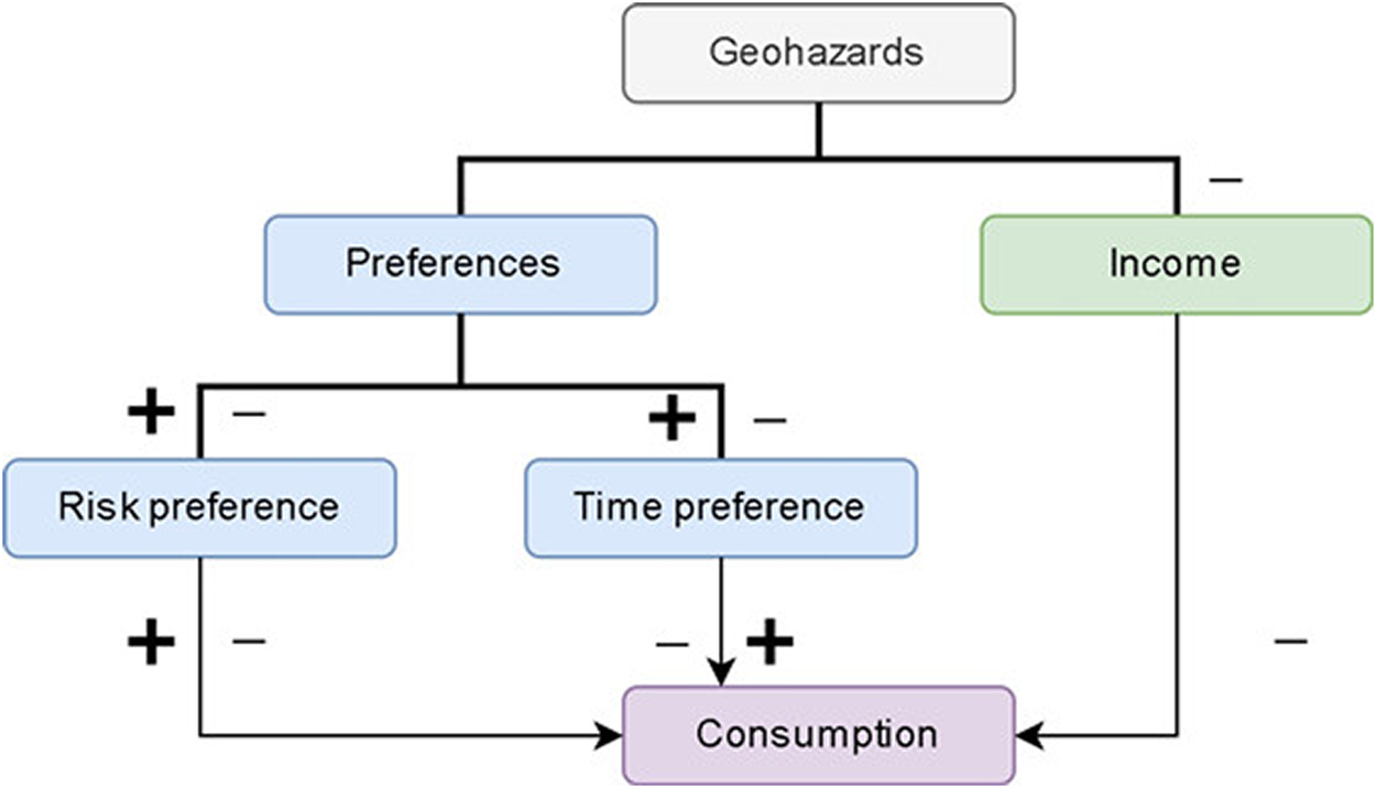
The third idea is that disaster experience affects consumption by reducing income (Mottaleb et al., 2013; Mertens et al., 2016). Both those who worked as self-employed, such as farmers, and on a wage were more likely to suffer reduced income after the disaster. However, other scholars found that disaster experience had no significant impact on income but on financial hardship and risk aversion (Johar et al., 2022). Based on the above research, the mechanism of geohazards on household consumption is shown in Figure 1.
FIGURE 1
Mechanism of geohazards on household consumption behavior.
Academic research on the impact of geohazards on consumer behavior is currently limited by the availability of data, and there is still much room for development. Firstly, most of the relevant research objects are restricted to specific disasters. To go beyond that, this paper uses the generalized geohazards data in China, and the research conclusions are more universally applicable. Secondly, most of the relevant studies only focused on the impact based on one mechanism, while this paper comprehensively tests three mechanism channels of the impact of disaster experience on consumption and provides micro evidence from Chinese households’ perspective. Thirdly, the empirical analysis of this paper uses Chinese household microdata, discusses and solves potential endogenous issues, and performs multidimensional robust tests and heterogeneity analysis to increase the reliability of the results. Besides the three theoretical and empirical aspects above, on a practical aspect, the outbreak of COVID-19 has been a huge shock to the global economy, and the findings of this paper could help predict the impact of this pandemic on households time preferences, risk preferences and consumption.
The remainder of this study is arranged as follows. The second section is the theoretical model, the third section is the econometrics model, data sources and descriptive statistics, the fourth section is the empirical tests, and the last is the conclusion section.
Theoretical Model
The existing consumption models have well-established the representations of time preference inconsistency, and this paper draws on the work of Phelps and Pollak (1968) and Krusell et al. (2002). However, there is a lack of authoritative expressions of changes in risk preferences. In order to find an analytical solution, this paper uses the common CARA function to describe the consumer utility function, that is , where θ is the absolute risk aversion factor.
Based on the research of Phelps and Pollak (1968) and Krusell et al. (2002), this paper sets the discount factor of consumers as {1, βδ, βδ2… βδt}. Then introducing the hyperbolic discounting model into the utility function:
Among them, the long-term discount factor used between the future T period and T+1 period (long-term) is . The short-term discount factor between period 0 and period 1 (short term) is βδ. β=1 represents the exponential discount function in which consumers have time consistency. β<1 represents short-term impatience of the consumer, lack of patience compared to the original plan and overspending relative to the original plan. β>1 means that consumers are more tolerant, more patient than the original plan, and spend less than the original plan.
Then the intertemporal decision-making of consumers can be expressed as the following dynamic programming problem:where β is the short-term discount factor and δ is the long-term discount factor used to express time preference inconsistency. yt is disposable income, at is household wealth, r is the interest rate, represents the income shock, obeys the normal distribution with the mean value of 0 and the variance of , and the instantaneous utility function of consumers is .
By establishing the Behrman equation, the optimal consumption is:
This optimal consumption shows that the change in household income, time preference and uncertainty of future income affect household consumption, which is consistent with the possible mechanism of previous literature. The disposable income yt and household wealth at, is positively correlated with consumer current spending ct. The variance of expected future income , which means uncertainty of future income, is negatively correlated with the current consumption ct. From the perspective of time preference, in contrast to no inconsistency in time preference that β=1, consumption increases when consumers are impatient that β<1, and decreases when β>1 consumers are more patient. The theoretical conclusion indicates the possible consequence of income, time preference and uncertainty on consumption. Empirical tests will further study the impact of geohazards on consumption through those variables.
Econometrics Model, Data and Descriptive Statistics
Econometrics Model
Based on the above ideas, the following econometric model is constructed to test the impact of geohazards on residents’ consumption.Where cij is the consumption of household i in region j, Zi represents other factors that may affect consumption, including household head characteristics and household characteristics. Xj is the control variable at the macro level.
The data in this paper comes from the China Household Finance Survey 2017 and the China National Bureau of Statistics in 2016, respectively conducted by the Southwestern University of Finance and Economics in 2017 (CHFS 2017) and the Chinese government. The CHFS 2017 sample covers 29 provinces (autonomous regions and municipalities) in China except for Xinjiang, Tibet, Hong Kong, Macao and Taiwan. In 2017, China Household Finance Survey collected 40,011 valid samples. The questionnaire questions covered the interviewees’ income, consumption, subjective preferences and other specific conditions of the participants in 2016, with national, provincial and sub-provincial city representation. The China National Bureau of Statistics provides provincial-level data.
Variable Selection and Descriptive Statistics
Household consumption variable includes total household consumption, categorized consumption expenditure and annual credit card spending. In testing the mechanism of the influence of geohazard experience on household consumption choice, the amount of annual credit card spending is selected as the measurement variable of household time preference for the reason that the credit card usage represents the household attitude between immediate utility and expected future utility (Meier and Sprenger, 2010; Gathergood, 2012).
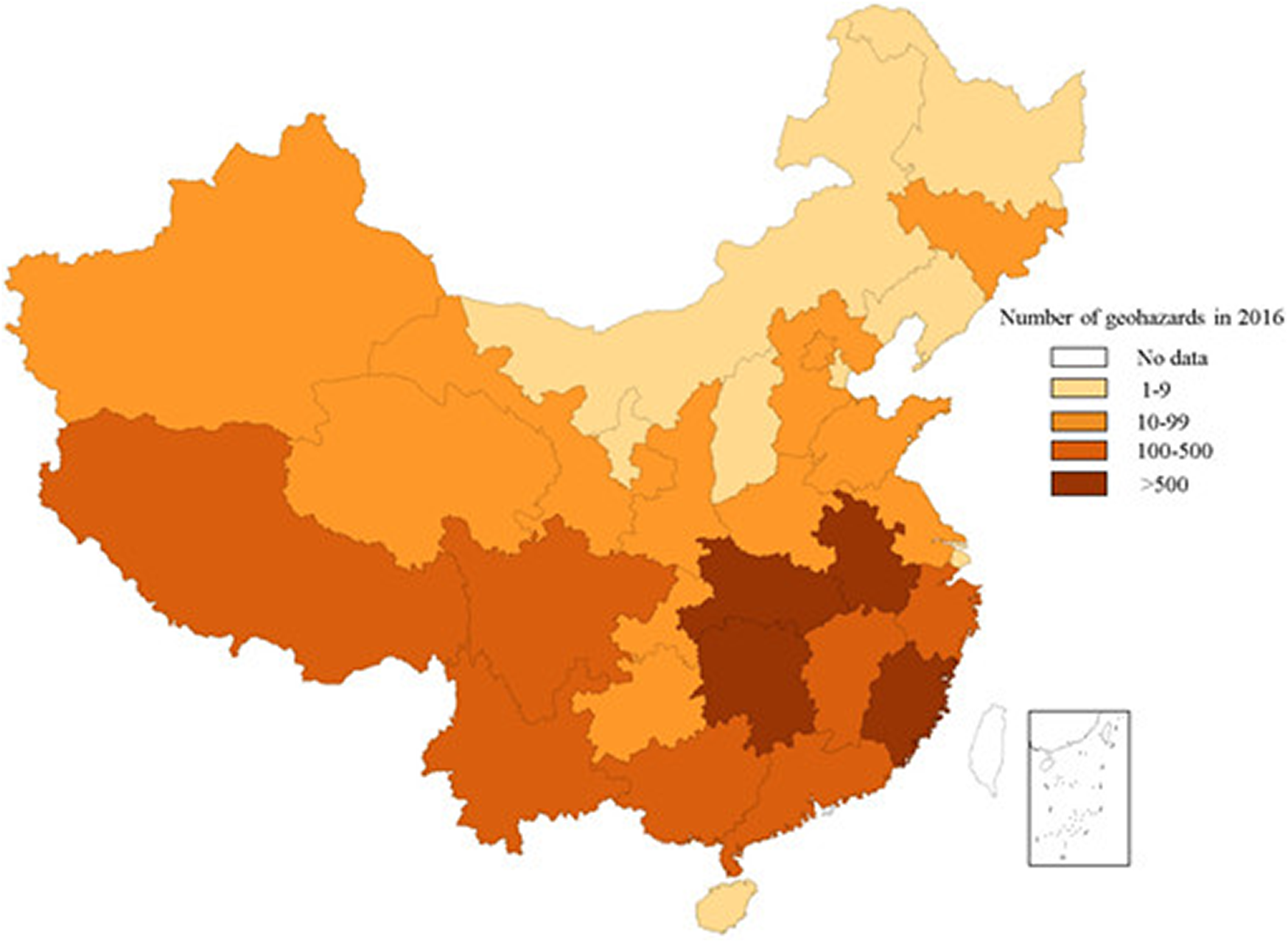
As for the geohazards variable, the frequency of provincial geological hazards is used as the measurement variable of the degree of geological disasters in the region. The number of casualties of provincial geological disasters is used as the robust test. In the China National Bureau of Statistics, geohazards refer to sudden geological hazards such as landslides, avalanches, mudslides, ground subsidence and slow-varying geological hazards such as ground cracks, ground subsidence and seawater intrusion. Figure 2 displays the geographic dispersion of frequency of geohazards.
FIGURE 2
Geographic dispersion of the number of geohazards.
Referring to the previous literature, control variables include household characteristics, household head characteristics, and macro control variables. Where household characteristics include annual household income, assets, whether the household lives in rural, whether the household owns houses, family size, and dependency ratio. The characteristics of a head of household include gender, age, square item of age, whether to pay medical insurance or endowment insurance, education level and marital status. Macro variables are provincial GDP, population and local fiscal general public expenditure.
In order to reduce the influence of extreme value on the results, this paper uses 99% quantile to deal with the extreme value of variables and takes the logarithm of non-dummy variables to reduce the influence of heteroscedasticity. Descriptive statistics of main variables are shown in Table 1.
TABLE 1
| Observations | Mean | Std. Dev | Min | Max | |
|---|---|---|---|---|---|
| total consumption | 40,011 | 65,337.565 | 83,908.3460 | 736.8 | 3,434,645 |
| hazard freq | 40,011 | 415.4377 | 930.7913 | 1 | 4,478 |
| hazard casualties | 40,011 | 18.9516 | 23.9163 | 0 | 84 |
| total income | 40,011 | 88,264.781 | 109,250.3346 | -1,068 | 690,180 |
| total asset | 40,011 | 1,055,887.7 | 1,785,408.3507 | 1,580 | 10,220,302 |
| age | 39,992 | 55.1923 | 14.0989 | 24 | 86 |
| family size | 40,011 | 3.1657 | 1.5170 | 1 | 8 |
| support rate | 40,011 | 0.3320 | 0.3439 | 0 | 1 |
| married | 39,966 | 0.8528 | 0.3543 | 0 | 1 |
| edugrp 2 | 39,958 | 0.2693 | 0.4436 | 0 | 1 |
| edugrp 3 | 39,958 | 0.0847 | 0.2785 | 0 | 1 |
| rural household | 40,011 | 0.3182 | 0.4658 | 0 | 1 |
| female | 40,010 | 0.2067 | 0.4050 | 0 | 1 |
| insurance pension | 39,683 | 0.8208 | 0.3835 | 0 | 1 |
| insurance medicine | 39,678 | 0.9332 | 0.2497 | 0 | 1 |
| own houses | 39,972 | 0.9044 | 0.2940 | 0 | 1 |
| gdp | 40,011 | 31,807.8040 | 22,250.4533 | 2,258.200 | 82,163.2030 |
| population | 40,011 | 5,448.4684 | 3,072.8354 | 582 | 11,908 |
| public expenditure | 40,011 | 514.0853 | 273.3921 | 75.79 | 1,147.35 |
| Rdls | 40,011 | 0.8439 | 0.9548 | 0.0044 | 4.3263 |
| the Han nationality | 25,983 | 0.9358 | 0.2451 | 0 | 1 |
The statistics description of main variables.
Empirical Results and Discussion
Analysis of Basic Results and Robust Tests
Table 2 displays the OLS basic results and a series of robust test results of the impact of geological hazard frequency on household consumption.
TABLE 2
| Variables | (1) | (2) | (3) | (4) | (5) |
|---|---|---|---|---|---|
| ln_total_consumption | ln_total_consumption | ln_total_consumption | ln_total_consumption | ln_total_consumption | |
| ln_hazard_freq | 0.0122*** | — | 0.0121*** | 0.0112*** | 0.0166*** |
| (0.0018) | — | (0.0018) | (0.0018) | (0.0035) | |
| ln_hazard_casualties | — | 0.0281*** | — | — | — |
| — | (0.0020) | — | — | — | |
| relief | — | — | 0.1156** | — | — |
| — | — | (0.0518) | — | — | |
| Rdls | — | — | — | 0.0101** | — |
| — | — | — | (0.0042) | — | |
| the Han nationality | — | — | — | — | 0.0172 |
| — | — | — | — | (0.0237) | |
| ln_total_income | 0.0909*** | 0.0908*** | 0.0909*** | 0.0909*** | 0.0886*** |
| (0.0036) | (0.0036) | (0.0036) | (0.0036) | (0.0066) | |
| ln_total_asset | 0.1549*** | 0.1551*** | 0.1551*** | 0.1548*** | 0.1535*** |
| (0.0027) | (0.0027) | (0.0027) | (0.0027) | (0.0052) | |
| age | -0.0210*** | -0.0204*** | -0.0211*** | -0.0208*** | -0.0199*** |
| (0.0018) | (0.0018) | (0.0018) | (0.0018) | (0.0041) | |
| age_2 | 0.0001*** | 0.0001*** | 0.0001*** | 0.0001*** | 0.0001*** |
| (0.0000) | (0.0000) | (0.0000) | (0.0000) | (0.0000) | |
| fami_size | 0.1145*** | 0.1138*** | 0.1145*** | 0.1146*** | 0.1141*** |
| (0.0026) | (0.0025) | (0.0026) | (0.0026) | (0.0049) | |
| support_r | -0.0470*** | -0.0456*** | -0.0471*** | -0.0471*** | -0.0488* |
| (0.0129) | (0.0129) | (0.0129) | (0.0129) | (0.0251) | |
| Married | 0.1496*** | 0.1509*** | 0.1498*** | 0.1496*** | 0.1381*** |
| (0.0111) | (0.0111) | (0.0111) | (0.0111) | (0.0222) | |
| edugrp_2 | 0.1543*** | 0.1556*** | 0.1544*** | 0.1550*** | 0.1451*** |
| (0.0078) | (0.0078) | (0.0078) | (0.0078) | (0.0148) | |
| edugrp_3 | 0.2937*** | 0.2942*** | 0.2937*** | 0.2942*** | 0.2893*** |
| (0.0130) | (0.0129) | (0.0130) | (0.0129) | (0.0280) | |
| Rural | -0.2930*** | -0.2943*** | -0.2937*** | -0.2933*** | -0.2994*** |
| (0.0084) | (0.0084) | (0.0084) | (0.0084) | (0.0153) | |
| female | 0.0569*** | 0.0563*** | 0.0570*** | 0.0564*** | 0.0483*** |
| (0.0086) | (0.0086) | (0.0086) | (0.0086) | (0.0169) | |
| insur_pension | -0.0090 | -0.0068 | -0.0090 | -0.0096 | -0.0063 |
| (0.0094) | (0.0094) | (0.0094) | (0.0094) | (0.0186) | |
| insur_med | 0.0285** | 0.0270* | 0.0284** | 0.0284** | 0.0012 |
| (0.0140) | (0.0139) | (0.0140) | (0.0139) | (0.0287) | |
| House | -0.3491*** | -0.3478*** | -0.3493*** | -0.3492*** | -0.2922*** |
| (0.0127) | (0.0127) | (0.0127) | (0.0127) | (0.0258) | |
| ln_gdp_prov | 0.1219*** | 0.1489*** | 0.1212*** | 0.1367*** | 0.1617*** |
| (0.0107) | (0.0108) | (0.0107) | (0.0122) | (0.0192) | |
| ln_popu_prov | -0.3308*** | -0.3114*** | -0.3305*** | -0.3280*** | -0.2961*** |
| (0.0159) | (0.0160) | (0.0159) | (0.0159) | (0.0289) | |
| ln_ public_prov | 0.1770*** | 0.1185*** | 0.1779*** | 0.1606*** | 0.0657 |
| (0.0227) | (0.0229) | (0.0228) | (0.0237) | (0.0407) | |
| Constant | 8.7481*** | 8.6506*** | 8.7480*** | 8.6674*** | 8.6857*** |
| (0.0761) | (0.0759) | (0.0761) | (0.0831) | (0.1543) | |
| Observations | 39,342 | 39,342 | 39,342 | 39,342 | 10,976 |
| R-squared | 0.4606 | 0.4627 | 0.4607 | 0.4607 | 0.4514 |
Impact of geological hazard frequency on household consumption.
Standard error in parentheses; *, **, *** denote statistical significance levels at 10, 5, and 1%, respectively.
Table 2 regression 1) reports the effect of provincial geohazard frequency on total household consumption in 2016. The results show that when other conditions remain unchanged, a 1% increase in the frequency of geological disasters will promote the total consumption of households by 1.22%. This result is significant at the statistical level of 1%.
Take Table 2 regression 1) as an example to explain the effect of control variables on consumption. Household assets and income have a significant positive impact on consumption, which is consistent with the conclusion of classical economic theory. The age of the household head has an inverted U-shaped relationship with consumption, with consumption showing an upward movement and then a downward trend as age increases. Family size has a significant positive effect on total household consumption. The proportion of family support has a negative inhibitory effect on family consumption. Married or cohabiting households spend significantly more compared to households in other marital status. The higher the education level of the head of household, the higher the family’s expectation of future income. With the increase of expectation permanent income, household consumption will consequently increase significantly. There are differences in consumption between rural and urban families in China, which shows that the consumption of rural families is lower than that of urban families. Households headed by women consume more. If the head of household has medical insurance or endowment insurance, it will reduce the motivation for preventive savings and promote family consumption, but the role of endowment insurance in promoting family consumption is not significant. Households that own their own houses will have lower consumption. The more developed the economy of the province, the more government public expenditure, the higher the level of household total consumption, and the population of the province is negatively correlated with the total household consumption.
Further empirical tests reveal that the above results passed the robust tests based on the replacement of explanatory variables and the empirical tests to mitigate the endogenous problem of omitted variables, that is, the results of regression 2) to regression 5) in Table 2. Among them, regression 2) is a robust test based on the replacement of explanatory variables. Replacing the explanatory variable with the number of casualties due to geohazards, the results confirm that the deeper the area is affected by geohazards, the higher the level of total household consumption and the total household consumption level increases statistically significant at the 1% level. Table 2 Regression 3) to regression 5) is to reduce the endogenous problem of missing variables. The impact on consumption in disaster areas may be uncertain due to the compensation effect of receiving government disaster relief funds based on the income level. In order to distinguish between the effects of receiving disaster relief funds and the degree of geological disaster on consumption, the dummy variable of whether the family received government disaster relief funds in that year was added to the regression (3). The results show that the promotion effect of disaster relief funds on consumption does not change the significance of the care variable coefficient of regional geohazards frequency on household consumption. Areas with different frequencies of geohazards may have different geographical environments or cultural backgrounds, and they may affect the consumption level. Table 2 regression 4) uses the topographic relief degree of the province as the proxy variable of the geographical environment and Table 2 regression 5) uses the Han nationality dummy as the proxy variable of the cultural differences. After adding those variables, the coefficient of the core explanatory variable remains robust.
Heterogeneity analysis
Tables 3, 4 analyze the heterogeneity of household consumption structure and different income groups.
TABLE 3
| Variables | (1) | (2) | (3) | (4) |
|---|---|---|---|---|
| ln_food_c | ln_clothing_c | ln_resident_c | ln_equipment_c | |
| ln_hazard_freq | 0.0335*** | 0.0288*** | -0.0109*** | 0.0238*** |
| (0.0018) | (0.0063) | (0.0038) | (0.0043) | |
| Control variables | Yes | Yes | yes | yes |
| Observations | 39,342 | 39,342 | 39,342 | 39,342 |
| R-squared | 0.3825 | 0.3416 | 0.2404 | 0.2893 |
| Variables | (5) | (6) | (7) | (8) |
| ln_medical_c | ln_travel_c | ln_educ_c | ln_other_c | |
| ln_hazard_freq | -0.0588*** | 0.0150*** | -0.0424*** | -0.0049 |
| (0.0094) | (0.0034) | (0.0099) | (0.0055) | |
| Control variables | Yes | yes | Yes | yes |
| Observations | 39,342 | 39,342 | 39,342 | 39,342 |
| R-squared | 0.0638 | 0.4120 | 0.3365 | 0.0277 |
Heterogeneity of the frequency of geohazards in the category of consumption.
Standard error in parentheses; *, **, *** denote statistical significance levels at 10, 5, and 1%, respectively.
TABLE 4
| Dependent variable: ln_wtotal_consump | (1) | (2) | (3) | (4) |
|---|---|---|---|---|
| Lowest 25% | 25–50% | 50–75% | Top 25% | |
| ln_hazard_freq | 0.0153*** | 0.0197*** | 0.0121*** | -0.0008 |
| (0.0036) | (0.0033) | (0.0032) | (0.0035) | |
| Control variables | Yes | Yes | yes | yes |
| Observations | 9,806 | 9,816 | 9,866 | 9,854 |
| R-squared | 0.4610 | 0.3908 | 0.3650 | 0.3540 |
The impact of frequency of geohazards on household consumption at different income levels.
Standard error in parentheses; *, **, *** denote statistical significance levels at 10, 5, and 1%, respectively.
Table 3 shows the heterogeneous impact of the frequency of geological disasters on eight types of consumption. According to the estimation results in Table 3, the frequency of geological disasters will significantly promote the consumption types of food, clothing, household equipment and services, transportation and communication. The type of consumption of housing, health care and education, culture and entertainment services are significantly suppressed, and the effect on other categories of consumption is not significant. Overall, the results of heterogeneity analysis support the conclusion of baseline regression and suggest that geological hazards affect the structure of household consumption.
In order to explore whether the consumption of households at different income levels differs according to their wealth traits, Table 4 reports the impact of the frequency of geohazards on household consumption at different income levels. Considering the differences in the level of economic development of each province, we classified the full sample households into four groups in descending order of per capita income within their respective provinces. The lowest 25% of households ranked in terms of per capita income are considered low-income households, households ranked 25–50% are regarded as lower-middle-income households, households ranked 50–75% are considered upper-middle-income households, and households with per capita income ranked the highest 25% are regarded as high-income households. The results of Table 4 show that for families at different income levels, the impact of the frequency of geological disasters on their current consumption is different. The promotion effect of geological disaster frequency on the consumption of low-income and lower-middle-income households is higher than that of upper-middle-income and high-income groups, among which the promotion effect on the consumption of lower-middle-income households is the strongest. The promotion effect on the consumption of high-income families is not significant.
Mechanism Analysis
This paper discusses the impact mechanism of the frequency of geological disasters on household consumption from the perspective of income, risk preference and time preference, as well as discuss the long-term impact of the frequency of geological disasters on household consumption.
According to the conclusions of the theoretical model, household consumption is positively influenced by income. The frequency of geological disasters has an impact on income in two directions. On one hand, due to the occurrence of disasters, the possibility of income decline or unemployment increases (Berlemann and Eurich, 2021), causing a decrease in household income. On the other hand, the hazard relief funds issued by the government can make up for the decline in income. Post-disaster construction assistance and relief work can drive employment and investment to a certain extent in the affected areas, with a positive effect on the income of households. We need to test whether the frequency of geological disasters will affect the income level of affected families. The results of regression 1) in Table 5 show that the frequency of geological hazards has no significant effect on household income level. This indicates that the change in income level is not a mechanism by which the frequency of geohazards affects household consumption.
TABLE 5
| Variables | (1) | (2) | (3) | (4) |
|---|---|---|---|---|
| ln_total_income | risk_aversion | ln_credit_c | ln_total_c | |
| ln_hazard_freq | 0.0082 | -0.0036 | 0.0891*** | 0.0074*** |
| (0.0052) | (0.0042) | (0.0271) | (0.0027) | |
| — | — | — | 0.0066** | |
| — | — | — | (0.0028) | |
| Control variables | Yes | Yes | yes | yes |
| Observations | 24,824 | 35,089 | 1,389 | 39,342 |
| R-squared | 0.2480 | — | — | 0.4607 |
Mechanism analysis and long-term impact test.
Standard error in parentheses; *, **, *** denote statistical significance levels at 10, 5, and 1%, respectively.
According to the precautionary saving theory, the higher the degree of risk aversion of residents, the more inclined they are to increase current savings to smooth future consumption, leading to a reduction of current consumption. On the contrary, the lower the level of risk aversion in the household, the fewer savings are made for precautionary motives and the weaker inhibition effect on current consumption. Therefore, we test whether the frequency of geohazards affects consumption by changing affected residents’ risk preferences. According to the CHFS questionnaire on the measurement of risk preference, that is, ‘If you had two lottery tickets to choose from right now and if you choose the first one, you have a 100% chance of getting 4,000 yuan, if you choose the second one, you have a 50% chance of getting 10,000 yuan, and 50% chance of getting nothing, which one would you like to choose?’ In this paper, the risk aversion dummy variable is set to one for respondents who choose the first lottery ticket, and the risk aversion dummy variable is set to 0 for a respondent who chooses the second lottery ticket. The results of regression 2) in Table 5 show that the frequency of geohazards has no significant impact on household risk preference, indicating that the change of risk preference is not the mechanism of the frequency of geohazards affecting household consumption.
Time preference is an important factor influencing individuals’ intertemporal decisions; individuals with long-term time preference have higher utility for future consumption and are more inclined to increase savings and decrease consumption in the current period. In contrast, individuals with short-term time preferences are more likely to increase current consumption and reduce savings. This paper tests whether the frequency of geological hazards changes the temporal preferences of affected residents. Credit card expenditure, which is closely related to time preference, is selected as the proxy variable of time preference. Since credit card expenditure can only be observed by using credit cards, the observed value of credit card consumption of households without credit cards is 0, resulting in truncated data, so Tobit regression is used. Table 5 regression 3) shows that the frequency of geohazards has a significant positive effect on the amount of credit card spending. This suggests that the frequency of geohazards may be a mechanism for households to increase their consumption by changing individual time preferences to place more emphasis on the utility of current consumption, which in turn promotes household current consumption. Changing the time preference may be a mechanism for families to increase consumption after geological disasters experience.
Table 5 regression four adds the provincial geohazard frequency variable with a 5-years lag to test the long-term effect of geohazard frequency on household consumption. The regression results show that experiencing a geological disaster not only has an immediate and significant boosting effect on residents’ consumption but also has a significant long-term boosting effect on their consumption.
Conclusion
Geological hazards have a significant impact on consumer behavior, but few previous studies have focused on the impact of generalized geohazards on consumption and conducted multi-perspective mechanism discussions. Moreover, the existing literature has not reached a consensus conclusion. To address this research gap, this paper examines how geohazards in China affect household consumption by using CHFS 2017 microdata and the National Bureau of Statistics provincial-level data. Based on the above theoretical model and empirical test results, the conclusions reached in this study are as follows:
Firstly, the level of household consumption is significantly higher in regions with more geohazards. The results remain robust after changing the explanatory variables, excluding the impact of government disaster relief funds and solving the endogenous problems that may be brought by different geographical environments or cultural backgrounds.
Secondly, a more detailed heterogeneity analysis reveals that geohazards affect the consumption structure of households, with significant increases in consumption categories such as food, clothing, household equipment supplies and services, transportation and communication consumption types. In addition, the frequency of geological hazards affects households’ consumption at different income-level to different degrees, with a stronger consumption boost for low-income and lower-middle-income households. In addition, the empirical results also confirm that the frequency of geohazards has a significant increase impact on household consumption not only in the short term but also in the long term.
Thirdly, the empirical results show that the impact mechanism of the frequency of geohazards on household consumption mainly lies in changing the individual’s time preference, making the individual prone to indulge in the present and increase the current consumption. While income and risk attitudes do not change significantly after geohazards and are not the influencing mechanisms.
Statements
Data availability statement
The original contributions presented in the study are included in the article/Supplementary material, further inquiries can be directed to the corresponding author.
Author contributions
BZ contributed to conception and design of the study. LZ performed the statistical analysis and wrote the first draft of the manuscript. All authors contributed to manuscript revision, read, and approved the submitted version.
Funding
This study is supported by the 1. Research Center for Finance and Enterprise Innovation, Hebei University of Economics and Business; 2. Scientific Research and Development Program Fund of Hebei University of Economics and Business (2021ZD11).
Conflict of interest
The authors declare that the research was conducted in the absence of any commercial or financial relationships that could be construed as a potential conflict of interest.
Publisher’s note
All claims expressed in this article are solely those of the authors and do not necessarily represent those of their affiliated organizations, or those of the publisher, the editors and the reviewers. Any product that may be evaluated in this article, or claim that may be made by its manufacturer, is not guaranteed or endorsed by the publisher.
References
1
Alam E. Ray-Bennett N. S. (2021). Disaster Risk Governance for District-Level Landslide Risk Management in Bangladesh. Int. J. Disaster Risk Reduct.59, 102220. 10.1016/j.ijdrr.2021.102220
2
Berlemann M. Eurich M. (2021). Natural Hazard Risk and Life Satisfaction - Empirical Evidence for Hurricanes. Ecol. Econ.190, 107194. 10.1016/j.ecolecon.2021.107194
3
Bourdeau-Brien M. Kryzanowski L. (2020). Natural Disasters and Risk Aversion. J. Econ. Behav. Organ.177, 818–835. 10.1016/j.jebo.2020.07.007
4
Burrows K. Desai M. U. Pelupessy D. C. Bell M. L. (2021). Mental Wellbeing Following Landslides and Residential Displacement in Indonesia. SSM - Ment. Health1, 100016. 10.1016/j.ssmmh.2021.100016
5
Callen M. (2015). Catastrophes and Time Preference: Evidence from the Indian Ocean Earthquake. J. Econ. Behav. Organ.118, 199–214. 10.1016/j.jebo.2015.02.019
6
Cameron L. Shah M. (2015). Risk-taking Behavior in the Wake of Natural Disasters. J. Hum. Resour.50 (2), 484–515.
7
Cassar A. Healy A. von Kessler C. (2017). Trust, Risk, and Time Preferences after a Natural Disaster: Experimental Evidence from Thailand. World Dev.94, 90–105. 10.1016/j.worlddev.2016.12.042
8
Chantarat S. Oum S. Samphantharak K. Sann V. (2019). Natural Disasters, Preferences, and Behaviors: Evidence from the 2011 Mega Flood in Cambodia. J. Asian Econ.63, 44–74. 10.1016/j.asieco.2019.05.001
9
Eckel C. C. El-Gamal M. A. Wilson R. K. (2009). Risk Loving after the Storm: A Bayesian-Network Study of Hurricane Katrina Evacuees. J. Econ. Behav. Organ.69, 110–124. 10.1016/j.jebo.2007.08.012
10
Gathergood J. (2012). Self-control, Financial Literacy and Consumer Over-indebtedness. J. Econ. Psychol.33, 590–602. 10.1016/j.joep.2011.11.006
11
Isoré M. Szczerbowicz U. (2017). Disaster Risk and Preference Shifts in a New Keynesian Model. J. Econ. Dyn. Control79, 97–125. 10.1016/j.jedc.2017.04.001
12
Johar M. Johnston D. W. Shields M. A. Siminski P. Stavrunova O. (2022). The Economic Impacts of Direct Natural Disaster Exposure. J. Econ. Behav. Organ.196, 26–39. 10.1016/j.jebo.2022.01.023
13
Krusell P. Kuruşçu B. Smith A. A. (2002). Time Orientation and Asset Prices. J. Monetary Econ.49, 107–135. 10.1016/S0304-3932(01)00095-2
14
Li X. Huang X. Zhang Y. (2021). Spatio-temporal Analysis of Groundwater Chemistry, Quality and Potential Human Health Risks in the Pinggu Basin of North China Plain: Evidence from High-Resolution Monitoring Dataset of 2015-2017. Sci. Total Environ.800, 149568. 10.1016/j.scitotenv.2021.149568
15
Meier S. Sprenger C. (2010). Present-Biased Preferences and Credit Card Borrowing. Am. Econ. J. Appl. Econ.2, 193–210. 10.1257/app.2.1.193
16
Mertens K. Jacobs L. Maes J. Kabaseke C. Maertens M. Poesen J. et al (2016). The Direct Impact of Landslides on Household Income in Tropical Regions: A Case Study from the Rwenzori Mountains in Uganda. Sci. Total Environ.550, 1032–1043. 10.1016/j.scitotenv.2016.01.171
17
Moniruzzaman S. (2019). Income and Consumption Dynamics after Cyclone Aila: How Do the Rural Households Recover in Bangladesh?Int. J. Disaster Risk Reduct.39, 101142. 10.1016/j.ijdrr.2019.101142
18
Mottaleb K. A. Mohanty S. Hoang H. T. K. Rejesus R. M. (2013). The Effects of Natural Disasters on Farm Household Income and Expenditures: A Study on Rice Farmers in Bangladesh. Agric. Syst.121, 43–52. 10.1016/j.agsy.2013.06.003
19
Page L. Savage D. A. Torgler B. (2014). Variation in Risk Seeking Behaviour Following Large Losses: A Natural Experiment. Eur. Econ. Rev.71, 121–131. 10.1016/j.euroecorev.2014.04.009
20
Pham N. T. T. Nong D. Garschagen M. (2021). Natural Hazard's Effect and Farmers' Perception: Perspectives from Flash Floods and Landslides in Remotely Mountainous Regions of Vietnam. Sci. Total Environ.759, 142656. 10.1016/j.scitotenv.2020.142656
21
Phelps E. S. Pollak R. A. (1968). On Second-Best National Saving and Game-Equilibrium Growth. Rev. Econ. Stud.35, 185–199. 10.2307/2296547
22
Rosenbaum M. S. Culshaw M. G. (2003). Communicating the Risks Arising from Geohazards. J. R. Stat. Soc. A166, 261–270. 10.1111/1467-985x.00275
23
Salvati P. Petrucci O. Rossi M. Bianchi C. Pasqua A. A. Guzzetti F. (2018). Gender, Age and Circumstances Analysis of Flood and Landslide Fatalities in Italy. Sci. Total Environ.610-611, 867–879. 10.1016/j.scitotenv.2017.08.064
24
Sapkota J. B. (2018). Human Well-Being after 2015 Nepal Earthquake: Micro-evidence from One of the Hardest Hit Rural Villages. Munich, Germany: MPRA Paper.
25
Shinohara Y. Kume T. (2022). Changes in the Factors Contributing to the Reduction of Landslide Fatalities between 1945 and 2019 in Japan. Sci. Total Environ.827, 154392. 10.1016/j.scitotenv.2022.154392
26
Voors M. Nillesen E. Verwimp P. Bulte E. Lensink R. Van Soest D. (2012). Violent Conflict and Behavior: A Field Experiment in Burundi. Am. Econ. Rev.102 (2), 941–964.
27
Yang H.-Q. Zhang L. Gao L. Phoon K.-K. Wei X. (2022). On the Importance of Landslide Management: Insights from a 32-year Database of Landslide Consequences and Rainfall in Hong Kong. Eng. Geol.299, 106578. 10.1016/j.enggeo.2022.106578
28
Yao D. Xu Y. Zhang P. (2019). How a Disaster Affects Household Saving: Evidence from China's 2008 Wenchuan Earthquake. J. Asian Econ.64, 101133. 10.1016/j.asieco.2019.101133
29
Yao R. Yan Y. Wei C. Luo M. Xiao Y. Zhang Y. (2022). Hydrochemical Characteristics and Groundwater Quality Assessment Using an Integrated Approach of the PCA, SOM, and Fuzzy C-Means Clustering: A Case Study in the Northern Sichuan Basin. Front. Environ. Sci.10. 10.3389/fenvs.2022.907872
30
Zhang Y. Dai Y. Wang Y. Huang X. Xiao Y. Pei Q. (2021a). Hydrochemistry, Quality and Potential Health Risk Appraisal of Nitrate Enriched Groundwater in the Nanchong Area, Southwestern China. Sci. Total Environ.784, 147186. 10.1016/j.scitotenv.2021.147186
31
Zhang Y. He Z. Tian H. Huang X. Zhang Z. Liu Y. et al (2021b). Hydrochemistry Appraisal, Quality Assessment and Health Risk Evaluation of Shallow Groundwater in the Mianyang Area of Sichuan Basin, Southwestern China. Environ. Earth Sci.80, 576. 10.1007/s12665-021-09894-y
Summary
Keywords
geohazards, time preference, risk preference, income, household consumption
Citation
Zhao L and Zhu B (2022) How do Geohazards Affect Household Consumption: Evidence From China. Front. Earth Sci. 10:941948. doi: 10.3389/feart.2022.941948
Received
12 May 2022
Accepted
24 June 2022
Published
18 July 2022
Volume
10 - 2022
Edited by
Yunhui Zhang, Southwest Jiaotong University, China
Reviewed by
Canlin Xu, Guizhou University of Finance and Economics, China
Ying Zhou, Guangdong University of Finance and Economics, China
Updates
Copyright
© 2022 Zhao and Zhu.
This is an open-access article distributed under the terms of the Creative Commons Attribution License (CC BY). The use, distribution or reproduction in other forums is permitted, provided the original author(s) and the copyright owner(s) are credited and that the original publication in this journal is cited, in accordance with accepted academic practice. No use, distribution or reproduction is permitted which does not comply with these terms.
*Correspondence: Boyi Zhu, 2019000464@ruc.edu.cn
This article was submitted to Geohazards and Georisks, a section of the journal Frontiers in Earth Science
Disclaimer
All claims expressed in this article are solely those of the authors and do not necessarily represent those of their affiliated organizations, or those of the publisher, the editors and the reviewers. Any product that may be evaluated in this article or claim that may be made by its manufacturer is not guaranteed or endorsed by the publisher.