Model structure and ensemble size: Implications for predictions of groundwater age

1 Introduction

Groundwater accounts for approximately 97% of all accessible fresh water, supplies drinking water for nearly half the world’s population, and accounts for 43% of the global water consumption for agriculture (Siebert et al., 2010; Guppy et al., 2018). Physically based numerical models (as opposed to data-driven models such as are used in Ruidas et al., 2021. or Jaydhar et al., 2022), combined with subsurface properties inferred from sparse observations can help extend our understanding of groundwater systems (e.g., Singh, 2014), providing an essential tool to help inform resource management decisions (Jakeman et al., 2016). However, all models require simplification of real-world properties and processes. Identifying the appropriate level of simplification for modelling groundwater systems remains challenging. Appropriate simplification depends on the intended use of the model (Watson et al., 2013; Guthke, 2017; White, 2017). We explore this important issue in the context of simulating groundwater age at a national scale across Aotearoa/New Zealand, to inform national water management policy. Note, the objective of the study presented here is not to provide definitive maps for groundwater age across Aotearoa/New Zealand, but rather to explore and highlight the implications of model and methodological simplification on groundwater age predictions at large scale.

Groundwater age provides a convenient method for evaluating the potential for groundwater recharge and hence contamination from recent sources (Sanford 2011; Morgenstern et al., 2015). The utility of decision support models based on groundwater age, where “young” groundwater suggests a potential groundwater contamination risk and “old” groundwater suggests a smaller component of modern recharge, would clearly be compromised by the presence of model structural errors that bias simulated groundwater age (e.g., Knowling et al., 2020). This study reveals that predictions of groundwater age can be biased by the inability to represent parameter complexity with simplified (upscaled) layering. Due to the relationship between flow depth and groundwater age, where deeply circulating water is generally older, the range of ages impacted depends on the depth of these structural simplifications.

Increased and wide-spread human impacts on climate and natural resources can warrant national government consideration and oversight of environmental processes and resource management activities over larger spatial extents, often in data-scarce areas (e.g., Regan et al., 2019). Maintaining national oversite of the effectiveness of policy requires an understanding of the broad range of natural processes and resource management activities that affect water resources extending from the mountains to the sea. This understanding also includes consideration of interactions between climate, ecosystems, lakes, rivers, aquifers, land use, land management, and water allocation.

However, the desire for models with continuous coverage over large spatial scales presents several modelling challenges: 1) trade-offs between model resolution and computational burden, 2) upscaling of hydraulic properties to a representative elemental volume (REV; the volume within which properties are assumed to be constant to facilitate numerical modelling), 3) representation of local processes over a large REV (e.g., upscaling stream-aquifer interactions), 4) representation of high variations in permeability (e.g., bedrock–aquifer contacts which typically form model boundaries in “traditional” groundwater models), 5) large changes in topography (e.g., Southern Alps rising 3,700 km from sea level over 30 km and/or deeply incised streams), and 6) limited subsurface data makes characterization of the groundwater system difficult, especially in areas with complex topography and geology like Aotearoa/New Zealand. We explore these modelling challenges within this paper.

2 Background

2.1 Model structure and parameterization challenges

One of the most fundamental techniques for simplifying processes and properties in numerical groundwater models is the subdivision of the model domain into discrete volumes with representative properties (REV). This requires heterogeneous and potentially scale dependent properties (e.g., hydraulic conductivity, porosity) within each REV to be represented by a single value in each cell. Also, complex processes (e.g., stream-aquifer interactions) need to be conceptualized and simplified in a way that allows them to be effectively represented over the entire cell.

The choice of model discretization provides the underlying structure to support the parameter representation (parameterization) of hydraulic properties. It also imposes a limit on the level of parameterization a numerical groundwater model can accommodate for history matching and predictions. Coarse discretization can reduce the computational burden and may ease the parameter estimation and inversion process, but it also increases the potential for structural deficiencies caused by homogenising processes and properties over larger areas which can bias model results (e.g., Wildemeersch et al., 2014; Knowling et al., 2019).

Doherty and Moore (2021) discuss how the model structure, and the accompanying parameterization approach, need not be more detailed than is required to make the prediction of interest, despite resulting in a more abstract (less “realistic”) representation of hydraulic properties. On the other hand, parameter compensation resulting from deficiencies in structural and/or parameterization detail may impose bias in predictions, especially if those predictions are significantly different than data used for history matching (Doherty and Welter, 2010; Doherty and Christensen, 2011; White et al., 2014; Doherty, 2015). White et al. (2019a) explored the impact of truncating the vertical representation of a regional groundwater system, by comparing a 7-layer representation of a regional aquifer system, with truncated 2- and 4-layer representations. Knowling et al. (2020), showed that the inappropriate vertical truncation limited the ability of that model to assimilate information in tritium data, imposing a history matching induced parameter and predictive bias.

None of the previous work investigating the impact of model discretization on prediction uncertainty has specifically isolated the influence of vertical discretization/layering while keeping all other factors the same (e.g., aquifer thickness). This research specifically focusses on issues associated with using simplified vertical discretisation approaches to represent complex parameter fields and its impact on the uncertainty of groundwater age model predictions after history matching. We use a paired complex-simple model methodology to explore the propensity for bias using various vertical discretisation structures (Doherty and Christensen, 2011; White et al., 2019a; Gosses and Wöhling, 2019; Knowling et al., 2019).

In this study groundwater flow is simulated using MODFLOW and advective transport, used as a surrogate for age, is simulated using MODPATH (particle tracking). We show that the inability of the coarse discretization to represent the appropriate level of heterogeneity during the history matching process results in model bias when compared to more refined discretization schemes.

2.2 History matching challenges

Highly parameterized approaches to model inversion can provide the flexibility to match observations but can also incur a large computational cost when using finite difference methods, which require one model run per adjustable parameter to fill a sensitivity matrix (Jacobian). Here instead we use the iterative ensemble smoother (IES; Chen and Oliver, 2013) method as implemented in the PEST++ suite (White, 2018). The IES method calculates an empirical Jacobian based on an ensemble of stochastic realizations. The number of realizations in the ensemble is generally much less than the number of adjustable parameters, resulting in significant gains in computational efficiency (e.g., Hunt et al., 2021).

The size of the IES ensemble should reflect the dimensionality of the solution space (i.e., the extent to which history matching targets inform various parameters), and therefore it is problem dependent. Spurious correlations can compromise parameter upgrade calculations when the ensemble size is small compared to the number of independent observations that span the solution space. Determining the appropriate ensemble size is challenging in that it depends on the relationship between the history matching dataset, and the representation of relevant real-world detail in the model (e.g., discretization or resolution of the computational grid), the predictions of interest, and the scale of the processes being simulated. Systematic explorations of this issue appear to be absent in the literature.

This research explores the size of the stochastic ensembles used for history matching in IES. Smaller ensembles combined with simplified model structures compromise the predictive ability of the calibrated model, despite a simple, synthetic dataset used for history matching. In some cases, this compromise is exacerbated as a better fit to the calibration dataset is sought through more iterations. The automatic adaptive localization (Luo et al., 2018) option implemented in PEST++ is shown to improve history matching and prediction.

2.3 Research objectives

In Aotearoa/New Zealand groundwater accounts for nearly 70% of consented freshwater takes and supplies approximately 30% of the population with drinking water (White, 2001; Rajanayaka et al., 2010). Land use changes over the last 40-year have resulted in increased groundwater contamination (e.g., nitrogen, pathogens, etc) prompting a national scale evaluation of groundwater resources and threats (Ministry for the Environment and Stats, 2021). In responses to these changes the National Policy Statement for Freshwater Management in New Zealand (NPSFWM) calls for the management of freshwater in a way that gives effect to Te Mana o te Wai (“the fundamental importance of water and the recognition that protecting the health of freshwater protects the health and well-being of the wider environment”; Ministry for the Environment, 2020).

We present a series of national scale models (approximately 268,000 km²) that simulate groundwater flow and groundwater age (derived from particle tracking), embracing the extensive nature of New Zealand’s NPSFWM. These models use the best available nationwide data and estimates of uncertainty for groundwater recharge, hydrogeology, and the location of stream networks. This model represents the spatially continuous groundwater system in Aotearoa/New Zealand and a consistent starting point for the development of regional or local scale models that may include more detailed representation of the processes of interest. However, the complexity of the natural world and the spatial extent of this model require significant abstraction and simplification of many processes. This simplification is necessary to ensure numerical stability and reasonable simulation times that enable history matching and inversion. This study specifically investigates the uncertainty and bias imposed by simplification of model layering on predictions of groundwater age.

3 Methods

The models presented herein are designed to evaluate: 1) the effects of different vertical discretization approaches on simulations of particle travel times in large scale groundwater models and 2) the effects of ensemble size on the ability of the model to match predictions. The model calculates particle travel times from a surface water source (i.e., stream or rainfall recharge) to an observation location via backward particle tracking. We use these particle travel times as an estimate of groundwater age, which in turn can be used to infer the potential susceptibility of groundwater to contamination from recent surface sources (Stauffer et al., 2005) and estimate sustainable groundwater recharge rates (McMahon et al., 2011). Vertical discretization is explored using three layering schemes: up to 50 evenly spaced layers (“complex” model), up to four layers with fine discretization in the upper layers and a single layer at depth (“fine” model), and up to four layers with evenly spaced layers at depth (“even” model). See below for detailed descriptions.

The IES method is used to match model outputs to a synthetic dataset (i.e., “truth”) using models with alternative vertical discretization. One realization is chosen from a 300-member ensemble of the complex model to serve as the truth, based on the minimum sum of squared differences between the realization age at each location ($ag{e}_i$) and the simulated mean age at each observation location (${\overline{age}}_i$):

$\min {\displaystyle \sum }_i^n{\left(ag{e}_i-\overline{ag{e}_i}\right)}^2(1)$

where n is the number of observation locations in gravel and sand. The realization chosen to represent the truth is removed from the parameter ensembles used for history matching.

We consider a failure or conflict to occur if the true value of an observation (plus or minus a representative measurement noise) falls outside the range of the simulated observation ensemble. The percentage of locations for which the model fails to capture the truth (Pf) is the ratio of the number of observation (parameter) values that fail to total number of observations (parameters), times 100. This is the same approach used to identify prior data conflict (PDC) in PEST++ and requires no assumptions about the shape of the posterior probability density function (PDF). More thorough analysis of the PDFs and more precise statistical tests are warranted to determine criteria for model failure in real world applications with specific management objectives.

Simulating groundwater age older than the true age (“overestimation”) represents a failure of the model in a management context when groundwater age is used as a proxy for potential contamination from recent sources. Conversely, simulating groundwater age younger than the true age (“underestimation”) represents a failure of the model in a management context when groundwater age is used as an indicator for the presence of modern recharge, leading to an overestimate of sustainable aquifer yield and potential for groundwater contamination. Underestimation and overestimation Pf generally follow the same trend (see Supplementary Material; “SM”). We report total Pf for observations used in history matching, predictions, and parameters for each model structure–ensemble size combination. Details for observations, predictions, and parameters are described below.

3.1 Models

Groundwater models often have finer discretization near the surface and coarser discretization at depth, reflecting the availability of data and the desire to represent important surface boundary conditions (e.g., surface water-groundwater interactions, recharge, etc) while still meeting reasonable computation requirements. Coarse discretization reduces the ability of the model to represent heterogeneity and more complex flow paths, potentially affecting simulated groundwater ages. We isolate the influence of vertical discretization on mean age by presenting a series of equivalent models where only the vertical discretization, and the parameterization supported by that discretization, is changed.

As noted above, three versions of a steady-state groundwater flow and particle tracking model of developed using MODFLOW v6.2.2 (Langevin et al., 2021) are presented in this study. MODPATH v7.2.002 (provisional at the time of writing) was used for all particle tracking simulations. Each version of the model is produced with the same scripts and underlying data. The number of active cells in the MODFLOW domain and the number of parameters for each model are reported in Table 1. The model domain and underlying data are based on Aotearoa/New Zealand. However this study is designed to explore the trade-offs between model simplification and predictive ability in the context of history matching large scale models to age tracer data, rather than reproduce real-world observations. We use synthetic data generated by the complex model in order to isolate vertical discretisation simplification errors from other sources of error inherent in real-world data (e.g., model conceptualization, measurement). The high number of parameters, wide prior parameter distributions, and flexible boundary conditions ensure a statistically feasible representation of the real-world system. The results presented in this study reveal important considerations for future history matching efforts using real-world data.

TABLE 1

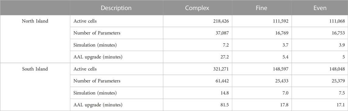
TABLE 1. List of characteristics resulting from the layering approach and parameterization for each model, including simulation times and times for parameter upgrades using automatic adaptive localization (AAL).

The open-source python package FloPy 3.3.5 (Bakker et al., 2021) was used to construct most of the MODFLOW input files. The Surface Water Network tool (SWN; Toews and Hemmings, 2019) was used to generate inputs for the Streamflow Routing Package (SFR2; Niswonger and Prudic, 2005) in MODFLOW. The PstFrom class (White et al., 2021) in the python package pyEMU (White et al., 2016) was used to ensure a consistent approach to representing adjustable parameters, observations, and predictions between the various models (see “Parameterization” section below and Supplementary Material). Additional python package libraries including NumPy, Pandas, and SciPy were used to pre-process data and post-process model results.

3.2 Discretization

Each of the model vertical structures explored in this study represents the same subsurface domain (horizontal and vertical extents) with a horizontal discretization of 2 km (Figures 1, 2). The specific depth and thickness of each layer is dependent on the spatially distributed depth to hydrogeologic basement (DHGB) as described in Westerhoff et al. (2019) and the layering scheme (Figure 3). A minimum layer thickness of 10 m and a minimum model thickness of 50 m is enforced for all models. The bottom of the top layer in all models is nominally 10 m below the surface. Routines in the SWN package that ensure stream reach elevations progress downstream from high elevation to low elevation can result in stream bed elevation being significantly lower than surface elevation, especially in steep terrain. While this is reflective of the often deep incision of streams in many parts of Aotearoa/New Zealand, it may require that the bottom of the surface layer is shifted down to accommodate the stream. The top of the model is unchanged to honour the elevation data, resulting in a thicker upper layer where streams are deeply incised (Figure 3).

FIGURE 1

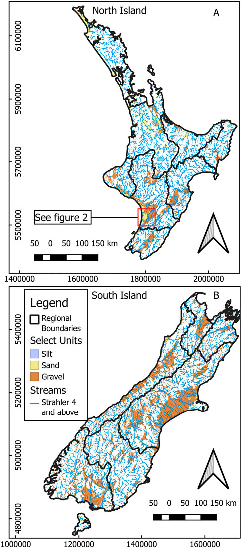
FIGURE 1. Map of the North Island (A) and South Island (B) of Aotearoa/New Zealand showing Strahler order four streams and above, regional boundaries, and hydrogeologic units of interest in this study (silt, sand, and gravel). Regional boundaries are used for manual localization in the IES method. Hydrogeologic units of interest are used to determine locations for history matching observations and predictions. See Figure 2 for a plan view of model specifics in the area shown by the red box.

FIGURE 2

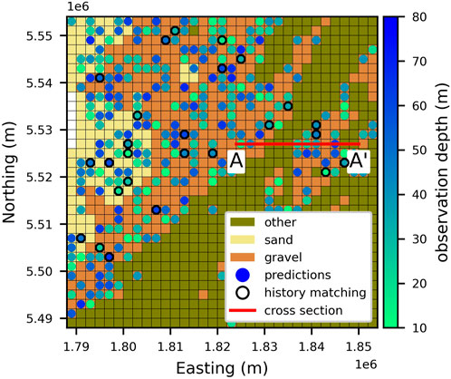
FIGURE 2. Detailed portion of the Aotearoa/New Zealand national groundwater model showing regional boundaries, hydrogeologic units, and observation locations (circles) used for history matching (black boarder) and predictions (no boarder). Observation depths are show by the colour bar. The red line (A,A′) shows the location of the cross section shown in Figure 3.

FIGURE 3

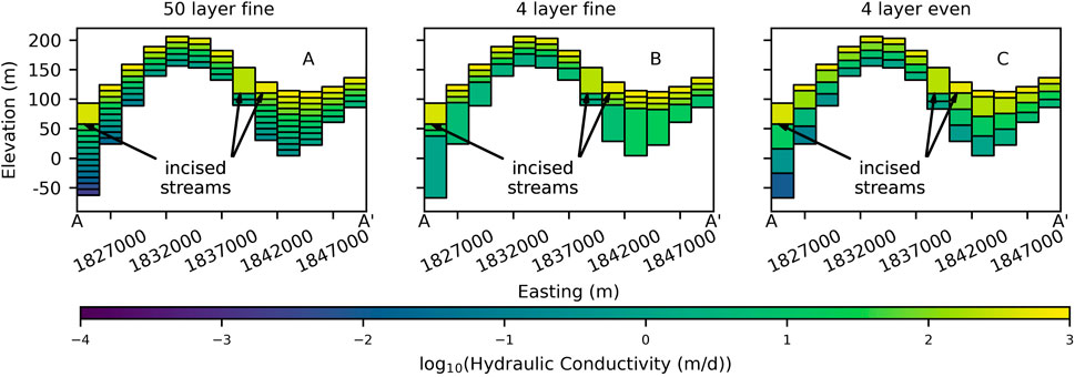
FIGURE 3. Cross-sections of A-A′ shown in Figure 2 illustrating discretization and upscaled hydraulic conductivity values (log(K)) for the (A) complex model, (B) fine model, (C) even model.

The vertical model structure with a constant vertical discretization of 10 m and up to 50 layers is used as the complex version of the system (Figure 3A; “complex” model). The actual number of layers depends on the depth of the model (DHGB) and any adjustments to the top layer needed to accommodate incised channels. Two additional layering approaches are investigated: 1) a four-layer model with three thin (nominally 10 m) upper layers and one deeper layer (Figure 3B; “fine” model), and 2) a four-layer model with three evenly distributed deeper layers (Figure 3C; “even” model).

3.3 Boundary conditions

Surface water sources in our models are either distributed recharge along the top surface of the model representing rainfall recharge or losing streams. In this study we use the Streamflow Routing Package (SFR2) which provides a more realistic and flexible way to simulate streamflow than other packages. For example, in the RIV package cells with a river boundary condition essentially act as a general head boundary when the groundwater head falls below the bottom of the streambed. This can lead to higher groundwater recharge compared to SFR2 (e.g., Foglia et al., 2018), creating higher gradients near streams, and incorrect simulation of streams as sources. The input data for the SFR2 package is generated for Strahler order four and above streams contained in the River Environment Classification database from the National Institute of Water and Atmospheric Research (National Institute of Water and Atmospheric Research, 2019) using the Surface Water Network (SWN) tool developed by the Institute of Geological and Nuclear Sciences (GNS; Toews and Hemmings, 2019).

Spatially distributed recharge from the nationwide model of groundwater recharge for Aotearoa/New Zealand (NGRM; Westerhoff et al., 2018) is added to the model using the RCHA package. The NGRM model considers the effects of precipitation, evapotranspiration, vegetation, topography, soils, and geology on groundwater recharge. However, overland flow due to saturation from below (i.e., Dunnian flow) is not considered in the NGRM model because the groundwater flow system is not well represented. Dunnian flow is simulated in our models by applying a head dependent flux boundary condition to the upper surface of the model using the drain package (DRN) and routing groundwater discharge to the surface or rejected recharge in cells where groundwater reaches the surface to the nearest SFR segment using the mover package (MVR). This also prevents unrealistically high groundwater heads in areas of high recharge and low conductivity. The general head boundary package (GHB) is used to represent the edge of the active model domain at the coast. See the MODFLOW documentation (Langevin et al., 2021) for a detailed description of these packages.

3.4 Age simulations

Locations of history matching targets and predictions (i.e., weighted and unweighted observations, respectively) in this study are limited to areas mapped as sand or gravel in the model, the materials that make up the most extensive and productive aquifers in Aotearoa/New Zealand (White P. A. et al., 2019). To avoid potential boundary effects, coastal boundary cells were excluded from the observation dataset. A total of 6,970 locations mapped as sand or gravel are randomly selected as observation locations: 2,056 for the North Island and 4,914 for the South Island, reflecting the relative abundance of sand and gravel aquifers on each island (Figure 1). The distribution of observations also reflects the relative abundance of these aquifer materials within each region. The mean depth of each observation is selected from a random distribution between the bottom of the top layer and either 80 m below the surface or 10 m above the bottom of the model, whichever is shallower. Observation locations were limited to 10 m above the bottom of the model to avoid potential stagnant conditions along the bottom of the model. The distribution of observation locations per layer for each model is listed in Supplementary Material. Each observation point is populated with 100 particles evenly distributed along the surface of a cylinder with a radius of 10 m and a height of 2 m. Particles are tracked from the observation location to the source, as determined by the steady-state flow field and the IFACE parameter in MODPATH (Pollock, 2012; see below).

Mean age is calculated from the travel times of particles originating from each location described above. The IFACE parameter in MODPATH specifies which cell face is considered the source for each boundary cell. For upper boundary cells in the RCH package the IFACE parameter is set to six indicating the source (i.e., zero age) is at the top of the cell. Abrams et al. (2013) showed that travel times to weak sink streams in a simple 1-layer model can be accurately simulated if the bottom of the stream channel is aligned with the top of the model and IFACE is set to 6 (i.e., the top face of the cell). However, in the current models where a stream may be incised hundreds of meters below the surface elevation, using the top of an SFR cell as the source can result in ages over 100 years higher than if the bottom of the cell is used (i.e., 0.5 m below the stream bed). Therefore, we set the IFACE parameter to 0 for all cells with SFR segment, indicating the source (i.e., zero age) is along the face of the boundary cell that is first intersected by the particle path during the backward particle tracking simulation.

3.5 Parameterization

The prior values of horizontal hydraulic conductivity (Kh), vertical hydraulic conductivity (K33), streambed hydraulic conductivity (Ksb), drain conductance (Cd), GHB conductance (Cghb), and porosity (ɸ) for all models are assigned consistently based on the main rock type in QMAP (GNS Science, 2012) and representative values found in the literature. The surface geology is assumed to extend to the DHGB (Westerhoff et al., 2019), except for units mapped as silt. Silt deposits are assumed to be 10 m thick and overly gravels with thickness determined by adjacent deposits. The hydraulic conductivity and porosity of the gravels overlain by silt is reduced by 10%. The hydraulic conductivity and porosity of all materials decrease as an exponential function of depth following Westerhoff et al. (2018).

Uncertainty for all parameters is addressed using parameter multipliers over four spatial scales (two scales geostatisical interpolation, zone multipliers, and layer multipliers; see Supplementary Material). Model inputs are the product of the multipliers and the “native” values. The initial value of all multipliers is one. The limits of each multiplier are reported in Table 2. The large range in parameter values accommodates: 1) the potential for inaccuracies in the mapping QMAP hydrofacies to the model grid, 2) the large uncertainty in hydraulic conductivity values for geologic materials (e.g., Domenico and Schwartz, 1998), and 3) the potential for parameters taking on physically unrealistic values to accommodate structural defects in the model, including due to averaging properties to accommodate different discretization approaches. Further details of model parameterization can be found in the Supplementary Material.

TABLE 2

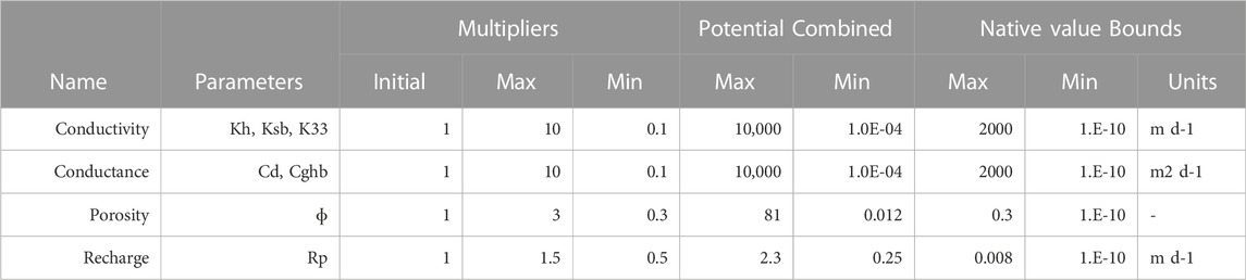
TABLE 2. Values of multiplier parameters, potential for combined multipliers, and native value bounds enforced for each parameter group.

The PstFrom utility in the pyEMU package is used to create the interface and input files for the PEST++ suite and generate the initial parameter ensemble. The parameter ranges are used to define a wide prior parameter distribution, representing ±3σ. The PstFrom.draw() method in pyEMU is used to draw an ensemble of stochastic parameter vectors (realizations) assuming multi-variate Gaussian distributions. We limit parameter values to physically realistic and numerically stable values by enforcing an “ultimate” upper and lower bound for “native” parameter values via the PstFrom utility (Table 2).

3.6 History matching

Simulated ages from a single stochastic realization of the complex model is used to define a set of observations representing the target values (i.e., “truth”). This dataset is free from real-world complication such as measurement noise and transience. Since the data were generated by the complex model, the complex model is endowed with precisely the appropriate parameter complexity to reproduce the results. This end-member case is compared to the simplified models to isolate the impacts of coarse vertical discretization. History matching to this data using the complex model shows how small ensembles can bias predictions, despite using a structurally perfect model.

A random sample of approximately 10% of the observations on each island are assigned a weight of one during the history matching process (204 out of 2,056 for the North Island, 504 out of 4,914 for the South Island). The other 90% (1,852 and 4,410, respectively) are retained as predictions with zero weights. This allows us to evaluate the implications of model simplification and the associated parameterization on model predictions following history matching. The number observations used for history matching in each layer of each model is listed in Supplementary Material.

The IES method, as implemented in the PEST++ suite, is used for history matching (White 2018; White et al., 2020; Welter et al., 2015). The IES method uses an empirical Jacobian matrix calculated using cross-covariances between ensembles of stochastic realizations of parameter vectors and simulated equivalents of historical observations constituting the history matching dataset. Too few realizations in the ensemble, compared to the span of the observations which determine the dimensions of the solution space, can cause spurious correlations. These spurious correlations for infeasible or impossible parameter-observation relationships can be “zeroed out” using localization (see below). The history matching process in IES can be further improved by using more realizations than the dimensionality of the calibration solution space to increase the rank of the empirical Jacobian.

Methods exist for estimating the dimensionality of the solution space using a high-fidelity, perturbation-based Jacobian (e.g., Doherty and Hunt, 2009). However, we are not aware of a similar method for estimating the solution space using an empirical Jacobian. Practitioners typically use ensembles of 50–150 realizations for parameter estimation. Hunt et al. (2021) use 300 realizations for a parameter estimation problem with 1,777 adjustable parameters and a diverse set of approximately 30,000 history matching targets to “ensure the solution space was fully represented and results were free from adverse effects of ensemble collapse.” Here we test the effects of using ensembles of 50, 100, 150, 200, and 300 realizations for history matching to a relatively simple dataset using each of the three model variations.

By default, PEST++ identifies prior data conflict (PDC) for weighted observation when the ensemble of observation values plus noise does not cover the ensemble of simulated values using the prior parameter ensemble. Observations with PDC are likely to cause bias as the history matching process seeks extreme parameter values to satisfy those observations. In this study, we retain observations with PDC in order to explore the potential impact on model predictions.

3.7 Localization

Localization masks spurious correlations between parameters and observations that can result from the use of a low-order ensemble. In this study, localization is initially based on groups defined by the 16 regions in Aotearoa/New Zealand, the boundaries of which typically follow major watershed boundaries. This groupwise localization scheme breaks correlations established between parameters in one region and observations in another. Zone and layer multiplier parameters are not included in this level of localization, meaning observations on a given island can influence zone and layer multipliers anywhere on that island. This groupwise localisation is very efficiently defined and implemented within PEST++ (White et al., 2021).

Localization also has the effect of increasing the rank of the empirical Jacobian used in the IES scheme, beyond that set by the size of the ensemble. Hence localization can mitigate the effects of truncation of the solution space if the ensemble size is too small. An alternative and automated localisation scheme can also be implemented in PEST++ using “automatic adaptive localization” (AAL; Luo, et al., 2018; White et al., 2021). AAL attempts to identify and mask spurious parameter-observation correlations generated by the stochastic nature of the ensembles for every parameter and observation pair. This process of localization results in a highly disjointed Jacobian matrix requiring numerous “local” parameter upgrade solves, which can become numerically expensive (Table 1). We explore the effectiveness of AAL using the lowest order ensemble (50 realizations).

4 Results

4.1 Mean phi

In general, model to measurement fits, as summarised by the mean objective function (phi or the L2-norm), decrease rapidly within the first three iterations (Figure 4). All three model vertical discretisation approaches display significant reductions in mean phi for all ensemble sizes, with all reducing to the same order of magnitude over six IES iterations. Generally, the simplified models of the North Island (Figures 4B, C) do not achieve the same reduction in phi as the complex model (Figure 4A) after six IES iterations. The simplified models of the South Island (Figures 4E, F) achieve similar values of mean phi as the complex model (Figure 4D) after six IES iterations. Interestingly the lower order ensembles often achieve the lowest values of mean phi for all models. Other than this, there is no apparent relationship between the rate of decrease and the level of model simplification or the size of the ensemble. Instead, the ensemble size and the number of iterations needed to attain a particular value of mean phi depends on the system being modelled (e.g., North Island vs. South Island) and the size of the ensemble. This seems particularly true for the structurally ‘perfect’ complex models (i.e., iteration 2 in Figure 4A and iterations 2 and 3 in 4D).

FIGURE 4

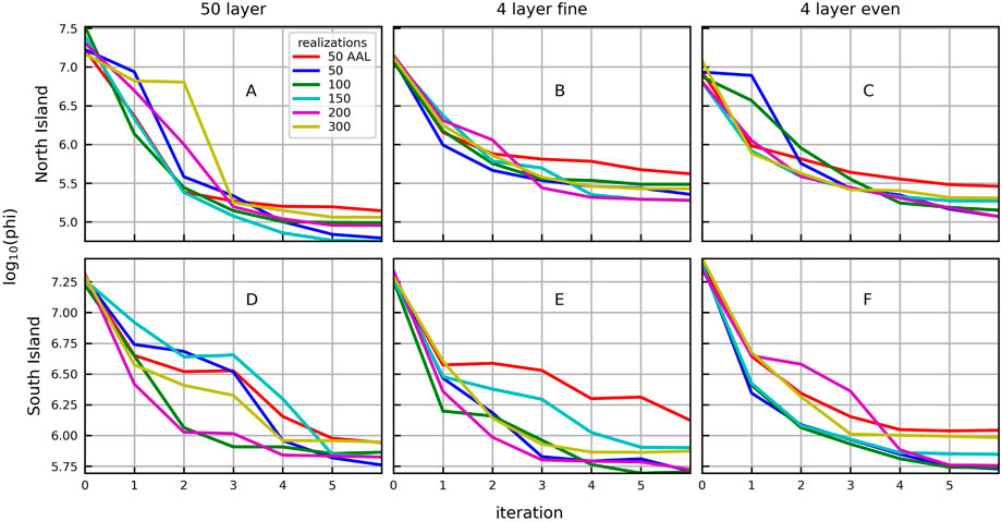
FIGURE 4. Plots of mean phi with iteration for the complex models (A,D), simplified fine models (B,E), and simplified even models (C,F) of the North Island (A–C) shown in Figure 3 (columns). Different ensemble sizes used in the IES history matching are shown by the colours.

The complex models contain the appropriate level of structural complexity and parameterization to adequately reproduce the calibration targets and predictions, since this 50-layer model was used to generate the ‘truth’ target observations using a single parameter vector chosen from the prior probability distribution. History matching using the complex models of the North Island results in a mean phi value that is lower than the simplified models after the third iteration, regardless of ensemble size (Figures 4A–C). However, this is not the case for the South Island. History matching of the South Island model using the 4-layer models produces mean phi values similar to, and occasionally lower than, the complex model after six iterations, depending on ensemble size (Figures 4D–F).

The ensembles with 50 realizations and AAL result in the highest mean phi (worst fit) after six iterations for all models. The ensemble with 300 realizations also results in a relatively high mean phi after six iterations for most of the models. Conversely, the ensemble with 50 realizations results in a relatively low mean phi after six iterations for most of the models.

4.2 History matching observations

The history matching targets are captured by the prior parameter ensemble for more than 92% of the weighted observation locations, for all ensemble sizes and all models (Pf < 8%; Figure 5 iteration 0). The complex model with 300 realizations performed the best in terms of history matching, with less than 0.5% failure for all iterations (Figures 5A, D). The highest prior failure (PDC) occurs with the 50-realization ensembles (2% < Pf < 8%; Figure 5, iteration 0), except for the complex model of the South Island (Pf = 0.2%; Figure 5D). The history matching process with 50 realizations and no AAL significantly increases the percentage of history matching observation locations for which the model fails to capture the truth (Pf >15%), except for the structurally perfect complex models.

FIGURE 5

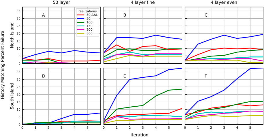
FIGURE 5. Percent failure (Pf) by iteration, ensemble size, and model structure for history matching targets (weighted observations) for the complex models (A,D), simplified fine models (B,E), and simplified even models (C,F) of the North Island (A–C) and South Island (D–F). Ensemble sizes are indicated by colours.

We can isolate the influence of structural errors from the history matching process by examining the percent failure at iteration 0 in Figure 5 for all model structures. This corresponds to prior data conflict (PDC) reported by PEST++. The PDC suggests structural defects in the fine model affect the North Island (Figure 5B) more than the even model (Figure 5C), while the opposite is true for the South Island (Figures 5E, 6F, respectively). The structural defects in the simplified models implied by the PDC are compounded through the history matching process, resulting in higher model failure rates with more iterations. This is particularly true using 50 realizations without AAL. The simplified models of the South Island with 50 realizations and no AAL have higher percentage of failure than the simplified models of the North Island for any given iteration, reaching 37.6% and 24.7% failure, respectively.

FIGURE 6

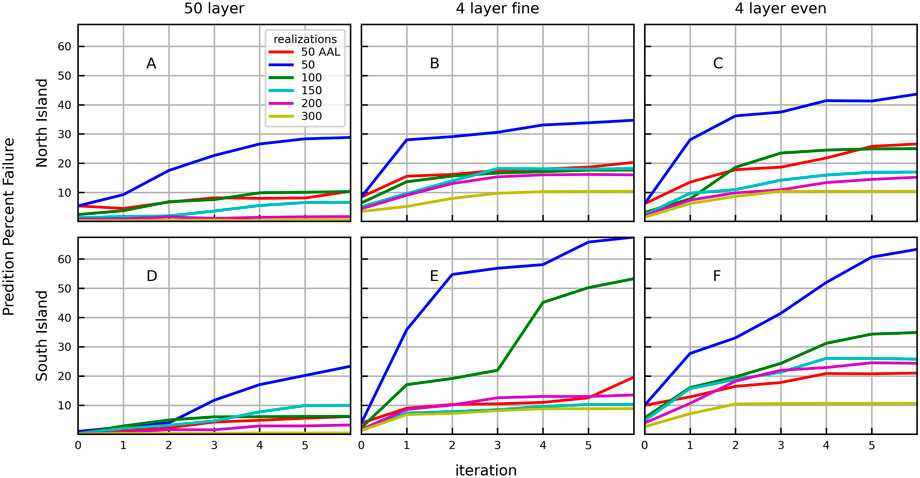
FIGURE 6. Percent failure (Pf) by iteration, ensemble size, and model structure for predictions (unweighted observations) for the complex models (A,D), simplified fine models (B,E), and simplified even models (C,F) of the North Island (A–C) and South Island (D–F). Ensemble sizes are indicated by colours.

The ability to capture the true value of the history matching dataset is improved with AAL. The failure rate of the predictions after six iterations using the structurally perfect complex models using 50 realizations with no AAL is 7.6% for the North Island and 8.6% for the South Island; this is reduced to 3.2% and 2.4%, respectively, using AAL.

4.3 Predictions

The predictions are captured by the prior parameter ensemble for more than 86% of the locations, for all ensemble sizes and all models (Pf < 14%; Figure 6 iteration 0). The complex model with 300 realizations performed the best in terms of prediction (Figures 6A, D), with less than 0.7% failure for all iterations, with no systematic change in prediction failure rates over iterations. The history matching process significantly increases prediction failure for all other models, particularly when using 50 realizations without AAL. Similar to the history matching targets, the simplified models of the South Island (Figures 6E, F) with 50 realizations and no AAL tend to have a higher percentage of failure for predictions than the North Island (Figures 6B, C), reaching 43.6% and 63.3%, respectively.

The ability to capture the true value of predictions is improved with AAL. The failure rate of the predictions after six iterations using the structurally perfect complex models and 50 realizations with no AAL is 28.8% for the North Island and 23.3% for the South Island; this is reduced to 10.4% and 6.1%, respectively, using AAL.

4.4 Parameter estimation: Prior and posterior distributions

The three model structures presented here support different levels of parameterization at depth, making it difficult to make direct comparisons of individual parameter adjustments for each model during the history matching process. However, for a single model structure we can examine how parameter ensembles of different sizes morph from prior to posterior through history matching in different ways.

Figure 7 provides an example of this for hydraulic conductivity multipliers from the complex (A) and fine (B) models of the South Island. After six iterations the history matching process with the complex model maintains a broad PDF using 300 realizations (Figure 7A yellow, 10-0.38–100.4) and 50 realizations with AAL (Figure 7A red, 10-0.12–100.28). These PDFs encompass the initial value of unity and hence still represent the initial value of hydraulic conductivity in native parameter space. However, using 50 realizations without AAL (Figure 7A solid blue) shows a narrower PDF that does not encompass the initial value of unity (100.11–100.24) despite achieving a lower value of phi. The posterior PDF does still fall within the prior PDF (Figure 7A, blue with stipples).

FIGURE 7

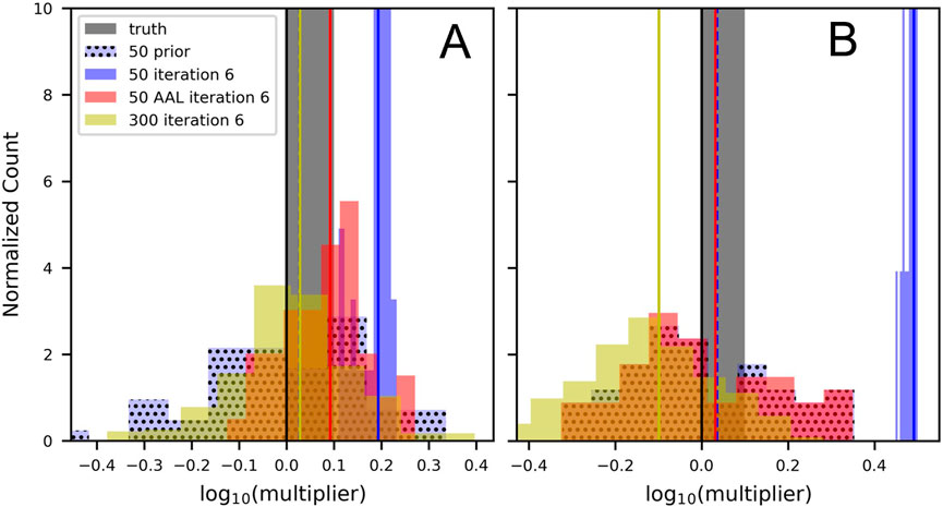
FIGURE 7. Probability density functions for hydraulic conductivity multipliers for the (A) complex model and (B) fine model of the South Island. The prior PDF for 50 realizations is shown in light blue with stipples. The mean of the posterior PDF for 50 realizations (blue), 50 realizations with AAL (red), and 300 realizations (yellow) ensembles are shown by vertical lines.

After six iterations the history matching process with the fine model shows similar behaviour using 300 realizations and 50 realizations with AAL (Figure 7B). However, the even the structurally complex model with a small ensemble without AAL shows a much narrower PDF that falls outside the prior PDF. This example illustrates how small parameter ensembles can result in collapse of the posterior parameter PDF. It also demonstrates the role of large ensembles and localization to prevent ensemble collapse. Figure 7 also shows how structural defects can corrupt the posterior PDF as parameters take on surrogate roles that accommodate for the missing parameters as model output to measurement matches are sought.

5 Discussion and conclusions

The numerical experiments described in this paper focus on the predictive performance implications of adopting structurally simple models and history matching with reduced ensemble sizes. The implications of the results of these experiments are considered in a decision support modelling context that relies on groundwater age simulations at a national scale. For this specific decision support context, we adopted a similar paired complex and simple model approach as documented in Doherty and Christensen (2011), Knowling et al. (2019), White et al. (2019a) and others. This method assesses the performance of simpler model structures in relation to a complex model structure. In synthetic experiments such as are documented in this paper, this complex model structure can represent the nominal “truth”, for the purposes of the study.

5.1 Model to measurement fits and predictive performance

On the basis of model to measurement fits, as summarised by the mean objective function (phi), one might consider in some cases that the simplified models is as effective as the complex model for simulating the system, e.g., the South Island simplified models examples. At first glance it may also appear that low realisation numbers are more than sufficient for conditioning parameters to system observations. However, the higher prediction failure rates (Pf) of the simplified models are not consistent with how well the model was able to fit the data (as reflected by the associated mean phi values). Many of the configurations that produce the best fits, or lowest mean phi, also produce the highest prediction failure rate.

The implications of good fits being a poor indicator of good predictive performance are not well understood in the larger modelling community. The demonstration of this issue in this paper is consistent with the recent discussions in Hunt et al. (2021) and Doherty and Moore (2021) in a numerical physically based modelling context, and Ruidas et al. (2021) in a data-driven modelling context. The interplay of predictive performance with model structural errors and ensemble size is discussed below.

5.2 Model structural errors and predictive performance

The predictive failure results relating to the 4-layer models conflate structural deficiencies with those arising from inadequate ensemble size. However, because the 300-realisation ensemble can be inferred to span the solution space (Hunt et al., 2021; Doherty and Moore 2019), the predictive impact from structural deficiencies can be isolated when exploring the 300-realisation ensemble results. Prediction failure occurs because the simplified (coarse) vertical discretization inhibits the ability of the model to represent the hydraulic property heterogeneity that occurs with depth; this heterogeneity places controls on groundwater flow paths and hence groundwater age. This simpler structure therefore compromises the ability of the model to process information from the history matching observations to the model parameters in a way that adequately informs the predictions, as evidenced by the higher prediction failure rate of the simplified models compared to the complex model.

The predictive performance of simplified models and smaller ensemble sizes is problem specific, as illustrated by differences in the geological contexts of the two models; the North and South Island models. In general, the South Island has more extensive and deeper gravel aquifers than the North Island. As such, parameters in the simplified models of the South Island represent parameters lumped over a greater depth interval. We observe that the greater the extent of parameter lumping (or upscaling), the greater structural related prediction errors will be, wherever predictions are sensitive to the hydraulic property detail that has been obscured by the lumping process.

5.3 Ensemble size, number of history matching iterations and predictive performance

History matching using smaller ensembles (particularly those without AAL) significantly increases failure for both history matching targets (phi) and predictions (Pf). This is evident for all versions of vertical model structures examined. These results again emphasise that good model to measurement fits are an insufficient criterion for predictive model efficacy, as described above.

The results also show that there is an increase in model predictive failure rate through history matching iterations for all discretisation versions, and across all ensemble sizes, except for the complex models with the 300 realizations ensemble, which remains below 1% over all iterations. This trend is especially evident in the simplified models and where the ensemble size is small. The 300-realization ensembles consistently provide the minimum predictive failure trend in all models, reaching a fairly constant value of 10% in the simplified models after the first few iterations. This indicates that the history matching process involving simpler models and/or inadequately sized ensembles, is forcing parameters to take on surrogate roles that can lead to parameter and predictive bias (Doherty and Moore 2019; Knowling et al., 2019).

This becomes clearer when examining the complex model with 300 realizations, for which we can assume that there is no structural model error, as the structure is the same as the ‘truth model’. For this complex model, because history matching does not appear to incur any increase in predictive failure, we can also assume that the 300 realizations sufficiently span the solution space. Therefore, the history matching and predictive ability of the complex model presented is compromised only by rank deficient Jacobian matrices associated with smaller ensembles. This effectively allows us to isolate the impact of deficiencies in model structure from those resulting from the history matching implementation with a rank deficient Jacobian. These rank deficiency related errors result from the smaller ensembles and hence insufficient dimensions in parameter space to realistically convey predictive error, i.e., some parameter combinations that the observations and predictions are sensitive to are not well represented in the smaller ensembles.

Localisation methods can address this to varying extents by increasing the rank of the Jacobian matrices. The automatic adaptive localization (AAL) was demonstrated to reduce model failure, which becomes more extreme with smaller ensembles. This is as it should be as AAL provides a method for mitigating the impacts of adopting small ensembles to some extent, which is a compromise that is often made when model run times are larger as discussed in Chen and Oliver 2017. This mitigation is achieved by removing spurious correlations from the parameter update calculations. It is this process that helps to guard against failure to capture the true values of both history matching targets and predictions. However, it should be noted that using AAL can incur a significant computational cost due to the potentially disjointed Jacobian.

5.4 Implications for design of large-scale groundwater age models

Results in this study suggest simplified layering schemes appropriate for large, national scale models may produce adequate results, provided large enough ensembles are used. However, history matching with simplified models and small ensembles is likely to produce unacceptably high failure rates. Acceptable model simplifications and adequate ensemble size is problem specific, as illustrated by the difference between the North and South Island models. This study suggests a reasonable combination of model simplification and ensemble size may be identified by a stable failure rate of weighted observations with iteration, as seen with the 300-realization ensemble for all models presented. In contrast, increasing failure rate of weighted observations with iteration, as seen in the lower order ensembles and simplified models, suggests a concomitant increase in prediction failure rate.

Finally, we note that while other national groundwater models exist (Döll and Fiedler, 2008; De Lange et al., 2014), the development of a national groundwater age model, which to the authors knowledge is a world first in terms of scale, represents an extensive modelling effort. This type of development includes the running of numerous numerical experiments as part of the model design process, one of which is documented in this paper. The number of moving parts is enormous, and the cognitive load of a modeller is limited, and hence we believe that this effort would likely not be possible without adopting a scripted modelling workflow that spans task ranging from model discretization to highly parameterized inversion (Leaf and Fienen 2022). This workflow benefits enormously from the existence of opensource software packages and the community that contributes to their development and maintenance (Bakker et al., 2021; White et al., 2016; White et al., 2021).

Data availability statement

The raw data supporting the conclusions of this article will be made available by the authors, without undue reservation.

Author contributions

WK is responsible for the model construction and analysis of results. CM and WK are responsible for the experimental design. CM and BH provided important theoretical and practical input throughout the experiment. All authors contributed to the writing of this manuscript.

Funding

This work was funded by the New Zealand Ministry of Business Innovation and Employment (Grant No. C05X1803) and was also supported by GNS Science Groundwater Strategic Science Investment Fund (SSIF).

Acknowledgments

The authors would like to thank all those who support, develop, and contribute to the ecosystem of opensource software and tools that made this research possible.

Conflict of interest

The authors declare that the research was conducted in the absence of any commercial or financial relationships that could be construed as a potential conflict of interest.

Publisher’s note

All claims expressed in this article are solely those of the authors and do not necessarily represent those of their affiliated organizations, or those of the publisher, the editors and the reviewers. Any product that may be evaluated in this article, or claim that may be made by its manufacturer, is not guaranteed or endorsed by the publisher.

Supplementary material

The Supplementary Material for this article can be found online at: https://www.frontiersin.org/articles/10.3389/feart.2022.972305/full#supplementary-material

References

Abrams, D., Haitjema, H., and Kauffman, L. (2013). On modeling weak sinks in MODPATH. Groundwater 51 (4), 597–602.

PubMed Abstract | CrossRef Full Text | Google Scholar

Bakker, M., Post, V., Hughes, J. D., Langevin, C. D., White, J. T., Leaf, A. T., et al. (2021). FloPy v3.3.5 — release candidate. U.S. Geological Survey Software Release. doi:10.5066/F7BK19FH

CrossRef Full Text | Google Scholar

Chen, Y., and Oliver, D. S. (2013). Levenberg–Marquardt forms of the iterative ensemble smoother for efficient history matching and uncertainty quantificationcient history-matching and uncertainty quantification. Comput. Geosci. 17 (4), 689–703. doi:10.1007/s10596-013-9351-5

CrossRef Full Text | Google Scholar

Chen, Y., and Oliver, D. S. (2017). Localization and regularization for iterative ensemble smoothers. Comput. Geosci. 21, 13–30. doi:10.1007/s10596-016-9599-7

CrossRef Full Text | Google Scholar

De Lange, W. J., Prinsen, G. F., Hoogewoud, J. C., Veldhuizen, A. A., Verkaik, J., Essink, G. H. P. O., et al. (2014). An operational, multi-scale, multi-model system for consensus-based, integrated water management and policy analysis: The Netherlands hydrological instrument. Environ. Model. Softw. 59, 98–108. doi:10.1016/j.envsoft.2014.05.009

CrossRef Full Text | Google Scholar

Doherty, J., and Christensen, S. (2011). Use of paired simple and complex models to reduce predictive bias and quantify uncertainty. Water Resour. Res. 47 (12), 12534. doi:10.1029/2011WR010763

CrossRef Full Text | Google Scholar

Doherty, J. E. (2015). PEST and its utility support software, Theory. Watermark Numerical Publ.

Google Scholar

Doherty, J., and Hunt, R. J. (2009). Two statistics for evaluating parameter identifiability and error reduction. J. Hydrology 366 (1-4), 119–127. doi:10.1016/j.jhydrol.2008.12.018

CrossRef Full Text | Google Scholar

Doherty, J., and Moore, C. R. (2019). Decision support modeling: Data assimilation, uncertainty quantification, and strategic abstraction. Groundwater 58, 327–337. doi:10.1111/gwat.12969

PubMed Abstract | CrossRef Full Text | Google Scholar

Doherty, J., and Moore, C. R. (2021). Decision-support modelling viewed through the lens of model complexity. Available at: https://gmdsi.org/blog/monograph-decision-support-modelling-viewed-through-the-lens-of-model-complexity/.

Google Scholar

Doherty, J., and Welter, D. (2010). A short exploration of structural noise. Water Resour. Res. 46. doi:10.1029/2009WR008377

CrossRef Full Text | Google Scholar

Döll, P., and Fiedler, K. (2008). Global-scale modeling of groundwater recharge. Hydrol. Earth Syst. Sci. 12, 863–885. doi:10.5194/hess-12-863-2008

CrossRef Full Text | Google Scholar

Domenico, P. A., and Schwartz, F. W. (1998). Physical and chemical hydrogeology, 506. New York: Wiley.

Google Scholar

Foglia, L., Neumann, J., Tolley, D. G., Orlo_, S. G., Snyder, R. L., and Harter, T. (2018). Modeling guides Groundwater management in a basin with river–aquifer interactions. Calif. Agric. (Berkeley). 72, 84–95. doi:10.3733/ca.2018a0011

CrossRef Full Text | Google Scholar

GNS Science (2012). Qmap. Available at: https://www.gns.cri.nz/Home/Our-Science/Land-and-Marine-Geoscience/Regional-Geology/Geological-Maps/1-250-000-Geological-Map-of-New-Zealand-QMAP (accessed on January 3, 2017).

Google Scholar

Gosses, M., and Wöhling, T. (2019). Simplification error analysis for groundwater predictions with reduced order models. Adv. Water Resour. 125, 41–56. doi:10.1016/j.advwatres.2019.01.006

CrossRef Full Text | Google Scholar

Guppy, L., Uyttendaele, P., Villholth, K. G., and Smakhtin, V. (2018). Groundwater and sustainable development goals: Analysis of interlinkages. UNU-INWEH report series, issue 04. Hamilton, Canada: United Nations University Institute for Water, Environment and Health.

Google Scholar

Guthke, A. (2017). Defensible model complexity: A call for data-based and goal-oriented model choice. Groundwater 55 (5), 646–650. doi:10.1111/gwat.12554

PubMed Abstract | CrossRef Full Text | Google Scholar

Hunt, R. J., Fienen, M. N., and White, J. T. (2020). Revisiting ‘an exercise in groundwater model calibration and prediction’ after 30 Years: Insights and New directions. Groundwater 58, 168–182. doi:10.1111/gwat.12907

PubMed Abstract | CrossRef Full Text | Google Scholar

Hunt, R. J., White, J. T., Duncan, L. L., Haugh, C. J., and Doherty, J. (2021). Evaluating lower computational burden approaches for calibration of large environmental models. Groundwater 59, 788–798. doi:10.1111/gwat.13106

PubMed Abstract | CrossRef Full Text | Google Scholar

Jakeman, A. J., Barreteau, O., Hunt, R. J., Rinaudo, J., Ross, A., Arshad, M., and Hamilton, S. (2016). “Integrated groundwater management: An overview of concepts and challenges,” in Integrated groundwater management: Concepts, approaches and challenges. A. J. Jakeman, O. Barreteau, R. J. Huntet al. (Cham: Springer International Publishing), 3–20.

CrossRef Full Text | Google Scholar

Jaydhar, A. K., Pal, S. C., Saha, A., Islam, A. R. M. T., and Ruidas, D. (2022). Hydrogeochemical evaluation and corresponding health risk from elevated arsenic and fluoride contamination in recurrent coastal multi-aquifers of eastern India. J. Clean. Prod. 369, 133150. doi:10.1016/j.jclepro.2022.133150

CrossRef Full Text | Google Scholar

Knowling, M. J., White, J. T., Moore, C. R., Rakowski, P., and Hayley, K. (2020). On the assimilation of environmental tracer observations for model-based decision support. Hydrol. Earth Syst. Sci. 24, 1677–1689. doi:10.5194/hess-24-1677-2020

CrossRef Full Text | Google Scholar

Knowling, M. J., White, J. T., and Moore, C. R. (2019). Role of model parameterization in risk-based decision support: An empirical exploration. Adv. Water Resour. 128, 59–73. doi:10.1016/j.advwatres.2019.04.010

CrossRef Full Text | Google Scholar

Langevin, C. D., Hughes, J. D., Banta, E. R., Provost, A. M., Niswonger, R. G., and Panday, S. (2021). MODFLOW 6 modular hydrologic model version 6.2.2. U.S. Geological Survey Software Release. doi:10.5066/F76Q1VQV

CrossRef Full Text | Google Scholar

Leaf, A. T., and Fienen, M. N. (2022). Modflow-setup: Robust automation of groundwater model construction. Front. Earth Sci. (Lausanne). 10. doi:10.3389/feart.2022.903965

CrossRef Full Text | Google Scholar

Luo, X., Bhakta, T., and Naevdal, G. (2018). Correlation-based adaptive localization with applications to ensemble-based 4d seismic history-matching. SPE J. 23, 396–427. doi:10.2118/185936-pa

CrossRef Full Text | Google Scholar

McMahon, P. B., Plummer, L. N., Bohlke, J. K., Shapiro, S. D., and Hinkle, S. R. (2011). A comparison of recharge rates in aquifers of the United States based on groundwater-age data. Hydrogeol. J. 19, 779–800. doi:10.1007/s10040-011-0722-5

CrossRef Full Text | Google Scholar

Ministry for the Environment (2020). National policy statement for freshwater management. Available from https://environment.govt.nz/publications/national-policy-statement-for-freshwater-management-2020 (accessed Jan 13, 2022).

Google Scholar

Ministry for the Environment, , and Stats, N. Z. (2021). New Zealand’s environmental reporting series: Our land 2021. Available from www.stats.govt.nz (accessed June 13, 2022).

Google Scholar

Morgenstern, U., Daughney, C. J., Leonard, G., Gordon, D., Donath, F. M., and Reeves, R. (2015). Using groundwater age and hydrochemistry to understand sources and dynamics of nutrient contamination through the catchment into Lake Rotorua, New Zealand. Hydrol. Earth Syst. Sci. 19, 803–822. doi:10.5194/hess-19-803-2015

CrossRef Full Text | Google Scholar

National Institute of Water and Atmospheric Research (2019). freshwater-and-estuaries/management-tools/river-environment-classification. Available from https://niwa.co.nz/freshwater-and-estuaries/management-tools/river-environment-classification-0 (accessed May 29, 2019).

Google Scholar

Niswonger, R. G., and Prudic, D. E. (2005). Documentation of the streamflow-routing (SFR2) package to include unsaturated flow beneath streams—a modification to SFR1. U.S. Geol. Surv. 50.

Google Scholar

Pollock, D. W. (2012). User guide for MODPATH version 6—a particle-tracking model for MODFLOW: U.S. Geol. Surv. Tech. Methods 6–A41, 58.

PubMed Abstract | Google Scholar

Rajanayaka, C., Donaggio, J., and McEwan, H. (2010). Update of water allocation data and estimate of actual water use of consented takes 2009-10. Ministry for theEnrivornment.

Google Scholar

Regan, R. S., Juracek, K. E., Hay, L. E., Markstrom, S. L., Viger, R. J., Driscoll, J. M., et al. (2019). The US Geological Survey National Hydrologic Model infrastructure: Rationale, description, and application of a watershed-scale model for the conterminous United States. Environ. Model. Softw. 111, 192–203.

CrossRef Full Text | Google Scholar

Ruidas, D., Pal, S. C., Islam, A. R. M. T., and Saha, A. (2021). Characterization of groundwater potential zones in water-scarce hardrock regions using data driven model. Environ. Earth Sci. 80, 809. doi:10.1007/s12665-021-10116-8

CrossRef Full Text | Google Scholar

Sanford, W. E. (2011). Calibration of models using groundwater age. Hydrogeol. J. 19, 13–16. doi:10.1007/s10040-010-0637-6

CrossRef Full Text | Google Scholar

Siebert, S., Burke, J., Faures, J. M., Frenken, K., Hoogeveen, J., Döll, P., et al. (2010). Groundwater use for irrigation – A global inventory. Hydrol. Earth Syst. Sci. 14, 1863–1880. doi:10.5194/hess-14-1863-2010

CrossRef Full Text | Google Scholar

Singh, A. (2014). Groundwater resources management through the applications of simulation modeling: A review. Sci. total Environ. v499, 414–423. doi:10.1016/j.scitotenv.2014.05.048

PubMed Abstract | CrossRef Full Text | Google Scholar

Stauffer, F., Guadagnini, A., Butler, A., Franssen, H. H., Wiel, N., Bakr, M., et al. (2005). Delineation of source protection zones using statistical methods. Water Resour. manage. 19, 163–185. doi:10.1007/s11269-005-3182-7

CrossRef Full Text | Google Scholar

Toews, M. W., and Hemmings, B. (2019). “A surface water network method for generalising streams and rapid groundwater model development,” in New Zealand Hydrological Society Conference, Rotorua, 3-6 December 2019, 166–169.

Google Scholar

Watson, T. A., Doherty, J. E., and Christensen, S. (2013). Parameter and predictive outcomes of model simplification. Water Resour. Res. 49 (7), 3952–3977. doi:10.1002/wrcr.20145

CrossRef Full Text | Google Scholar

Welter, D. E., White, J. T., Doherty, J. E., and Hunt, R. J. (2015). “PEST++ version 3, a parameter estimation and uncertainty analysis software suite optimized for large environmental models,” in U.S. Geological Survey Techniques and Methods Report 7–C12, 54.

Google Scholar

Westerhoff, R., Rawlinson, J., and Tschritter, C. (2019). New Zealand groundwater atlas: Depth to hydrogeological basement. Lower hutt (NZ). GNS Sci. 19

Google Scholar

Westerhoff, R., White, P., and Rawlinson, Z. (2018). Incorporation of satellite data and uncertainty in a nationwide groundwater recharge model in New Zealand. Remote Sens. 10 (1), 58. doi:10.3390/rs10010058

CrossRef Full Text | Google Scholar

White, J. T., Hemmings, B., Fienen, M. N., and Knowling, M. J. (2021). Towards improved environmental modeling outcomes: Enabling low-cost access to high-dimensional, geostatistical-based decision-support analyses. Environ. Model. Softw. 139, 105022. doi:10.1016/j.envsoft.2021.105022

CrossRef Full Text | Google Scholar

White, J. T. (2018). A model-independent iterative ensemble smoother for efficient history-matching and uncertainty quantification in very high dimensions. Environ. Model. Softw. 109, 191–201. doi:10.1016/j.envsoft.2018.06.009

CrossRef Full Text | Google Scholar

White, J. T., Doherty, J. E., and Hughes, J. D. (2014). Quantifying the predictive consequences of model error with linear subspace analysis. Water Resour. Res. 50 (2), 1152–1173. doi:10.1002/2013wr014767

CrossRef Full Text | Google Scholar

White, J. T., Fienen, M. N., and Doherty, J. E. (2016). A python framework for environmental model uncertainty analysis. Environ. Model. Softw. 85, 217–228. doi:10.1016/j.envsoft.2016.08.017

CrossRef Full Text | Google Scholar

White, J. T. (2017). Forecast first: An argument for groundwater modeling in reverse. Groundwater 55, 660–664. doi:10.1111/gwat.12558

PubMed Abstract | CrossRef Full Text | Google Scholar

White, J. T., Knowling, M. J., and Moore, C. R. (2019a). Consequences of groundwater-model vertical discretization in risk-based decision-making. Ground Water 58, 695–709. doi:10.1111/gwat.12957

PubMed Abstract | CrossRef Full Text | Google Scholar

White, P. A. (2001). “Groundwater resources in New Zealand,” in Groundwaters of New Zealand. Editors M. R. Rosen, and P. A. White (Wellington: New Zealand Hydrological Society), 45–75.

Google Scholar

White, P. A., Moreau, M., Mourot, F., and Rawlinson, Z. J. (2019b). New Zealand groundwater atlas:hydrogeological-unit map of New Zealand. Lower Hutt (NZ): GNS Science, 88.

Google Scholar

Wildemeersch, S., Goderniaux, P., Orban, Ph., Brouyére, S., and Dassargues, A. (2014). Assessing the effects of spatial discretization on large-scale flow model performance and prediction uncertainty. J. Hydrology 510, 10–25. doi:10.1016/j.jhydrol.2013.12.020

CrossRef Full Text | Google Scholar