A geothermal heat flow model of Africa based on random forest regression

1 Introduction

Temperature gradients measured directly from boreholes are sparsely available. Estimates of continental geothermal heat flow (GHF) can, therefore, only be derived indirectly from geophysical and geological quantities such as geomagnetic, seismic, gravity, topographic, and compositional data. This holds in particular for recent studies of Antarctica [e.g. (Burton-Johnson et al., 2020; Lösing and Ebbing, 2021; Stål et al., 2021)] but also for Africa, where advanced methods are required to incorporate sparse direct measurements with such indirect observables. Studies by (Shahdi et al., 2021; He et al., 2022) compared several machine learning (ML) methods for geothermal heat flow modeling at regional scales and indicated that these methods can perform as good as, and sometimes better than, physics-based models. Physics-based models [such as, e.g. (Lösing et al., 2020; Sobh et al., 2021)] often require various simplifications and are feasible only for few geophysical observables. Thus, if one wants to include several different geophysical and geological observables for the prediction of GHF, as seems necessary for continental-scale models, purely physics-based models become unfeasible. Data-driven machine learning approaches for Greenland and Antarctica, both with very sparse direct GHF information, have been presented, e.g., in (Rezvanbehbahani et al., 2017; Lösing and Ebbing, 2021; Stål et al., 2021), with the former two publications using gradient boosted regression trees and the latter one a similarity detection approach. A random forest approach for modeling marine heat flow has been investigated in (Li et al., 2022).

In this paper, we follow such a random forest approach to generate a GHF model for Africa, initially based on sixteen different geophysical and geological observables. However, due to an intrinsic importance ranking of the random forest approach, we reduce the number of used observables to eleven for the final GHF model (namely, the used observables are Moho depth, lithospheric density, LAB depth, geoid, free air and Bouguer anomaly, topography, S wave velocity, shape index, Curie temperature depth and P wave velocity). This final model coincides well with already existing regional geothermal heat flow information. A more detailed evaluation and interpretation can be found in Section 4.

2 Data and geological background

2.1 Geothermal heat flow data

The New Global Heat Flow (NGHF) is a compilation of previous GHF databases containing 69,730 data points, with an average continental GHF of about 67 mWm⁻² (Lucazeau, 2019). The NGHF rates the quality of the measurements as follows: A, B, C, D, and Z. To filter training data, we extract records with A and B ratings that correspond to less than 10% and less than 20% variation of GHF measurement in boreholes, respectively. As a result, the number of records is reduced to 12,707, with minimum and maximum values of -3.0 and 5,146.0 mWm⁻², respectively, and a mean of 66.1 mWm⁻². Furthermore, we exclude records from NGHF with missing spatial coordinates and missing GHF values. Additionally, we exclude records at high latitudes beyond -60° and 80°, respectively, and oceanic records (deeper than 1,000 m below sea level).

Exploratory data analysis revealed the presence of 63 measurements with GHF values (>200 mWm⁻²) and 13 measurements with GHF values (<10 mWm⁻²) inside the A labeled data and 115 measurement points (>200 mWm⁻²) and 36 measurement points (<10 mWm⁻²) inside the A and B labeled data. Supplementary Figure S2 in the supplementary material depicts the locations of those measurements. These values, together with negative values, are questionable and could be attributed either to some local thermal activities such as hydrothermal circulation or errors in measurements (Bachu, 1988). Hence, we exclude these values for our further continental-scale evaluations. As a result, we obtain a final dataset containing both A and B ratings. This GHF data will serve as our reference throughout the course of this paper. Additionally, we generate a reference dataset containing only A labeled data. Results for the latter data set can be found in Supplementary Figure S5 in the supplementary material and are briefly discussed in Section 4.1. The GHF model presented in the main body of the paper is based on reference data labeled A and B.

Figure 1 shows density plots and the basic statistics of the eventually used data. It also depicts the histogram of binned GHF measurements in Africa involving all records, records after removal of questionable and incomplete information, records after removal of deep-sea information, and records based on different quality ratings n the NGHF database. Additionally, Supplementary Figure S1 describes the same information regarding global GHF measurements.

FIGURE 1

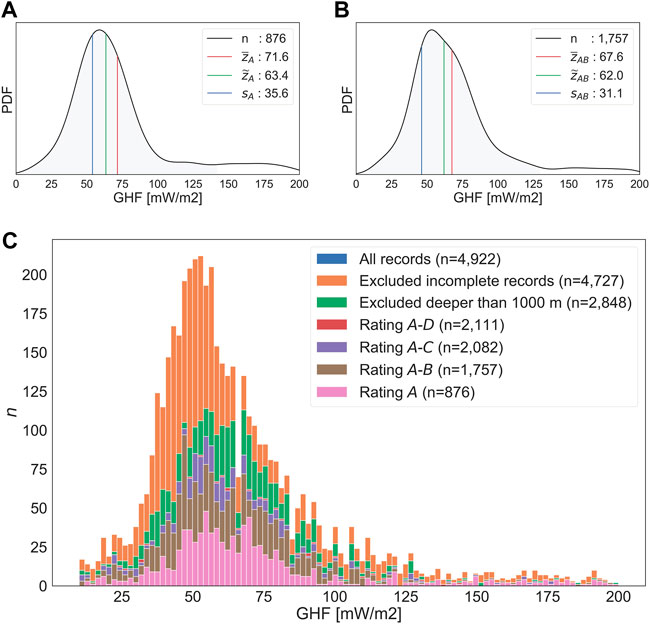
FIGURE 1. (A) Density plot of GHF measurements in Africa labeled A without questionable values (B) Density plot of GHF measurements in Africa labeled A and B without questionable values, (C) Histogram of binned GHF measurements in Africa involving all records, records after removal of questionable and incomplete information, records after removal of deep-sea information, and records based on different quality ratings in the NGHF database. (Lucazeau, 2019). $\bar{z}$ = mean, $\tilde{z}$ = median, s = standard deviation.

2.2 Geological and geophysical observables

We chose sixteen further geological and geophysical observables for the GHF model prediction, including global as well as regional datasets for Africa (see Table 1). They are of mixed types, categorical and continuous. Crossplots between these observables and the available GHF reference data from Section 2.1 are shown in Figure 2.

TABLE 1

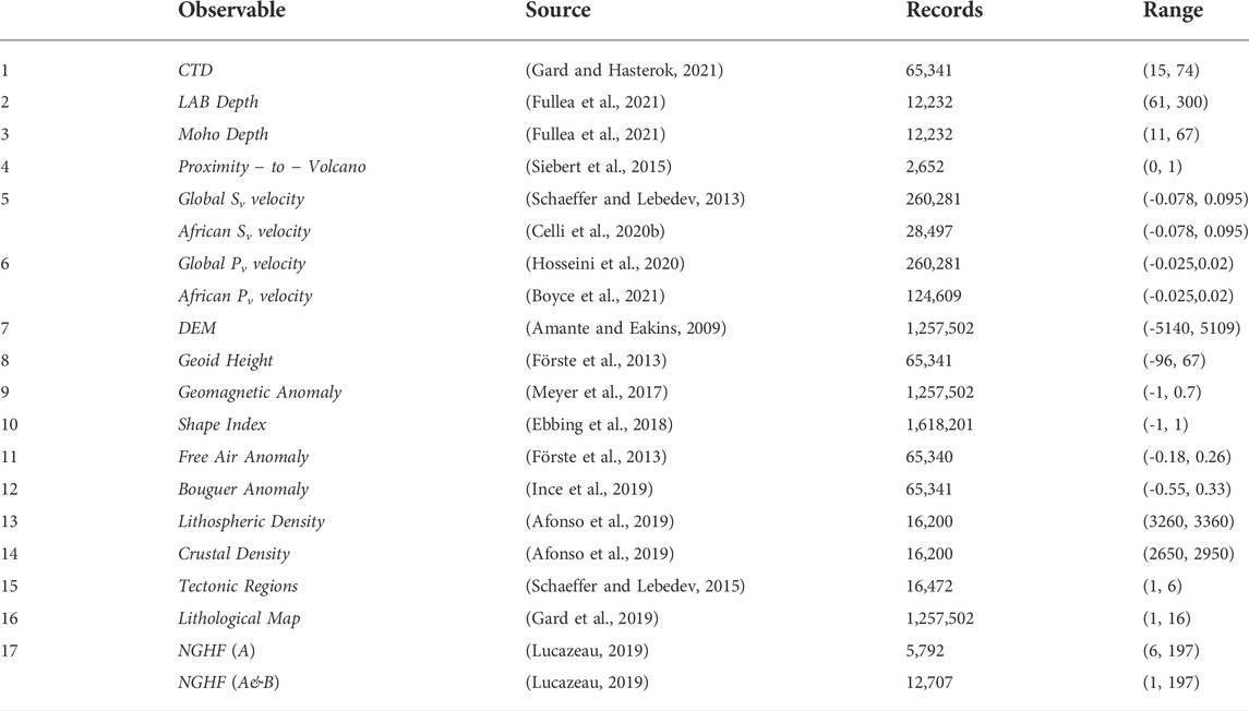
TABLE 1. The observables used in this study with their sources, number of records and range.

FIGURE 2

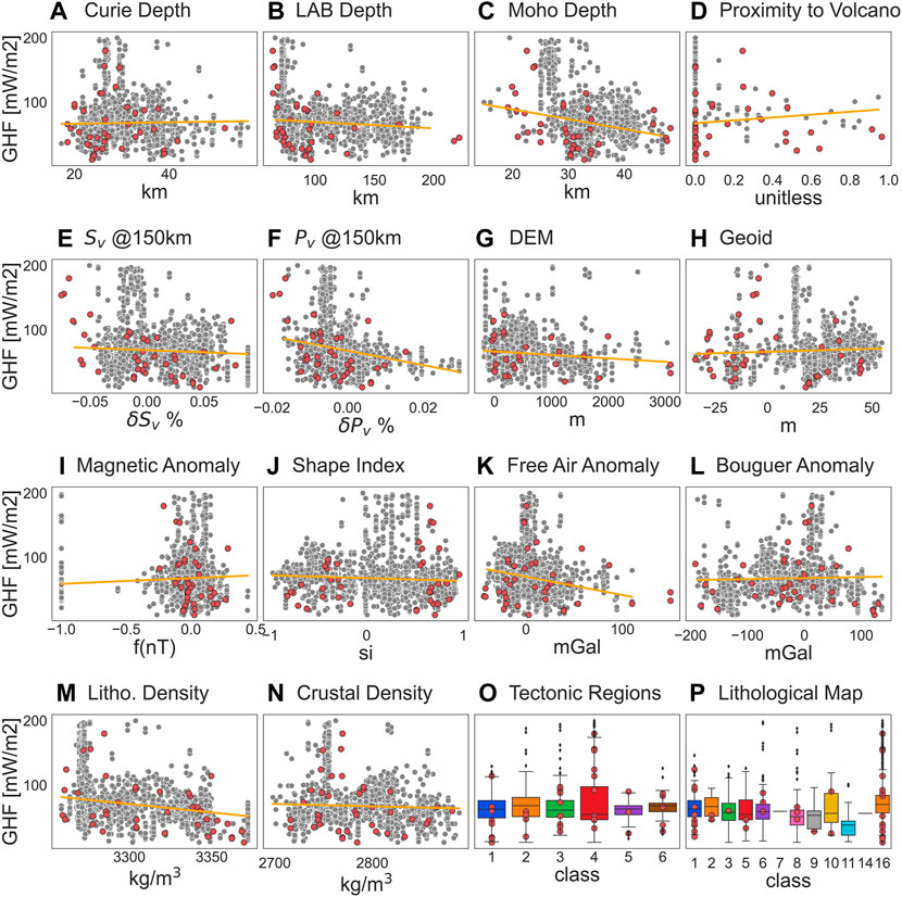
FIGURE 2. Cross plots of the GHF measurements against geological and geophysical observables; the orange lines indicate the linear regression results. Categorical observables are illustrated by boxplots. Red dots indicate outliers. Classes for tectonic regionalizations refer to: 1 = Cratons; 2 = Precambrian Fold Belts and Modified Cratons; 3 = Phanerozoic Continents; 4 = Ridges & Backarcs; 5 = Oceanic; 6 = Oldest Oceanic. Classes for GLIM inside Africa refer to: 1 = Unconsolidated sediments; 2 = Siliciclastic sedimentary rocks; 3 = Pyroclastics; 5 = Carbonate sedimentary rocks; 6 = Evaporites; 7 = Acid volcanic rocks; 8 = Intermediate volcanic rocks; 9 = Basic volcanic rocks; 10 = Acid plutonic rocks; 11 = Intermediate plutonic rocks; 14 = Water Bodies; 16 = No Data.

Curie temperature depth (CTD) is obtained from the global model of (Gard and Hasterok, 2021). Moho and LAB depths are provided by the WINTERC-G global model from (Fullea et al., 2021). Upper mantle velocity models may shed light on the mantle and lithospheric components of the GHF (Shapiro and Ritzwoller, 2004). S wave velocities are derived from the global model SL 2013sv, and the African regional model AF2019 is obtained from (Schaeffer and Lebedev, 2013) and (Celli et al., 2020b), respectively. The P wave velocity global model, DETOX-P1, and the African regional model, AFRP20, are obtained from (Hosseini et al., 2020) and (Boyce et al., 2021). In our set of observables, we consider the P and S wave velocities at a depth of 150 km. The Digital Elevation Model (DEM), which represents the topography in m, is obtained from ETOPO1 (Amante and Eakins, 2009). ETOPO1 is a global relief model of the earth’s surface with 1-arcminute resolution. We used the EMAG2v3 geomagnetic anomaly map in nT from (Meyer et al., 2017). EMAG2v3 is a global grid of geomagnetic anomalies compiled from satellite, shipboard, and airborne magnetic measurements at 2-arcminute resolution. Due to the variation of geomagnetic anomaly data over several orders of magnitude, we transformed it via M_log = sgn(M) ln (1 + M/400) and clipped it to the interval [ − 1, 1], where M is the original geomagnetic anomaly data and M_log the transformed quantity that we use in the course of this paper. The four observables that reflect gravity information are derived from the EIGEN-6C4 global model (Förste et al., 2013). Calculations of the geoid in m, free-air gravity, and Bouguer gravity in mGals are performed by ICGEM (Ince et al., 2019). We also include the gravity field curvature shape index (Ebbing et al., 2018) derived from the two horizontal and independent components of the satellite gravity gradient from GOCE data (Pail et al., 2010). This is a dimensionless quantity with an interval of [ − 1, 1]. The average densities of the crust and lithosphere in kg/m⁻³ are obtained from the LithoRef18 (Afonso et al., 2019) global model.

The proximity to the nearest young volcano is calculated from the Global Volcanism Program (Siebert et al., 2015). The distances between our target locations and a specific volcano are computed along great circles and this distance is then transformed into proximity via 1 − (dist/100) and clipped to a unitless range of [0, 1]. Volcanoes farther away than 100 km from the specific target location are excluded. We also included categorical data on lithologies and tectonic regions. The global lithology map (GLiM) database was compiled by (Gard et al., 2019). It groups the surface lithologies into sixteen classes. As for the tectonic regionalization, the model proposed by (Schaeffer and Lebedev, 2015) delineates six tectonic regions.

We choose the IsolationForest routine (Liu et al., 2008; Buitinck et al., 2013) to detect outliers in the data described above. Those removed outliers are depicted as red points in Figure 2. The Pearson correlation matrix for the given observables before and after deleting the outliers is provided in Supplementary Figures S3 and S4 in the supplementary material. Figure 3 illustrates those eleven observables (among the original sixteen observables) that have eventually been used for the generation of the GHF model presented in this paper. These observables are Moho depth, lithospheric density, LAB depth, geoid, free air and Bouguer anomaly, topography, S wave velocity, shape index, Curie temperature depth and P wave velocity. The remaining observables have been neglected due to an importance ranking described later on in Section 3.3.

FIGURE 3

FIGURE 3. Illustration of the observables used in this study (A) Measured GHF, (B) Moho depth, (C) Lithospheric average density, (D) Lithosphere–Asthenosphere Boundary (LAB) depth, (E) Geoid, (F) Free air gravity anomaly, (G) Bouguer anomaly, (H) Digital Elevation Model (DEM), (I) S_v velocity, (J) Shape index, (K) Curie temperature depth, (L) P_v velocity.

2.3 Gridding of the data

We imported the previously described observables and stacked them into a multi-dimensional grid of 0.5° × 0.5° resolution using Xarray (Hoyer et al., 2016). In grid cells where no data for the geological or geophysical observable under consideration is available or where the resolution of the original data is not sufficient, we interpolate via inverse distance weighting (IDW) if the observable is of continuous type. The samples of the GHF data described in Section 2.1 are not interpolated but simply reassigned to the grid cells nearest to the sample locations. In the course of the paper, we refer to the samples at grid cells where GHF data is available as reference data (including GHF as well as all further geological and geophysical observables). All samples at grid cells where no GHF information is available are denoted as target data (including all geological and geophysical observables other than GHF). These are the locations at which we want to predict GHF values.

2.4 Geological background of africa

The African continent is composed mainly of Precambrian terranes, assembled in the Late Neoproterozoic-Early Paleozoic Pan-African orogeny (Begg et al., 2009). Confer Figure 4 for an illustration. Three major cratons identified in Africa are the West African, Congo and Kalahari Cratons, with the smaller Tanzanian Craton located east of Congo, and Saharan Metacraton at the North (Sobh et al., 2020)). The greater Kalahari Craton consists of Kaapvaal and Zimbabwe cratons separated by the Limpopo Belt (de Wit et al., 1992) and the Rehoboth basin (Muller et al., 2009) to the west. The Congo Craton in central Africa hosts three Archean shield areas, parts of which are probably covered by the Congo basin: the Gabon-Cameroon (GC) in the Northwest, Kasai block (KB) in the central East, and Angolan craton (AC) along the western border south of the Gabon Cameroon (Celli et al., 2020a).

FIGURE 4

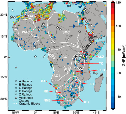
FIGURE 4. Simplified tectonic map of Africa with Cratons, Cratonic blocks, and other relevant tectonic units. Cratons are plotted in white polygons, KA = Kalahari Craton; CC = Congo Craton; WAC = West African Craton; SMC = Saharan Metacraton. Cratonic blocks: BB = Bangweulu Block; ZC = Zimbabwe Craton; TC = Tanzanian Craton; KC = Kaapvaal Craton; AC = Angola Craton; KB = Kasai Block; GC = Gabon–Cameroon Block. RB = Rehoboth Block; NNB = Namaqua-Natal Belt; ASZ = Aswa Shear Zone. Symbols of circle, triangle, square, diamond and hexagon represent the Reference GHF with A, B, C, D, and Z ratings respectively, derived from the global compilation of GHF database (Lucazeau, 2019). White asterisks = distribution of Volcanoes.

Toward Northern Africa, the West African Craton (WAC) and the Saharan Metacraton (SMC) are separated by the West African Mobile Zone (WAMZ). In the Cenozoic, widespread volcanism affected the African continent, mainly related to Pan-African crustal reactivation (Ashwal and Burke, 1989), continental rifting (Thorpe and Smith, 1974), hotspots (e.g., Hoggar, Tibesti, Darfur and Cameroon Volcanic Line), and the East African Rift System (EARS). The EARS is a seismically and volcanically active rift system (Sengör and Burke, 1978), whose geodynamic origin is under debate. Some studies support the origin of EARS as plume origin; Afar plume (Ebinger et al., 1989) or multiple plumes (Rogers et al., 2000) or even connected to the African Superplume (Hansen and Nyblade, 2013). The EARS is formed of Eastern and Western Branches. The Eastern Branch is a volcanic reach system consisting of Afar and Main Ethiopian Rifts. The Western Branch is younger with less volcanic activity (Ebinger et al., 1989).

3 Methodology

3.1 Random forest regression

A random forest (RF) is a collection of T decision trees, with each tree being able to provide a separate GHF prediction for the set of target observables $\mathcal{T}$. Each tree within the forest is built from a subset of the available reference observables $\mathcal{R}$, where each subset contains information on at most P randomly chosen observables (among the sixteen available observables). Furthermore, by D we denote the maximum possible depth of each tree, by S the minimum number of samples required in a leaf node of a tree, and by K the required minimum number of samples in an internal node of a tree in order to allow a further split this node. We call h = (T, P, D, S, K) the hyperparameters of the random forest. Once a RF is built for a certain set of hyperparameters, the predicted GHF value is obtained by averaging over the separate predictions of all T decision trees. The GHF model obtained this way will be denoted by AFQ. A detailed description of the concept of RF regression can be found in the original publication (Breiman, 2001).

3.2 Training the random forest

To clarify the procedure, we denote by $\mathcal{R}=\{(z_n^{\text{r}},{\mathbf{y}}_n^{\text{r}}):n=1,\dots ,N\}$ the set of reference observables ${\mathbf{y}}_n^{\text{r}}$ (cf. Section 2.2; each ${\mathbf{y}}_n^{\text{r}}$ contains sixteen entries covering the available observables) and corresponding reference GHF values $z_n^{\text{r}}$ (cf. Section 2.1; for our model we only use reference samples located within the African continent). The set of target observables is denoted by $\mathcal{T}=\{{\mathbf{y}}_m^{\text{t}}:m=1,\dots ,M\}$, comprising the observables described in Section 2.2 at locations where no GHF information is available. In order to train the RF, we use 90% of the samples for actually building the RF and the remaining 10% for cross-validation, resulting in N_cv samples for cross-validation (this procedure is iterated for ten different random choices of subsets). The optimal hyperparameters h are chosen by minimizing the mean square error (MSE)

$\mathrm{M}\mathrm{S}\mathrm{E}\left(\mathbf{h}\right)=\frac{1}{N_{\text{cv}}}\sum _{i=1}^{N_{\text{cv}}}{\left|z_i^{\text{r}}-{\widehat{z}}_{i,\mathbf{h}}^{\text{RF}}\right|}^2,(1)$

where $z_i^{\text{r}}$ denotes the available reference GHF in the cross-validation subset, and ${\widehat{z}}_{i,\mathbf{h}}^{\text{RF}}$ denotes the corresponding GHF predicted by the trained RF for the particular hyperparameters h. We simply test a range of 150 combinations of hyperparameters and, among them, choose the h with the minimum MSE(h). The eventual hyperparameters for our model are: T=450, P=6, D=20, S=2, and K=7. For the numerical implementation of this RF approach, we use the code provided by Sklearn (Buitinck et al., 2013) and Scikit-Optimize (Head et al., 2018). The initial GHF model then comprises the heat flow values ${\widehat{z}}_{m,\mathbf{h}}^{\text{RF}}$ predicted for the target observables ${\mathbf{y}}_m^{\text{t}}$ in $\mathcal{T}$, using the trained RF with optimized hyperparameters h.

3.3 Observable selection

Related decision tree-based methods have been used, e.g., in (Rezvanbehbahani et al., 2017; Lösing and Ebbing, 2021) for the prediction of GHF. However, in the gradient boosted setup used in these references, the trees are generated iteratively and require a regularization term to prevent overfitting while in the RF setup, the trees can be computed in parallel and overfitting is prevented by the random selection of observables for each tree and the eventual averaging of the predictions over all trees. What both methods have in common is that they can provide the user with an importance ranking of the involved observables. The importance is based on measuring the reduction of variance within a single decision tree due to that particular observable (the higher the reduction of variance, the more important is the observable; the importance is subsequently normalized to a relative importance with values in the interval [0, 1]). The importance of the observable for the entire RF is obtained by averaging over the importances for all trees.

The ranking due to the importance criterion from above is indicated by the green bars in Figure 5A. At this point, we want to mention that the ranking procedure turned out to be very sensitive to the choice of training data (e.g., only including GHF values up to 160 mW/m² in the training process for the RF significantly changed the ranking compared to including values up to 200 mW/m², as we have done for our final model). Figure 5A reveals that the proximity to volcano has hardly any importance. This seems counterintuitive, considering that proximity to volcano had fairly high importance in other studies [e.g., in Lösing and Ebbing (2021)]. This deviation may be explained by the sparsity of this observable in our dataset for Africa. However, we do not want to overinterpret the explanatory power of the importance ranking, but we rather use it as an orientation for the selection of a subset of observables for our final GHF model.

FIGURE 5

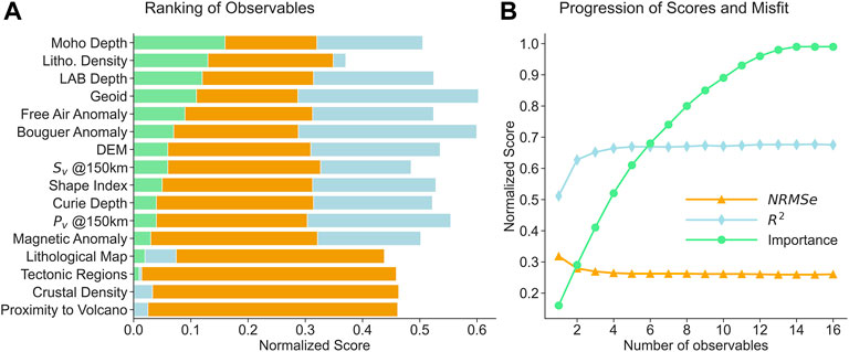
FIGURE 5. (A) Relative importance of the observables, coefficient of determination R², and normalized root mean square error NRMSe ranked by their contribution to the RF prediction, (B) Same scores as in the left figure but in a cumulative sense for the entire RF model based on different numbers of observables.

Using the ranking from above, we have recursively built several GHF models based on an increasing number of observables. The normalized root mean square error (NRMSe) and the coefficient of determination (R²) for each model are indicated in Figure 5B. It can be seen that both scores do not improve significantly when including more than the four most important observables. However, since we want to give some weight to the importance ranking, we opted to include eleven observables (i.e., Moho depth, lithospheric density, LAB depth, geoid, free air and Bouguer anomaly, topography, S wave velocity, shape index, Curie temperature depth and P wave velocity) to have a cumulative importance higher than 90%. In Supplementary Figure S6 of the supplementary material, GHF models for different numbers of observables and their residuals to the final model based on eleven observables are indicated. In fact, these residuals show that four observables do not suffice to capture all GHF structures while using all sixteen observables only leads to minor differences to the model based on eleven observables. Therefore, the latter model is the one discussed here in more detail (cf. Section 4).

3.4 Model uncertainty

As described before in Section 3.3, in the main body of the paper, we only present the GHF model built from the eleven most important observables. However, we use all obtained GHF models based on reference GHF data labeled A and B (including those shown in the supplementary material; altogether this amounts to twelve models) to compute the quantity

$\mathrm{r}\mathrm{a}\mathrm{n}\left(x_m^{\text{t}}\right)=\frac{{\max }_i{\mathrm{A}\mathrm{F}\mathrm{Q}}^i\left(x_m^{\text{t}}\right)-{\min }_i{\mathrm{A}\mathrm{F}\mathrm{Q}}^i\left(x_m^{\text{t}}\right)}{2},(2)$

which captures the range among these models at the target location $x_m^{\text{t}}$ (by AFQⁱ we denote the model based on the i most important observables according to the ranking in Figure 5). This property should not be considered a statistically proper definition of uncertainty, but it captures the variations due to the number of included observables. However, it does not include variations due to noise in the data (this has been tried to be reduced by a proper data selection) nor due to sampling bias (i.e., an insufficient representation of the geology at the target location by the training data). The latter is briefly discussed in Section 4.1 when comparing GHF models trained with data labeled A and B and models trained only with data labeled A.

As a final say, we want to mention that the RF approach used here, as well as the machine learning approaches used in other publications mentioned throughout this paper, are solely based on similarity structures between the geological and geophysical observables at a single location. They do not reflect spatial correlations of the observables.

4 Results and discussion

We present the modeled GHF together with the associated uncertainties. Additionally, we provide an evaluation of the modeled GHF and its geological implications.

4.1 The GHF model over africa

Figure 6 shows the predicted GHF for Africa based on a random forest trained with the eleven most important observables (according to the importance ranking from Figure 5) and GHF reference data labeled A and B. We name this model AFQ. A visualization of the same model without overlain details can be consulted in Supplementary Figure S7, Supplementary Figures S5 and S6 in the supporting material show various alternative versions of AFQ, trained with reference data containing samples labeled A and B as well as with reference data containing only samples labeled A. Comparing the models trained solely with GHF data labeled A to those trained with data labeled A and B, it becomes obvious that the models only trained with A labeled data do not capture the high GHF zone in Algeria (which is covered mostly by B labeled reference data). This underlines the expectation that the capability of generalization of the trained RF strongly depends on the training data, the so-called sampling bias. In this case, it would suggest that the geological and geophysical situation in Algeria is different from the areas where A labeled GHF data is available. For the sake of completeness, Supplementary Figure S8 in the supplementary material also shows the predictions of AFQ for the oceanic areas surrounding Africa and for the Arabian peninsula, although we do not provide a more detailed interpretation here.

FIGURE 6

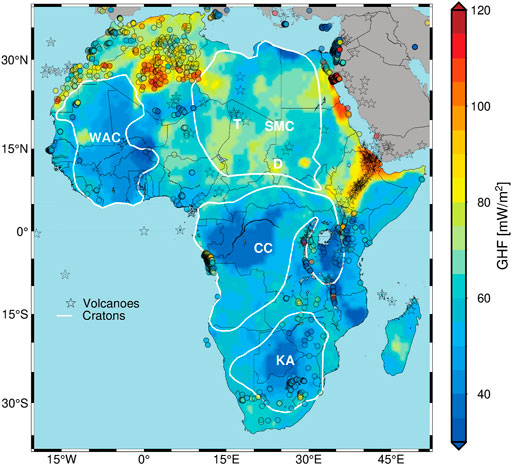
FIGURE 6. Modeled GHF of Africa based on eleven observables (AFQ), overlain with the locations of the reference GHF data. White polygons represent the major cratonic units in Africa, D = Darfur Dome; T = Tibesti Massif. Asterisks = distribution of Volcanoes.

4.2 Model evaluation

Figure 7A indicates that the agreement of AFQ with direct measurements is generally good with a NRMSe of 0.21. Also, the R² value of 0.79 indicates a good fit. On average, the AFQ model overestimates GHF values by 2.3%. Figure 7B shows the density plots of reference values and predicted values of AFQ. The model reveals a certain inability to predict high GHF values. Hence its standard deviation is lower than that of the reference GHF data. Also Figure 7A shows that for high values (>125 mWm⁻²) the model’s predictions become more unstable. This could be due to an underrepresentation of such high values in the training dataset, amounting to only 5.5% of the training data (i.e., 95 samples).

FIGURE 7

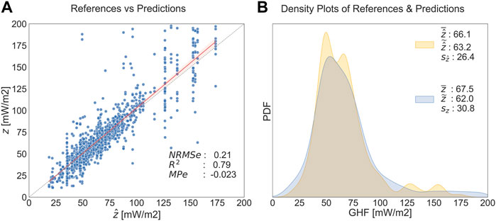
FIGURE 7. Performance indicators for the GHF model over Africa (AFQ) (A) Scatter plot of reference vs. predicted values together with coefficient of determination R², NRMSe and Mean Percentage error MPe; (B) Probability density plot of reference and predicted values. Light orange refers to predicted GHF values denoted by $\widehat{z}$, whereas light blue refers to measured GHF values denoted by z; $\bar{z}$ = mean, $\tilde{z}$ = median, s = standard deviation.

4.3 Model uncertainty

Figure 8A shows the quantity

$\mathrm{C}\mathrm{V}\left(x_m^{\text{t}}\right)=\frac{\left|\mathrm{A}\mathrm{F}\mathrm{Q}\left(x_m^{\text{t}}\right)-\overline{\mathrm{A}\mathrm{F}\mathrm{Q}}\right|}{\overline{\mathrm{A}\mathrm{F}\mathrm{Q}}},(3)$

similar to the common coefficient of variation at the target location $x_m^{\text{t}}$ (with $\overline{\mathrm{A}\mathrm{F}\mathrm{Q}}$ denoting the mean predicted heat flow over Africa and $\mathrm{A}\mathrm{F}\mathrm{Q}(x_m^{\text{t}})$ the predicted heat flow at location $x_m^{\text{t}}$). In regions without available reference GHF data, elevated CV values might indicate that AFQ actually “predicts” geothermal heat flow (based on the underlying trained random forest) and not just “averages” to a global mean. This is the case, e.g., in the Gabon craton, EARS, and northern Egypt. However, in contrast to this, there also exist various regions that are lacking reference GHF data and which reveal low CV values, i.e., the predicted value is close to the global mean. In those cases, it is difficult to distinguish if this is due to the lack of reference GHF information in these regions or if these values actually reflect valid geological information. Figure 5B shows the model variation based on the range (2) among GHF models trained with different numbers of observables. The predicted heat flow reveals high variations in eastern and northwestern parts of Africa. One can observe that these areas of increased variation correlate with areas lacking reference GHF information or areas covered mainly by reference values labeled B, e.g., in Algeria. They seem to be particularly affected by the choice of target observables.

FIGURE 8

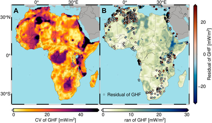
FIGURE 8. (A) Coefficient of variation for AFQ as defined by “CV” in (3), indicating the deviation of the predicted heat flow from the African mean; (B) Variation of predicted heat flow as defined by the quantity “ran” in (2), indicating the range of predicted heat flow values due to different numbers of observables used for training the random forest (a larger range means an increased variation among the different models). The residuals between reference GHF and the predicted values of AFQ (the final model trained with eleven observables) are overlaid as circles.

4.4 Interpretation

GHF is known to be broadly correlated with the tectonic setting of a region (Jaupart et al., 2007). The GHF model shown in Figure 6 indicates large-scale low-heat flow regions associated with the more stable tectonic regimes (e.g., KC; CC; and TC). Such results are highly consistent with the seismic tomographic results, showing high-velocity values in the upper mantle in these areas (Fishwick and Bastow (2011); Emry et al. (2019); Celli et al. (2020a)).

High GHF values are seen most clearly in the most active tectonics parts (e.g., EARS). Underneath the EARS, pronounced high-heat flow is modeled. EARS is considered as a remarkable geothermal potential in Africa due to geothermal sources related to magmatism and volcanism along the rift axis. There is much more variability in our model in the western branch compared to the eastern branch. In general, GHF values decrease away laterally from the EARS and EARS extends further south down to the Tanzanian Craton. Comparing geothermal heat flow with lithospheric thickness derived from seismic tomography is not straightforward and caution should be taken due to the effects of partial melting, attenuation, and rheology changes between asthenosphere and lithosphere. However, recent seismic tomography studies inferred a significant mantle velocity reduction of the S wave velocity in regions of Cenozoic volcanism due to thinning of the lithosphere (Fishwick and Bastow (2011); Emry et al. (2019); Celli et al. (2020a); Sobh et al. (2020)). Moderate to high GHF exists in northern Morocco, where GHF values partially exceed 100 mWm⁻². This is in agreement with the results of (Rimi, 2000). Similar high GHF values (>80 mWm⁻²) are present in a large area of western Algeria. Heat flow in this area has been previously modeled by (Lesquer and Vasseur, 1992). Along the West African Rift System (WARS) in the northeast of Nigeria, the modeled GHF values are >90 mWm⁻², which has been recorded also in (Kwaya et al., 2016). Beneath the Darfur hot spot, our model correctly predicts high GHFs. This is also the case along the Tibesti volcanic region, however, with lower values. Overall, our modeled heat flow values correlate with the lithospheric thickness, low heat flow is associated with cratonic blocks (e.g. CC), and high heat flow coincides with mobile belts and rifting areas (e.g, EARS), which is in good agreement with surface wave tomography estimates at global and continental scales (Fishwick and Bastow (2011); Emry et al. (2019); Celli et al. (2020a); Sobh et al. (2020). Consistent with how GHF relates to thin LAB, thin Moho, and low lithospheric density, an elevated GHF occurs in central Madagascar. In addition, an elevated GHF in western and southern Arabia agrees well with slow S and P wave velocity, high free air and high Bouguer anomalies, low lithospheric density, thin Moho, as well as thin CTD (confer Supplementary Figure S8 for a visualization of AFQ that includes the Arabian peninsula). Similarly, an increased heat flow in South Sudan shows correlations with LAB, CTD, lithospheric density, and seismic tomography. The estimates in these three spots clearly correlate with increased elevation relative to their surroundings. On the other hand, an increased heat flow occurs in southern Senegal that does not follow such patterns relating GHF to some of the observables. Furthermore, the model could not describe the actually known high GHF in the Hoggar area of Algeria.

A physics-based geothermal heat flow map of Southern Africa obtained from a single observable (namely, the Curie depth as inverted from magnetic anomaly information) has been presented in (Sobh et al., 2021). It is notable that the multi-observable based model AFQ presented here predicts lower heat flow along South African cratonic blocks (KC and ZC), while the model by (Sobh et al., 2021) exhibits very high heat flow regions, especially in the Kalahari Magnetic Lineament.

5 Conclusion

The objective of this paper is to present the geothermal heat flow model AFQ over continental Africa, based on RF regression. It tries to address the challenges encountered with direct GHF measurements in Africa, namely, sparsity, non-uniformity, and uncertainty. Due to this limitation, estimates of continental GHF are derived indirectly from various geophysical and geological quantities. Conventional ways to address these issues, e.g., by implementing physics-based models, require various simplifications and are feasible only for few geophysical observables. Therefore, approaches that allow for multiple observables, like RF regression, need to be explored. RF is a decision tree-based algorithm where overfitting is reduced by averaging the predicted values of each estimator within the generated ensemble. Due to an intrinsic importance ranking, AFQ trains with the eleven most important observables among sixteen available observables (i.e., Moho depth, lithospheric density, LAB depth, geoid, free air and Bouguer anomaly, topography, S wave velocity, shape index, Curie temperature depth and P wave velocity) at a resolution of 0.5° × 0.5°. The ability of the model to predict GHF values has been discussed and compared to several models trained with a different number of observables. In agreement with available geological and GHF information, AFQ shows elevated GHF around the red sea and along the east and west African rift systems, low GHF values around major cratons as well as cratonic blocks, and intermediate values elsewhere. For future work, it would be important to provide a more sophisticated quantification of uncertainty as well as to incorporate spatial correlation into random forest approaches as used here for GHF modeling.

Data availability statement

The original contributions presented in the study are included in the article/Supplementary Materials, the script and data generated in this study can be found here: https://zenodo.org/badge/latestdoi/494554790.

Author contributions

The authors confirm their contribution to the paper as follows: study conception, design, and data collection: MA-A; analysis and interpretation of results: MA-A, MS; revision and supervision: MS, CG. All authors reviewed the results and contributed to the draft and final version of the manuscript.

Acknowledgments

We thank the editor and two anonymous reviewers for their constructive criticism that helped to improve our manuscript. Also, this work has been partially funded by BMWi (Bundesministerium für Wirtschaft und Energie) within the joint project ‘SYSEXPL—Systematische Exploration’, grant ref. 03EE4002B, and Centre d’Etudes et de Recherche de Djibouti (CERD).

Conflict of interest

The authors declare that the research was conducted in the absence of any commercial or financial relationships that could be construed as a potential conflict of interest.

Publisher’s note

All claims expressed in this article are solely those of the authors and do not necessarily represent those of their affiliated organizations, or those of the publisher, the editors and the reviewers. Any product that may be evaluated in this article, or claim that may be made by its manufacturer, is not guaranteed or endorsed by the publisher.

Supplementary material

The Supplementary Material for this article can be found online at: https://www.frontiersin.org/articles/10.3389/feart.2022.981899/full#supplementary-material

References

Afonso, J. C., Salajegheh, F., Szwillus, W., Ebbing, J., and Gaina, C. (2019). A global reference model of the lithosphere and upper mantle from joint inversion and analysis of multiple data sets. Geophys. J. Int. 217, 1602–1628. doi:10.1093/gji/ggz094

CrossRef Full Text | Google Scholar

Amante, C., and Eakins, B. W. (2009). Etopo1 1 arc-minute global relief model: Procedures, data sources and analysis. noaa technical memorandum nesdis ngdc-24. Natl. Geophys. Data Cent., NOAA 10, V5C8276M. doi:10.1594/PANGAEA.104840

CrossRef Full Text | Google Scholar

Ashwal, L. D., and Burke, K. (1989). African lithospheric structure, volcanism, and topography. Earth Planet. Sci. Lett. 96, 8–14. doi:10.1016/0012-821x(89)90119-2

CrossRef Full Text | Google Scholar

Bachu, S. (1988). Analysis of heat transfer processes and geothermal pattern in the alberta basin, Canada. J. Geophys. Res. 93, 7767–7781. doi:10.1029/jb093ib07p07767

CrossRef Full Text | Google Scholar

Begg, G., Griffin, W., Natapov, L., O’Reilly, S. Y., Grand, S., O’Neill, C., et al. (2009). The lithospheric architecture of Africa: Seismic tomography, mantle petrology, and tectonic evolution. Geosphere 5, 23–50. doi:10.1130/ges00179.s2

CrossRef Full Text | Google Scholar

Boyce, A., Bastow, I., Cottaar, S., Kounoudis, R., Guilloud De Courbeville, J., Caunt, E., et al. (2021). Afrp20: New p-wavespeed model for the african mantle reveals two whole-mantle plumes below east Africa and neoproterozoic modification of the Tanzania craton. Geochem. Geophys. Geosyst. 22, e2020GC009302. doi:10.1029/2020GC009302

CrossRef Full Text | Google Scholar

Breiman, L. (2001). Random forests. Mach. Learn. 45, 5–32. doi:10.1023/a:1010933404324

CrossRef Full Text | Google Scholar

Buitinck, L., Louppe, G., Blondel, M., Pedregosa, F., Mueller, A., Grisel, O., et al. (2013). API design for machine learning software: Experiences from the scikit-learn project. ECML PKDD Workshop Lang. Data Min. Mach. Learn., 108–122. doi:10.48550/arXiv.1309.0238

CrossRef Full Text | Google Scholar

Burton-Johnson, A., Dziadek, R., and Martin, C. (2020). Review article: Geothermal heat flow in Antarctica: Current and future directions. Cryosphere 14, 3843–3873. doi:10.5194/tc-14-3843-2020

CrossRef Full Text | Google Scholar

Celli, N. L., Lebedev, S., Schaeffer, A. J., and Gaina, C. (2020a). African cratonic lithosphere carved by mantle plumes. Nat. Commun. 11, 92–10. doi:10.1038/s41467-019-13871-2

PubMed Abstract | CrossRef Full Text | Google Scholar

Celli, N. L., Lebedev, S., Schaeffer, A. J., Ravenna, M., and Gaina, C. (2020b). The upper mantle beneath the south atlantic ocean, south America and Africa from waveform tomography with massive data sets. Geophys. J. Int. 221, 178–204. doi:10.1093/gji/ggz574

CrossRef Full Text | Google Scholar

de Wit, M. J., Jones, M. G., and Buchanan, D. L. (1992). The geology and tectonic evolution of the pietersburg greenstone belt, South Africa. Precambrian Res. 55, 123–153. doi:10.1016/0301-9268(92)90019-k

CrossRef Full Text | Google Scholar

Ebbing, J., Haas, P., Ferraccioli, F., Pappa, F., Szwillus, W., and Bouman, J. (2018). Earth tectonics as seen by goce-enhanced satellite gravity gradient imaging. Sci. Rep. 8, 16356. doi:10.1038/s41598-018-34733-9

PubMed Abstract | CrossRef Full Text | Google Scholar

Ebinger, C., Bechtel, T., Forsyth, D., and Bowin, C. (1989). Effective elastic plate thickness beneath the east african and Afar plateaus and dynamic compensation of the uplifts. J. Geophys. Res. 94, 2883–2901. doi:10.1029/jb094ib03p02883

CrossRef Full Text | Google Scholar

Emry, E. L., Shen, Y., Nyblade, A. A., Flinders, A., and Bao, X. (2019). Upper mantle Earth structure in Africa from full-wave ambient noise tomography. Geochem. Geophys. Geosyst. 20, 120–147. doi:10.1029/2018gc007804

CrossRef Full Text | Google Scholar

Fishwick, S., and Bastow, I. D. (2011). Towards a better understanding of african topography: A review of passive-source seismic studies of the african crust and upper mantle. Geol. Soc. Lond. Spec. Publ. 357, 343–371. doi:10.1144/sp357.19

CrossRef Full Text | Google Scholar

Förste, C., Bruinsma, S., Flechtner, F., Marty, J.-C., Dahle, C., Abrykosov, O., et al. (2013). “Eigen-6c2-a new combined global gravity field model including goce data up to degree and order 1949 of gfz potsdam and grgs toulouse,” in EGU general assembly conference abstracts. EGU2013–4077.

Google Scholar

Fullea, J., Lebedev, S., Martinec, Z., and Celli, N. (2021). Winterc-g: Mapping the upper mantle thermochemical heterogeneity from coupled geophysical–petrological inversion of seismic waveforms, heat flow, surface elevation and gravity satellite data. Geophys. J. Int. 226, 146–191. doi:10.1093/gji/ggab094

CrossRef Full Text | Google Scholar

Gard, M., and Hasterok, D. (2021). A global curie depth model utilising the equivalent source magnetic dipole method. Phys. Earth Planet. Interiors 313, 106672. doi:10.1016/j.pepi.2021.106672

CrossRef Full Text | Google Scholar

Gard, M., Hasterok, D., and Halpin, J. A. (2019). Global whole-rock geochemical database compilation. Earth Syst. Sci. Data 11, 1553–1566. doi:10.5194/essd-11-1553-2019

CrossRef Full Text | Google Scholar

Hansen, S. E., and Nyblade, A. A. (2013). The deep seismic structure of the Ethiopia/Afar hotspot and the african superplume. Geophys. J. Int. 194, 118–124. doi:10.1093/gji/ggt116

CrossRef Full Text | Google Scholar

Harris, C. R., Millman, K. J., van der Walt, S. J., Gommers, R., Virtanen, P., Cournapeau, D., et al. (2020). Array programming with NumPy. Nature 585, 357–362. doi:10.1038/s41586-020-2649-2

PubMed Abstract | CrossRef Full Text | Google Scholar

He, J., Li, K., Wang, X., Gao, N., Mao, X., and Jia, L. (2022). A machine learning methodology for predicting geothermal heat flow in the bohai bay basin, China. Nat. Resour. Res. 31, 237–260. doi:10.1007/s11053-021-10002-x

CrossRef Full Text | Google Scholar

Head, T., MechCoder, G. L., and Shcherbatyi, I. e. a. (2018). scikit-optimize/scikit-optimize. Zenodo v0, 5. doi:10.5281/zenodo.1207017

CrossRef Full Text | Google Scholar

Hosseini, K., Sigloch, K., Tsekhmistrenko, M., Zaheri, A., Nissen-Meyer, T., and Igel, H. (2020). Global mantle structure from multifrequency tomography using p, pp and p-diffracted waves. Geophys. J. Int. 220, 96–141. doi:10.1093/gji/ggz394

CrossRef Full Text | Google Scholar

Hoyer, S., Fitzgerald, C., Hamman, J., akleeman, , Kluyver, T., Roos, M., et al. (2016). xarray. v0.8.0. doi:10.5281/zenodo.59499

CrossRef Full Text

Ince, E. S., Barthelmes, F., Reißland, S., Elger, K., Förste, C., Flechtner, F., et al. (2019). Icgem–15 years of successful collection and distribution of global gravitational models, associated services, and future plans. Earth Syst. Sci. Data 11, 647–674. doi:10.5194/essd-11-647-2019

CrossRef Full Text | Google Scholar

Jaupart, C., Mareschal, J., and Schubert, G. (2007). Heat flow and thermal structure of the lithosphere. Treatise Geophys. 6, 217–251. doi:10.1016/b978-044452748-6/00104-8

CrossRef Full Text | Google Scholar

Kwaya, M. Y., Kurowska, E., and Arabi, A. S. (2016). Geothermal gradient and heat flow in the Nigeria sector of the Chad basin, Nigeria. Comput. Water, Energy, Environ. Eng. 5, 70–78. doi:10.4236/cweee.2016.52007

CrossRef Full Text | Google Scholar

Lesquer, A., and Vasseur, G. (1992). Heat-flow constraints on the west african lithosphere structure. Geophys. Res. Lett. 19, 561–564. doi:10.1029/92gl00263

CrossRef Full Text | Google Scholar

Li, M., Huang, S., Dong, M., Xu, Y., Hao, T., Wu, X., et al. (2022). Prediction of marine heat flow based on the random forest method and geological and geophysical features. Mar. Geophys. Res. 42, 30. doi:10.1007/s11001-021-09452-y

CrossRef Full Text | Google Scholar

Liu, F. T., Ting, K. M., and Zhou, Z.-H. (2008).Isolation forest2008 eighth ieee international conference on data mining. IEEE, 413–422.

Google Scholar

Lösing, M., and Ebbing, J. (2021). Predicting geothermal heat flow in Antarctica with a machine learning approach. JGR. Solid Earth 126, e2020JB021499. doi:10.1029/2020jb021499

CrossRef Full Text | Google Scholar

Lösing, M., Ebbing, J., and Szwillus, W. (2020). Geothermal heat flux in Antarctica: Assessing models and observations by bayesian inversion. Front. Earth Sci. (Lausanne). 8, 105. doi:10.3389/feart.2020.00105

CrossRef Full Text | Google Scholar

Lucazeau, F. (2019). Analysis and mapping of an updated terrestrial heat flow data set. Geochem. Geophys. Geosyst. 20, 4001–4024. doi:10.1029/2019GC008389

CrossRef Full Text | Google Scholar

Meyer, B., Saltus, R., and Chulliat, A. (2017). “Emag2 version 3-update of a two arc-minute global magnetic anomaly grid,” in EGU general assembly conference abstracts, 10614. doi:10.7289/V5H70CVX

CrossRef Full Text | Google Scholar

Muller, M., Jones, A., Evans, R., Grütter, H., Hatton, C., Garcia, X., et al. (2009). Lithospheric structure, evolution and diamond prospectivity of the rehoboth terrane and Western kaapvaal craton, southern Africa: Constraints from broadband magnetotellurics. Lithos 112, 93–105. doi:10.1016/j.lithos.2009.06.023

CrossRef Full Text | Google Scholar

Pail, R., Goiginger, H., Schuh, W.-D., Höck, E., Brockmann, J. M., Fecher, T., et al. (2010). Combined satellite gravity field model goco01s derived from goce and grace. Geophys. Res. Lett. 37, L20314. doi:10.1029/2010gl044906

CrossRef Full Text | Google Scholar

pandas development team, T. (2020). pandas-dev/pandas. Pandas. doi:10.5281/zenodo.3509134

CrossRef Full Text | Google Scholar

Rezvanbehbahani, S., Stearns, L. A., Kadivar, A., Walker, J. D., and van der Veen, C. J. (2017). Predicting the geothermal heat flux in Greenland: A machine learning approach. Geophys. Res. Lett. 44, 12–271. doi:10.1002/2017gl075661

CrossRef Full Text | Google Scholar

Rimi, A. (2000). First assessment of geothermal resources in Morocco. Proceedings World Geothermal Congress 2000, Kyushu-Tohoku, Japan, May 28–June 10, 2020. 397–402.

Google Scholar

Rogers, N., Macdonald, R., Fitton, J. G., George, R., Smith, M., and Barreiro, B. (2000). Two mantle plumes beneath the East African rift system: Sr, nd and pb isotope evidence from Kenya rift basalts. Earth Planet. Sci. Lett. 176, 387–400. doi:10.1016/s0012-821x(00)00012-1

CrossRef Full Text | Google Scholar

Schaeffer, A., and Lebedev, S. (2015). “Global heterogeneity of the lithosphere and underlying mantle: A seismological appraisal based on multimode surface-wave dispersion analysis, shear-velocity tomography, and tectonic regionalization,” in The Earth’s heterogeneous mantle (Springer), 3–46.

CrossRef Full Text | Google Scholar

Schaeffer, A., and Lebedev, S. (2013). Global shear speed structure of the upper mantle and transition zone. Geophys. J. Int. 194, 417–449. doi:10.1093/gji/ggt095

CrossRef Full Text | Google Scholar

Sengör, A. C., and Burke, K. (1978). Relative timing of rifting and volcanism on Earth and its tectonic implications. Geophys. Res. Lett. 5, 419–421. doi:10.1029/gl005i006p00419

CrossRef Full Text | Google Scholar

Shahdi, A., Lee, S., Karpatne, A., and Nojabaei, B. (2021). Exploratory analysis of machine learning methods in predicting subsurface temperature and geothermal gradient of northeastern United States. Geotherm. Energy 9, 18–22. doi:10.1186/s40517-021-00200-4

CrossRef Full Text | Google Scholar

Shapiro, N. M., and Ritzwoller, M. H. (2004). Inferring surface heat flux distributions guided by a global seismic model: Particular application to Antarctica. Earth Planet. Sci. Lett. 223, 213–224. doi:10.1016/j.epsl.2004.04.011

CrossRef Full Text | Google Scholar

Siebert, L., Cottrell, E., Venzke, E., and Andrews, B. (2015). “Earth's volcanoes and their eruptions: An overview,” in The encyclopedia of Volcanoes (Elsevier), 239–255. doi:10.1016/b978-0-12-385938-9.00012-2

CrossRef Full Text | Google Scholar

Sobh, M., Ebbing, J., Mansi, A. H., Götze, H.-J., Emry, E., and Abdelsalam, M. (2020). The lithospheric structure of the saharan metacraton from 3-d integrated geophysical-petrological modeling. JGR. Solid Earth 125, e2019JB018747. doi:10.1029/2019jb018747

CrossRef Full Text | Google Scholar

Sobh, M., Gerhards, C., Fadel, I., and Götze, H.-J. (2021). Mapping the thermal structure of southern Africa from curie depth estimates based on wavelet analysis of magnetic data with uncertainties. Geochem. Geophys. Geosyst. 22, e2021GC010041. doi:10.1029/2021gc010041

CrossRef Full Text | Google Scholar

Stål, T., Reading, A. M., Halpin, J. A., and Whittaker, J. M. (2021). Antarctic geothermal heat flow model: Aq1. Geochem. Geophys. Geosyst. 22, e2020GC009428. doi:10.1029/2020gc009428

CrossRef Full Text | Google Scholar

Thorpe, R., and Smith, K. (1974). Distribution of cenozoic volcanism in Africa. Earth Planet. Sci. Lett. 22, 91–95. doi:10.1016/0012-821x(74)90068-5

CrossRef Full Text | Google Scholar

Uieda, L., Tian, D., Leong, W. J., Jones, M., Schlitzer, W., Toney, L., et al. (2021). PyGMT: A Python interface for the generic mapping tools. doi:10.5281/zenodo.5607255

CrossRef Full Text | Google Scholar

Virtanen, P., Gommers, R., Oliphant, T. E., Haberland, M., Reddy, T., Cournapeau, D., et al. (2020). SciPy 1.0: Fundamental algorithms for scientific computing in Python. Nat. Methods 17, 261–272. doi:10.1038/s41592-019-0686-2

PubMed Abstract | CrossRef Full Text | Google Scholar

Waskom, M. L. (2021). seaborn: statistical data visualization. J. Open Source Softw. 6, 3021. doi:10.21105/joss.03021

CrossRef Full Text | Google Scholar