Application of potential vorticity tendency diagnosis method to high-resolution simulation of tropical cyclones

Introduction

The potential vorticity (PV) tendency (PVT) method proposed by Wu and Wang (2000) treats a tropical cyclone (TC) as a positive PV anomaly relative to its environment and TC motion is essentially the propagation of the PV anomaly. The PVT method has been successfully used to diagnose the influences of various physical processes on TC motion in numerical simulations, such as the effects of diabatic heating, land surface friction, river deltas, coastal lines, mountains, islands, cloud-radiative processes, and sea surface pressure gradients (e.g., Wu and Wang 2001a, Wu and Wang 2001b; Wong and Chan, 2006; Yu et al., 2007; Fovell et al., 2010; Hsu et al., 2013; Wang et al., 2013; Choi et al., 2013). Over the past two decades, numerical models for TC simulation have been greatly improved and the horizontal grid spacing has been decreased from ∼10 to ∼1 km, even to 100 m or less (Zhu 2008; Rotunno et al., 2009; Zhu et al., 2013; Green and Zhang 2015; Wu et al., 2018, Wu et al., 2019). However, it has been found that the PVT method cannot be applied to the high-resolution (1 km or less) simulations of TCs (Zhao et al., 2019).

Over the past two decades, the PVT method was used to diagnose the influences of various physical processes on TC motion (e.g., Wu and Wang 2001a, Wu and Wang 2001b; Wong and Chan, 2006; Yu et al., 2007; Fovell et al., 2010; Hsu et al., 2013; Wang et al., 2013; Choi et al., 2013). Using the hourly model output with the 9-km horizontal resolution, Wu and Chen (2016) demonstrated that the conventional steering calculated over a certain radius from the TC center in the horizontal and a deep pressure layer in the vertical plays a dominant role in TC motion since the coherent structure of TC circulation makes the contributions of other processes largely cancelled out, but the instantaneous motion and the trochoidal motion around a mean track can considerably deviate from the conventional steering (Chan et al., 2002) also found that the horizontal PV advection played a dominant role when there were no significant changes in the speed and direction of the TC motion. Using the hourly model output with the 9-km horizontal resolution, (Liang and Wu 2015) investigated the sudden northward track turning of the western North Pacific TCs embedded in a monsoon gyre, which is a low-frequency, cyclonic vortex in the lower troposphere with a diameter of about 2500 km (Lander 1994; Carr and Elsberry 1995; Wu et al., 2013). They showed that the sudden northward track turning can be generally accounted for by changes in the synoptic-scale steering flow resulted from the interaction between the TC and the monsoon gyre. Note that the PVT method used in these studies were based on simulation data with relatively coarse resolution (∼10 km), although some numerical simulations include nested domains with the horizontal resolution (∼1 km).

As the grid spacing decreases to ∼1 km or less, the PV structure of the simulated TC is an annular tower of high PV with low PV in the inner-core region, rather than a tower of high PV (e.g., Möller and Smith 1994; Yang et al., 2020). The reversal of the radial PV gradient in the eyewall is subject to dynamic instability (Montgomery and Shapiro 1995; Menelaou et al., 2018), leading to a complicated PV structure due to breaking and mixing of the PV distribution (Schubert et al., 1999). With the increase of the model resolution, the simulated PV structure in the TC inner core is increasingly complicated due to the presence of small-scale structures (Ito et al., 2017; Wu et al., 2018, Wu et al., 2019). Given that the tendency and horizontal gradient in the PVT method are calculated using the difference method, it is necessary to reevaluate the PVT method in the high-resolution (∼1 km) simulation, which is an important approach to understand TC intensity and structure change.

High-resolution simulation of TCs

The simulation data used in this study are from two numerical experiments, which were conducted in previous studies (Chen et al., 2011; Wu and Chen 2016). While the first simulation mainly provides the 1-h outputs with different horizontal resolutions, the second simulation provides the 5-min output in the 1-km resolution domain.

The first numerical experiment is a semi-idealized numerical simulation conducted with the version 3.2.1 of the WRF model. The details of the experimental design can be found in Wu and Chen (2016). It was designed with four two-way interactive domains embedded in the 27-km resolution domain. The grid spacing decreases by a factor of 3 for the nested domains. The corresponding horizontal grid sizes of the nested domains are 9 km, 3 km, 1 km, 1/3 km (333 m) and the number of their grid meshes is 230 × 210, 432 × 399, 333 × 333, 501 × 501, and 720 × 720, respectively. The three innermost domains move with the simulated TC. The model includes 75 vertical levels with a model top of 50 hPa. The Kain-Fritsch cumulus parameterization scheme and the WRF single-moment 3-class scheme are used in the outermost domain (Kain and Fritch 1993), and in the four nested domains the WRF 6-class microphysics scheme is selected (Hong et al., 2006). The Yonsei University scheme was adopted for PBL parameterization in the outer domains (Noh et al., 2003) and the LES simulation was used in the sub-kilometer domains (Mirocha et al., 2010). In this study we focus only on the evaluation of the PVT method and the evolution of the TC structure simulated with the different grid sizes is not discussed. The multi-domain datasets can be used to examine the influence of the small-scale PV features in the inner core of the simulated TC.

Following (Wu and Chen 2016), the low-frequency background was from that of Typhoon Matsa (2005) from 0000 UTC on 5 August to 0000 UTC on 9 August 2005 (Duchon 1979). A symmetric vortex was first spun up for 18-h on an f-plane and then put in the low-frequency background at the center of Matsa (25.4°N, 123.0°E). The experiment was run for 72 h over an open ocean with a constant sea surface temperature of 29°C. Considering the possible adjustment of the vortex structure, we used the output from 24 to 72 h. Figure 1 shows the 48-h track and intensity of the simulated TC in the semi-idealized experiment at 1-h intervals. The simulated storm takes a generally recurving track. The minimum sea-level pressure fluctuates around 950 hPa, while the 10-m maximum wind generally decreases during the 48-h period. The simulated TC maintains the strength of categories 2 and 3.

FIGURE 1

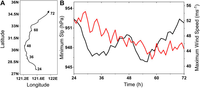
FIGURE 1. The 48-h track (A) and intensity (B) of the simulated TC in the semi-idealized experiment. The TC intensity is indicated by the minimum sea level pressure (SLP) (black, hPa) and 10-m maximum wind speed (red, ms⁻¹).

The other experiment is the prediction of Hurricane Wilma (2005) from (Chen et al., 2011). The initial and lateral boundary conditions were from then-operational GFDL model data. The details about the setup of the WRF model and the corresponding verification can be found in (Chen et al., 2011). The experiment included four interactive domains with the horizontal grid spacing of 27 km, 9 km, 3 km and 1 km, respectively, with 55 vertical levels. The output of the innermost domain at 5-min intervals is used in this study. The 72-h experiment was initialized at 0000 UTC 18 October 2005 and terminated at 0000 UTC 21 October 2005. Figure 2 shows the predicted track and intensity of Wilma after the first 18-h spin-up. The predicted storm generally takes a northwestward track. Consistent with the observation, the predicted storm experiences an initial spin-up, the rapid intensification from 18 to 36 h and the intensity change associated with the eyewall replacement during the last 36 h.

FIGURE 2

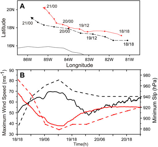
FIGURE 2. The observed (dashed) and predicted (solid) tracks (A) and intensity (B) of Hurricane Wilma (2005) during the period 1800 UTC 18 October 2005 (18 h) to 0000 UTC 21 October 2005 (72 h). The intensity is indicated by the minimum sea level pressure (SLP) (red, hPa) and 10-m maximum wind speed (black, ms⁻¹).

PVT method and TC center detection

The PV tendency in the coordinates moving with a TC is written as (Wu and Wang 2000)

$\begin{array}{c}{\left(\frac{\partial P}{\partial t}\right)}_{1m}={\left(\frac{\partial P}{\partial t}\right)}_{1f}+\overrightarrow{C}\cdot \nabla P_s,\end{array}(1)$

where subscript 1 represents the wavenumber-1 component of the PV tendency and subscripts $m$ and $f$ denote the moving and fixed reference frames relative to the TC center, respectively. $\overrightarrow{C}$ is the translation velocity of the TC, and $P_s$ is the symmetric component of PV with respect to the TC center. In (1), the Ertel PV (P) is written as

$\begin{array}{c}P=\frac{1}{\rho }\overrightarrow{\eta }\cdot \nabla {\theta }_v,\end{array}(2)$

where the absolute vorticity $\overrightarrow{\eta }=2\overrightarrow{\Omega }+\nabla \times \overrightarrow{V}$, and $\overrightarrow{\Omega }$ and $\overrightarrow{V}$ are the angular velocity of rotation of Earth and three-dimensional velocity, respectively. The total air density ($\rho$) includes the densities of dry air, water vapor, condensed water, and hydrometeors. ${\theta }_v$ is the virtual potential temperature.

In (Wu and Wang 2000), the PV tendency in the moving reference frame was neglected since it is much smaller than the one in the fixed reference frame in their study. In this study, we retain the term and calculate it with the time difference method. The PV tendency in the fixed reference frame can be calculated with the time difference or from the PV tendency equation. The gradient of the symmetric component of PV are calculated with the space difference method. The least square method is used to solve the zonal and meridional components of the translation velocity within a radius of 90 km (Wu and Wang 2000). In fact, when the calculation area covers the inner-core region, the results are insensitive to the selection of the radius since the TC translation velocity is weighed by the gradient of the symmetric component of PV.

When quantifying the contributions of individual physical processes, we use the PV tendency equation in the fixed reference as follows

$\begin{array}{c}{\left(\frac{\partial P}{\partial t}\right)}_{1f}={\wedge }_1\left(-\overrightarrow{V_h}\cdot {\mathit{\nabla }}_{h}P-w\frac{\partial P}{\partial z}+\frac{\overrightarrow{\eta }}{\rho }\cdot \mathit{\nabla }\frac{d{\theta }_v}{dt}+R\right),\end{array}(3)$

where $\overrightarrow{V_h}$ and $w$ are the horizontal and vertical components of the wind velocity. The right-hand side of (3) includes the horizontal advection (HA), vertical advection (VA), diabatic heating (DH) terms. R includes the friction term and the effects related to momentum flux. In this study, R is calculated as a residual of (3) and thus also includes the calculation error. The operator ${\wedge }_1$ is used to obtain the wavenumber one component. In addition to the PV tendency in the moving coordinates (PVTm), as indicated in (1) and (3), the TC translation velocity calculated with the PVT method can result from five physical processes: the development of the wavenumber-one component (PVTm), HA, VA, DH and R.

As indicated in (1), the symmetric and wavenumber one components with respect to the TC center are calculated in the PVT method. The accuracy of the decomposed symmetric and asymmetric components of the TC circulation depends critically on the TC center position due to strong wind speed and the associated strong radial gradient in the inner-core region (Willoughby 1992; Yang et al., 2020). Focusing on the resulting symmetric and asymmetric inner-core structures, Yang et al. (2020) evaluated four center-detecting methods that are often used in TC simulations by comparing the evolution of the small-scale track oscillation and vortex tilt. The centers detected with the four methods are the pressure centroid center (PCC), the PV centroid center (PVC), the maximum tangential wind center (MTC), and the minimum pressure variance center (MVC). They found that the maximun symmetric inner-core structures can be obtained with the MVC and MTC, while the resulting track oscillations and vortex tilt are smoother with the MVC than with the MTC. It is suggested that the MVC and MTC can be used in high-resolution simulations.

The method for detecting the MVC was described in Braun et al. (2006) and Yang et al. (2020). That is, the azimuthally-averaged variance of the pressure field in the inner core is calculated with an assumed TC center in the inner-core region until the minimum azimuthally-averaged variance is reached. The radius for calculating pressure variance is 90 km in this study. The method for detecting the MTC was described in Marks et al. (1992), Wu et al. (2006) and Reasor et al. (2013). The MTC is associated with the maximum azimuthal mean tangential wind. To reduce abrupt changes in the track oscillations, we detect the maximum azimuthal mean tangential wind in an annulus, rather than a single circle. The annulus is defined between 0.7 and 1.3 times the radius of maximum wind (RMW).

In the semi-idealized experiment, the RMW is about 30 km, and the width of the annulus is about 18 km. Figure 3 shows the comparisons of the zonal and meridional components of the translation velocity of the center at the 5-km altitude based on the data from the 9-km domain at 1-h intervals in the semi-idealized experiment. Despite the small differences, Figure 3 indicates that the TC velocity can be calculated based on both the MVC and MTC.

FIGURE 3

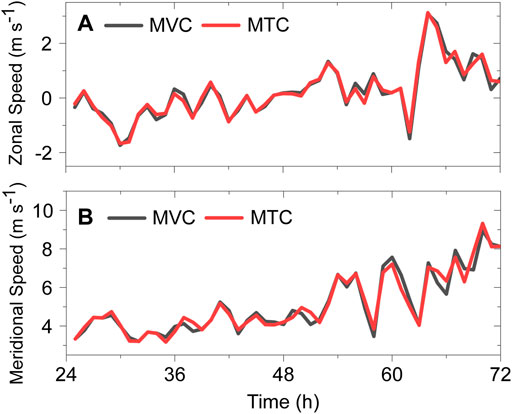
FIGURE 3. Comparisons of the zonal (A) and meridional (B) TC translation speed based on the MVC (black) and MTC (red) at the 5-km altitude. The 1-h model output in the 9-km domain is used from the semi-idealized experiment.

Failure of the PVT diagnostic method in the high-resolution simulation

We first demonstrate the failure of the PVT diagnostic method in the high-resolution simulation when the hourly model output is used. The TC translation velocity (hereafter PVT velocity) is retrieved by using the 1-h instantaneous outputs from the various model domains in the semi-idealized experiment. Note that the TC translation velocity calculated with the center position (hereafter TC velocity) at 1-h intervals are nearly identical in these domains despite the varying grid sizes (figure not shown). In this section, the MVC is used as the TC center to demonstrate that the PVT velocity can be very different when the grid sizes become smaller than 9 km.

Figure 4 shows the time series of the zonal and meridional components of the TC translation velocity retrieved with the PVT method at the 5-km altitude. The PVT tendency terms were calculated with the time difference method. As shown in Figure 4, while the PVT velocity in the 9-km domain is in good agreement with the TC velocity, the PVT method fails to retrieve the TC velocity in the 3-km, 1-km and 1/3-km domains. Moreover, as the grid size becomes finer, the PVT velocity is closer to zero.

FIGURE 4

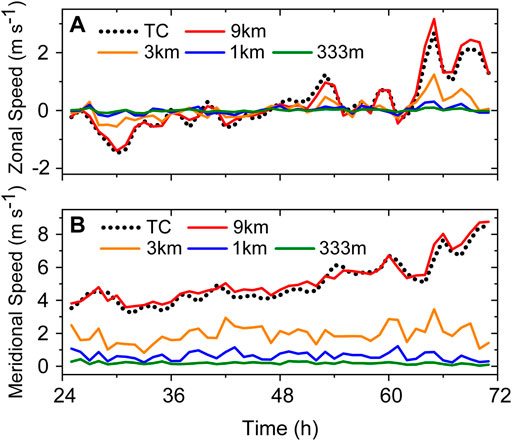
FIGURE 4. Time series of the zonal (A) and meridional (B) components of TC velocity based on the MVC (black dashed) and the PVT velocity from the 9-km domain (red), the 3-km domain (orange), the 1-km domain (blue) and the 1/3-km domain (green) at 5-km altitude in the semi-idealized experiment.

With the increase of the numerical model resolution, the simulated PV structure contains complicated small-scale structures (Ito et al., 2017; Wu et al., 2018, 2019). To understand the influence of the complicated small-scale features on the PVT method, we first conducted two experiments, in which we replaced the wave-number-one component of PVT and horizontal gradient of the symmetric PV component with those in the 1/3-km domain, respectively. By doing this we can pinpoint the influence of the complicated small-scale features. Figures 5, 6 show the comparisons of the resulting zonal and meridional components of the PVT velocity for the three selected levels, which represent the TC motion at the lower, middle and upper levels. When the wavenumber-one component of PV tendency is replaced with that in the 1/3-km domain, the TC motion can be well retrieved with the MVC and MTC. However, when the horizontal gradient of the symmetric PV component in (1) is replaced with that in the 1/3-km domain (blue), the TC motion is poorly retrieved. Both the zonal and meridional components are close to zero. It is suggested that the failure of the PVT method in the 1/3-km domain arises from the calculation of the horizontal gradient of the symmetric PV component.

FIGURE 5

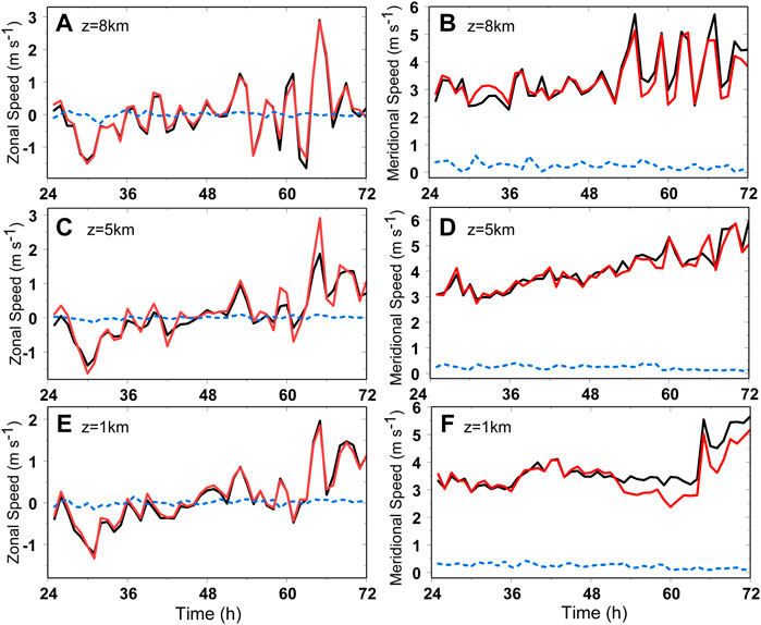
FIGURE 5. The zonal (left) and meridional (right) components of the PVT translation velocity based on the symmetric PV gradient from the 9-km domain and the wave-number-one component of PV tendency from the 1/3-km domain (red), the symmetric PV gradient from the 1/3-km domain and the wave-number-one component of PV tendency from the 9-km domain (blue), and the symmetric PV gradient from the 9-km domain and the wave-number-one component of PV tendency from the 9-km domain (black) at (A,B) 8 km, (C,D) 5 km and (E,F) 1 km in the semi-idealized experiment. The TC speed is based on the MVC.

FIGURE 6

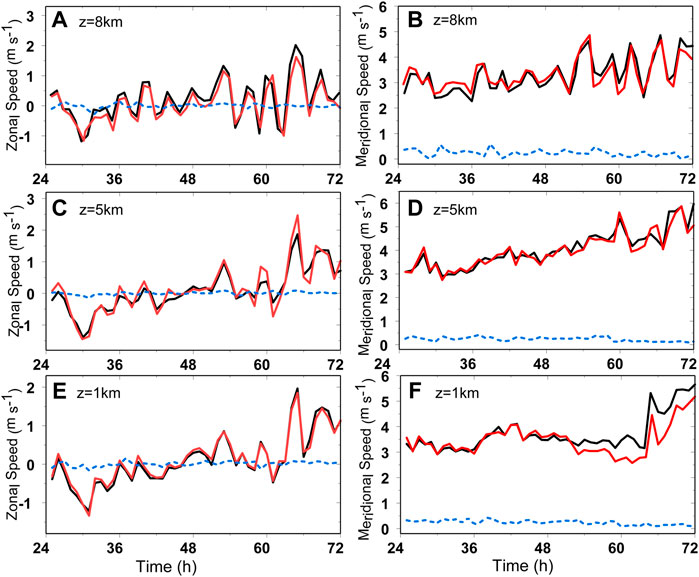
FIGURE 6. The zonal (left) and meridional (right) components of the PVT translation velocity based on the symmetric PV gradient from the 9-km domain and the wave-number-one component of PV tendency from the 1/3-km domain (red), the symmetric PV gradient from the 1/3-km domain and the wave-number-one component of PV tendency from the 9-km domain (blue), and the symmetric PV gradient from the 9-km domain and the wave-number-one component of PV tendency from the 9-km domain (black) at (A,B) 8 km, (C,D) 5 km and (E,F) 1 km in the semi-idealized experiment. The TC speed is based on the MTC.

Why cannot we use the 1-h instantaneous output to represent the horizontal gradient of PV over the 1-h period? Figure 7 shows the radius-altitude cross section of the azimuthal mean PV in the 9-km and 1/3-km domains at 48 h. In the 9-km domain, as shown in Figure 7A, the simulated TC exhibits a bowl-shaped PV anomaly within the radius of ∼30 km, extending to 12 km. The maximum of PV is more than 35 PVU (1 PVU = 10⁻⁶ kg⁻¹ K m² s⁻¹) in the eye, with large radial PV gradient in the inner side of the eyewall. The simulated PV structure agrees well with previous studies (e.g., Chen and Yau 2001; Martinez et al., 2019). As the horizontal grid spacing decreases to 1/3 km (Figure 7B), there are many small-scale features although the bowl-shaped structure can be generally identified. A significant difference is localized PV maxima in the inner side of the eyewall. Figure 8 further shows the comparison of the horizontal cross section of PV in the two domains and their difference at the 5-km altitude. Comparing with the PV in the 9-km domain (Figure 8A), there are small-scale features outside of the high-PV core (Figure 8B). The small-scale structures are clearly seen in their difference (Figure 8C). It is suggested that the presence of the small-scale features can make difference in the calculated horizontal gradient of the symmetric PV component.

FIGURE 7

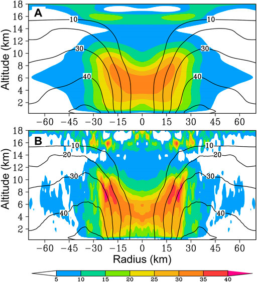
FIGURE 7. The radius-altitude cross section of the azimuthal mean PV (shaded, unit: 10^–6 m²s⁻¹ Kkg⁻¹) and the azimuthal mean wind (contour, unit: ms⁻¹) at 48 h in the semi-idealized experiment. The PV is calculated with the outputs from (A) the 9-km domain and (B) 1/3-km domain, respectively.

FIGURE 8

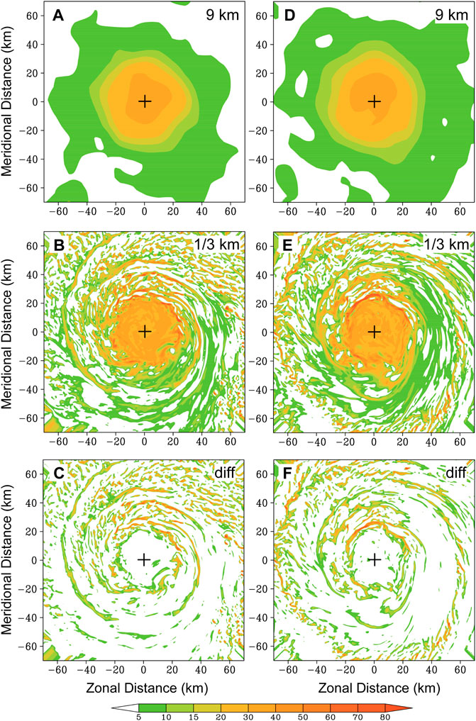
FIGURE 8. The 5-km PV (10^–6 m²s⁻¹ Kkg⁻¹) field calculated from (A,D) the 9-km domain and (B,E) the 1/3-km domain and (C,F) their difference at 48 h (left) and 57 h (right) in the semi-idealized experiment. The plus symbol denotes the position of the TC center.

Figure 9 shows the comparisons of the zonal and meridional gradients of the azimuthal mean PV calculated from the 9-km domain and the 1/3-km domain at 48 h at the altitude of 5-km in the semi-idealized experiment. Compared with the 9-km domain, the PV gradient in the 1/3-km domain exhibits complicated radial structures, which result from the azimuthal mean of the small-scale features characterized by localized high PV maxima. In other words, the symmetric PV component is distorted by the localized PV maxima when making the azimuthal average.

FIGURE 9

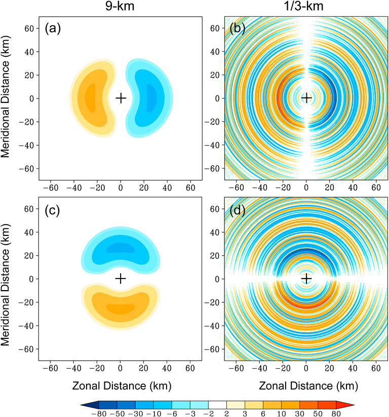
FIGURE 9. The zonal (A,B) and meridional (C,D) gradients of the azimuthal mean PV (unit: 10^–10 m²s⁻² Kkg⁻¹) calculated from the 9-km domain (left) and the 1/3-km domain (right) at 48 h at the altitude of 5-km in the semi-idealized experiment.

Improvement of the PVT method for high-resolution simulations

In the last section, we show that the presence of the small-scale PV features can distort the resulting symmetric PV component. If the simulation with the high spatial resolution can resolve the small-scale features with very high PV, the evolution of the small-scale features must be represented in the calculation of the PV tendency. On the other hand, the small-scale features must be smoothed out as the PVT method is applied to the data at longer time intervals. Thus we can have two approached to improve the PVT method for high-resolution simulations.

Increasing time intervals

Since the PV structure cannot be well resolved with the 1-h model output, we first calculated the PV tendency and TC velocities with the 2-h model output of the semi-idealized experiment at 1-min intervals. Figure 10 shows the comparison between the PVT velocity and TC velocity based on the MTC and MVC, respectively. We can see that the TC motion at 1-min intervals can be retrieved with the PVT method, the correlation coefficients of zonal and meridional velocities are 0.95 (0.80) and 0.91 (0,72) for the MTC (MVC), respectively. The fluctuations of PVT velocity with the MVC are smaller than that with the MTC. Note that the TC translation velocity from the 1-min output can also have larger errors than that from 1-h output.

FIGURE 10

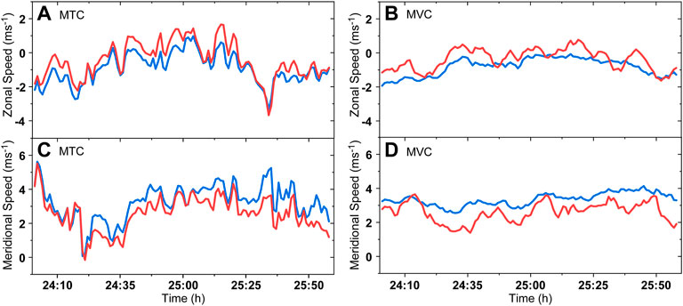
FIGURE 10. Comparisons of the zonal (A,B) and meridional (C,D) TC translation velocity derived from the TC center position (blue) and PV tendency (red) based on the MTC (A,C) and MVC (B,D) in the 1-min output and the 1/3-km domain at 5-km altitude in the semi-idealized experiment.

We also examined the retrieved PVT velocity using the prediction data of Hurricane Wilma (2005). Using the 5-min data, the TC velocity can be well retrieved with both the MTC and MVC although there are differences of the PVT velocity between the MVC and the MTC (Figure 11). For clarity, the 1-h running average is applied to the time series. Taking the MTC as an example, the zonal and meridional correlation coefficients between the TC and PVT velocities are 0.94 and 0.98, respectively. It is suggested that the TC velocity in the high-resolution simulation can be retrieved with the PVT method using the minute-interval output.

FIGURE 11

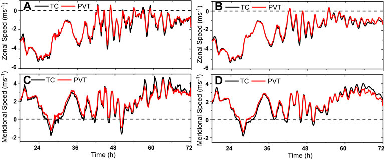
FIGURE 11. Comparisons of the zonal (A,B) and meridional (C,D) TC translation velocity derived from the TC center position (black) and PV tendency (red) based on the MTC (A,C) and MVC (B,D) of the 5-min output in the 1-km domain at 5-km altitude in the prediction of Hurricane Wilma. The 1-h running average is applied to the time series.

Reducing influence of small-scale PV features

(Zhao et al., 2019) suggested that the PVT method can be improved by smoothing the meteorological fields such as wind speed and temperature. However, the smoothing method and time were subjectively selected in (Zhao et al., 2019). In this study, a horizontal-thinning method is introduced to smooth the model output. The model output is horizontally thinned to the resolution of ∼10 km for the calculation of the PVT velocity at the interval of ∼1 h.

The thinning method can be illustrated by calculating the PVT velocity in the simulation of Hurricane Wilma. Here we use the instantaneous output in the 1-km domain at a time interval of 1 h. First, a 9-point smoothing is applied to the fields required in the PVT method, and then we have the resulting fields with the horizontal resolution of 3 km. Note that we cannot directly smooth the PV field since it is dominated by the positive PV. Second, using the smoothed fields, we repeat the first step and then we have the thinned output with the horizontal resolution of 9 km. Finally, we use the thinned, smoothed model output to calculate the PVT velocity.

Figure 12 shows the comparisons between the PVT velocity and TC velocity based on the instantaneous 1-h output in the 1-km domain. The PVT velocity is retrieved with the original output (black dashed) and thinned output (red dashed), respectively. For clarity, a 3-h running average is applied to the time series. While the PVT velocity from the original output deviates significantly from the TC velocity, the TC velocity is well retrieved from the thinned output. The correlation between the TC and PVT velocities is 0.94 and 0.95 in the zonal and meridional components, respectively. Note that we can improve the performance of the PVT method by increasing time intervals and spatially smoothing model output.

FIGURE 12

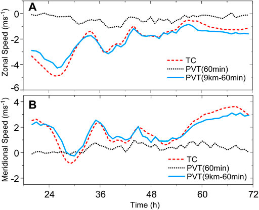
FIGURE 12. Comparisons of the zonal (A) and meridional (B) components of the TC velocity (red dashed) and the PVT velocity (blue solid) derived from the prediction of Hurricane Wilma (2005). The PVT velocity is calculated with the original 1-h output with the 1-km grid spacing (black dotted) and the corresponding thinned one (blue solid).

Diagnosing contributions of physical processes

As shown in the last section, the TC translation velocity in the high-resolution can be well retrieved by increasing the output time interval or/and thinning the model output. In this section, we show that using the PV tendency equation, we can examine the individual contributions of the five physical processes: HA, VA, DH, the development of the wavenumber-one component (PVTm), and R. Since the PVT method can retrieve the TC translation velocity with 1-km resolution predicted data of Hurricane Wilma (2005), here we use the experiment as an example to illustrate the diagnosis of the contributions from various physical processes. Figure 13 shows the contributions of the five processes to the PVT velocity at the altitudes of 1 km, 5 and 8 km at 28 h. Note that the PVT velocity at each level is the vector sum of the contributions of the five processes. Consistent with the TC velocity, the retrieved PVT velocities at the three levels are nearly the same, and direct to the southwest. The PVT velocity is dominated by the contributions of HA, VA, and DH at 5 and 8 km, while R also plays a role in the boundary layer at 1 km. Although the individual contributions vary in the vertical, the TC vortex can maintain its coherent structure in the vertical.

FIGURE 13

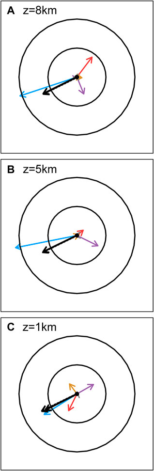
FIGURE 13. PVT velocity (black) and variations of contributions of HA (blue), VA (purple), DH (red), R (brown) and PVTm (grey) at 1 km (A), 5 km (B) and 8 km (C) at 28 h of the prediction of Hurricane Wilma. The black circles represent speeds of 3 and 6 ms⁻¹, respectively. The black dash line vector indicates the TC velocity at the same altitude.

Figure 14 further shows the time series of the contributions of the individual contributions at 5 km. Since the predicted Wilma maintains a relatively symmetric structure, the contribution of PVTm is generally small during the period, while the contribution of R increases since 60 h. As indicated in Wu and Chen (2016), the contributions of these processes are not physically independent due to the coherent structure of the TC. For example, the correlation between the contributions of VA and HA is −0.53 in the zonal component and the correlation between the contributions of VA and DH is −0.4 in the meridional component. It is suggested that the contributions of these processes to the TC motion can partially cancelled each other.

FIGURE 14

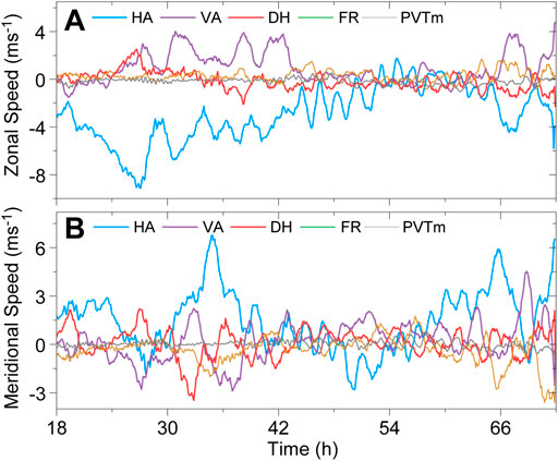
FIGURE 14. Comparisons of the zonal (A) and meridional (B) contributions of HA (blue), VA (purple), DH (red), R (brown) and PVTm (grey) terms at the 5-km altitude in the prediction of Hurricane Wilma.

Summary

As the model grid spacing decreases to ∼1 km, the PV structure of the simulated TC is an annular tower of high PV with relatively low PV in the eye and the resulting reversal of the radial PV gradient in the eyewall is subject to dynamic instability. While the PVT method has been successfully used to understand TC motion in numerical simulations with relatively coarse resolution (∼10 km), this study reevaluates the performance of the PVT diagnosis method by using the model output from two high-resolution TC simulations with grid spacing of ∼1 km.

It is indicated that the failure of the PVT method in the high-resolution simulation arises from the influence of small-scale PV features on the calculation of the horizontal gradient of the symmetric PV component. This study demonstrates that the TC translation velocity in the high-resolution can be well retrieved by increasing the output time interval and thinning the model output. As the grid spacing decreases to ∼1 km, the minute-interval model output can be used to calculate the PVT velocity. Alternatively, when the 1-h model output is available, a 9-point smoothing is successively used to thin the fields required in the PVT method, until the grid spacing of the smoothed fields is ∼10 km. The thinned model output can be used to calculate the PVT velocity.

In this study, we also demonstrate that the PV tendency can be divided into two parts: one for TC motion and the other for the development of the asymmetric structure of TCs. It is suggested that the PVT method can be useful to understand the changes of TC structure and the associated intensity.

Data availability statement

Publicly available datasets were analyzed in this study. This data can be found here: https://mygeohub.org/resources/1601.

Author contributions

LW and TX conducted analysis and writing. TX contributed to figures included in this manuscript. JY offered advices to the writing.

Acknowledgments

The detail of the predicted data of Hurricane Wilma (2005) was described in (Chen et al., 2011). The authors thank Da-Lin Zhang of University of Maryland for providing the prediction data. This study was jointly supported by the National Natural Science Foundation of China (41730961, 42192551 and 421507100531).

Conflict of interest

The reviewer YW is currently organizing a Research Topic with the author LW.

The remaining authors declare that the research was conducted in the absence of any commercial or financial relationships that could be construed as a potential conflict of interest.

Publisher’s note

All claims expressed in this article are solely those of the authors and do not necessarily represent those of their affiliated organizations, or those of the publisher, the editors and the reviewers. Any product that may be evaluated in this article, or claim that may be made by its manufacturer, is not guaranteed or endorsed by the publisher.

References

Braun, S. A., Montgomery, M. T., and Pu, Z. (2006). High resolution simulation of Hurricane Bonnie (1998). Part I: The organization of eyewall vertical motion. J. Atmos. Sci. 63, 19–42. doi:10.1175/jas3598.1

CrossRef Full Text | Google Scholar

Carr, L. E., and Elsberry, R. L. (1995). Monsoonal interactions leading to sudden tropical cyclone track changes. Mon. Weather Rev. 123, 265–290. doi:10.1175/1520-0493(1995)123<0265:miltst>2.0.co;2

CrossRef Full Text | Google Scholar

Chan, J. C. L., Ko, F. M. F., and Lei, Y. M. (2002). Relationship between potential vorticity tendency and tropical cyclone motion. J. Atmos. Sci. 59, 1317–1336. doi:10.1175/1520-0469(2002)059<1317:rbpvta>2.0.co;2

CrossRef Full Text | Google Scholar

Chen, H., Zhang, D.-L., Carton, J., and Atlas, R. (2011). On the rapid intensification of Hurricane Wilma (2005). Part I: Model prediction and structural changes. Weather Forecast. 26, 885–901. doi:10.1175/waf-d-11-00001.1

CrossRef Full Text | Google Scholar

Chen, Y., and Yau, M. K. (2001). Spiral bands in a simulated hurricane. Part I: Vortex rossby wave verification. J. Atmos. Sci. 58 (15), 2128–2145. doi:10.1175/1520-0469(2001)058<2128:sbiash>2.0.co;2

CrossRef Full Text | Google Scholar

Choi, Y., Yun, K.-S., Ha, K.-J., Kim, K.-Y., Yoon, S.-J., and Chan, J.-C.-L. (2013). Effects of asymmetric SST distribution on straight-moving typhoon ewiniar (2006) and recurving typhoon maemi (2003). Mon. Weather Rev. 141, 3950–3967. doi:10.1175/mwr-d-12-00207.1

CrossRef Full Text | Google Scholar

Duchon, C. E. (1979). Lanczos filtering in one and two dimensions. J. Appl. Meteor. 18, 1016–1022. doi:10.1175/1520-0450(1979)018<1016:lfioat>2.0.co;2

CrossRef Full Text | Google Scholar

Fovell, R. G., Corbosiero, K. L., Seifert, A., and Liou, K.-N. (2010). Impact of cloud-radiative processes on hurricane track. Geophys. Res. Lett. 37, L07808. doi:10.1029/2010GL042691

CrossRef Full Text | Google Scholar

Green, B. W., and Zhang, F. (2015). Numerical simulations of Hurricane Katrina (2005) in the turbulent gray zone. J. Adv. Model. Earth Syst. 7, 142. doi:10.1175/JAS-D-14-0244.1

CrossRef Full Text | Google Scholar

Hong, S.–Y., Lim, J., and Kim, J-H. (2006). The WRF single–moment 6–class microphysics scheme (WSM6). J. Korean Meteor. Soc. 42, 129.

Google Scholar

Hsu, L.-H., Kuo, H.-C., and Fovell, R. G. (2013). On the geographic asymmetry of typhoon translation speed across the mountainous island of taiwan. J. Atmos. Sci. 70, 1006–1022. doi:10.1175/jas-d-12-0173.1

CrossRef Full Text | Google Scholar

Ito, J., Oizumi, T., and Niino, H. (2017). Near-surface coherent structures explored by large eddy simulation of entire tropical cyclones. Sci. Rep. 7, 3798. doi:10.1038/s41598-017-03848-w

PubMed Abstract | CrossRef Full Text | Google Scholar

Kain, J. S., and Fritch, J. M. (1993). Convective parameterization for mesoscale models: The kain–fritch scheme. The representation of cumulus convection in numerical models. Meteorol. Monogr. 46, 165–170. doi:10.1007/978-1-935704-13-3_16

CrossRef Full Text | Google Scholar

Lander, M. A. (1994). Description of a monsoon gyre and its effects on the tropical cyclones in the Western North Pacific during August 1991. Wea. Forecast. 9, 640–654. doi:10.1175/1520-0434(1994)009<0640:doamga>2.0.co;2

CrossRef Full Text | Google Scholar

Liang, J., and Wu, L. (2015). Sudden track changes of tropical cyclones in monsoon gyres: Full-physics, idealized numerical experiments. J. Atmos. Sci. 72, 1307–1322. doi:10.1175/jas-d-13-0393.1

CrossRef Full Text | Google Scholar

Marks, F. D., Houze, R. A., and Gamache, J. F. (1992). Dual-aircraft investigation of the inner core of Hurricane Norbert. Part I: Kinematic structure. J. Atmos. Sci. 49, 919–942. doi:10.1175/1520-0469(1992)049<0919:daioti>2.0.co;2

CrossRef Full Text | Google Scholar

Martinez, J., Bell, M. M., Rogers, R. F., and Doyle, J. D. (2019). Axisymmetric potential vorticity evolution of hurricane patricia (2015). J. Atmos. Sci. 76 (7), 2043–2063. doi:10.1175/jas-d-18-0373.1

CrossRef Full Text | Google Scholar

Menelaou, K., Yau, M. K., and Lai, T.-K. (2018). A possible three-dimensional mechanism for oscillating wobbles in tropical cyclone–like vortices with concentric eyewalls. J. Atmos. Sci. 75 (7), 2157–2174. doi:10.1175/jas-d-18-0005.1

CrossRef Full Text | Google Scholar

Mirocha, J. D., Lundquist, J. K., and Kosović, B. (2010). Implementation of a nonlinear subfilter turbulence stress model for large-eddy simulation in the advanced research WRF model. Mon. Weather Rev. 138, 4212–4228. doi:10.1175/2010mwr3286.1

CrossRef Full Text | Google Scholar

Möller, J. D., and Smith, R. K. (1994). The development of potential vorticity in a hurricane-like vortex. Q. J. R. Meteorol. Soc. 120, 1255–1265. doi:10.1002/qj.49712051907

CrossRef Full Text | Google Scholar

Montgomery, M. T., and Shapiro, L. J. (1995). Generalized charney–stern and fjortoft theorems for rapidly rotating vortices. J. Atmos. Sci. 52 (10), 1829–1833. doi:10.1175/1520-0469(1995)052<1829:gcaftf>2.0.co;2

CrossRef Full Text | Google Scholar

Noh, Y., Cheon, W. G., Hong, S.-Y., and Raasch, S. (2003). Improvement of the K-profile model for the planetary boundary layer based on large-eddy simulation data. Bound. Layer. Meteorol. 107, 401–427. doi:10.1023/a:1022146015946

CrossRef Full Text | Google Scholar

Reasor, P. D., Rogers, R., and Lorsolo, S. (2013). Environmental flow impacts on tropical cyclone structure diagnosed from airborne Doppler radar composites. Mon. Weather Rev. 141, 2949–2969. doi:10.1175/mwr-d-12-00334.1

CrossRef Full Text | Google Scholar

Rotunno, R., Chen, Y., Wang, W., Davis, C., Dudhia, J., and Holland, G. J. (2009). Large-Eddy simulation of an idealized tropical cyclone. Bull. Am. Meteorol. Soc. 90, 1783–1788. doi:10.1175/2009bams2884.1

CrossRef Full Text | Google Scholar

Schubert, W. H., Montgomery, M. T., Taft, R. K., Guinn, T. A., Fulton, S. R., Kossin, J. P., et al. (1999). Polygonal eyewalls, asymmetric eye contraction, and potential vorticity mixing in hurricanes. J. Atmos. Sci. 56, 1197–1223. doi:10.1175/1520-0469(1999)056<1197:peaeca>2.0.co;2

CrossRef Full Text | Google Scholar

Wang, C.-C., Chen, Y.-H., Kuo, H.-C., and Huang, S.-Y. (2013). Sensitivity of typhoon track to asymmetric latent heating/rainfall induced by taiwan topography: A numerical study of typhoon fanapi(2010). J. Geophys. Res. Atmos. 118, 3292–3308. doi:10.1002/jgrd.50351

CrossRef Full Text | Google Scholar

Willoughby, H. E. (1992). Linear motion of a shallow-water barotropic vortex as an initial-value problem. J. Atmos. Sci. 49, 2015–2031. doi:10.1175/1520-0469(1988)045<1906:LMOASW>2.0.CO;2

CrossRef Full Text | Google Scholar

Wong, M. L. M., and Chan, J. C. L. (2006). Tropical cyclone motion in response to land surface friction. J. Atmos. Sci. 63, 1324–1337. doi:10.1175/jas3683.1

CrossRef Full Text | Google Scholar

Wu, L., Braun, S. A., Halverson, J., and Heymsfield, G. (2006). A numerical study of Hurricane Erin (2001). Part I: Model verification and storm evolution. J. Atmos. Sci. 63, 65–86. doi:10.1175/jas3597.1

CrossRef Full Text | Google Scholar

Wu, L., and Chen, X. (2016). Revisiting the steering principal of tropical cyclone motion in a numerical experiment. Atmos. Chem. Phys. 16, 14925–14936. doi:10.5194/acp-16-14925-2016

CrossRef Full Text | Google Scholar

Wu, L., Liu, Q., and Li, Y. (2018). Prevalence of tornado-scale vortices in the tropical cyclone eyewall. Proc. Natl. Acad. Sci. U. S. A. 115, 8307–8310. doi:10.1073/pnas.1807217115

PubMed Abstract | CrossRef Full Text | Google Scholar

Wu, L., Liu, Q., and Li, Y. (2019). Tornado-scale vortices in the tropical cyclone boundary layer: Numerical simulation with the WRF–LES framework. Atmos. Chem. Phys. 19, 2477–2487. doi:10.5194/acp-19-2477-2019

CrossRef Full Text | Google Scholar

Wu, L., and Wang, B. (2000). A potential vorticity tendency diagnostic approach for tropical cyclone motion. Mon. Wea. Rev. 128, 1899–1911. doi:10.1175/1520-0493(2000)128<1899:apvtda>2.0.co;2

CrossRef Full Text | Google Scholar

Wu, L., and Wang, B. (2001b). Effects of convective heating on movement and vertical coupling of tropical cyclones: A numerical study. J. Atmos. Sci. 58, 3639–3649. doi:10.1175/1520-0469(2001)058<3639:eochom>2.0.co;2

CrossRef Full Text | Google Scholar

Wu, L., and Wang, B. (2001a). Movement and vertical coupling of adiabatic baroclinic tropical cyclones. J. Atmos. Sci. 58, 1801–1814. doi:10.1175/1520-0469(2001)058<1801:mavcoa>2.0.co;2

CrossRef Full Text | Google Scholar

Wu, L., Zong, H., and Liang, J. (2013). Observational analysis of tropical cyclone formation associated with monsoon gyres. J. Atmos. Sci. 70, 1023–1034. doi:10.1175/jas-d-12-0117.1

CrossRef Full Text | Google Scholar

Yang, H., Wu, L., and Xie, T. (2020). Comparisons of four methods for tropical cyclone center detection in a high-resolution simulation. J. Meteorological Soc. Jpn. 98, 379–393. doi:10.2151/jmsj.2020-020

CrossRef Full Text | Google Scholar

Yu, H., Huang, W., Duan, Y. H., Chan, J. C. L., Chen, P. Y., and Yu, R. L. (2007). A simulation study on pre-landfall erratic track of typhoon Haitang (2005). Meteorol. Atmos. Phys. 97, 189–206. doi:10.1007/s00703-006-0252-1

CrossRef Full Text | Google Scholar

Zhao, J., Xie, T., Yang, H., Wu, L., and Liu, Q. (2019). Application of PVT method for diagnosing typhoon motion with high-resolution data. Acta Meteorol. Sin. 77, 1062. doi:10.11676/qxxb2019.065

CrossRef Full Text | Google Scholar

Zhu, P., Menelaou, K., and Zhu, Z. (2013). Impact of subgrid-scale vertical turbulent mixing on eyewall asymmetric structures and mesovortices of hurricanes: Impact of SGS vertical turbulent mixing on eyewall asymmetries. Q. J. R. Meteorol. Soc. 140, 416–438. doi:10.1002/qj.2147

CrossRef Full Text | Google Scholar

Zhu, P. (2008). Simulation and parameterization of the turbulent transport in the hurricane boundary layer by large eddies. J. Geophys. Res. 113, D17104. doi:10.1029/2007jd009643

CrossRef Full Text | Google Scholar