Analysis of storm surge events along the Norwegian coast

1 Introduction

Because of the potential for flooding of highly urbanized coastal areas with both dense, expensive infrastructure and high population density, storm-surges (StSs) are considered an economic and safety hazard (Munich RE, 2019). This risk is projected to increase dramatically due to future sea-level rise and socio-economic developments (Hallegatte et al., 2013). For necessary climate adaptation planning by decision makers, an in-depth knowledge of the mechanisms steering the heights of StSs is thus relevant. This study assesses the interplay between astronomical tides (ATs) and StSs based on local sea level (SL) measurements from tide gauges (TGs) along the Norwegian coastline, together with storm track data over the North Atlantic region.

Typically, extreme water levels are estimated in terms of return levels. Return levels are the water levels that will be exceeded with a specific very low probability in a given year, approximately corresponding the occurrence of the event once in a set number of years. 100 years return event, for instance, would be a water level occurring in a single year with the probability corresponding to it occurring once in 100 years. These are calculated with different methods applying extreme value statistics (Haigh et al., 2010). So-called direct methods use extreme value analysis of SL observations of between a few decades to 100 years length in order to calculate the return levels (e.g., Simpson et al., 2017). In Norway, a slightly unusual direct method, the average conditional exceedance rate (ACER) statistical method (Næss and Gaidai, 2009) is found to be the most suitable for estimating extreme sea level return periods (Haug, 2012; Skjong et al., 2013). The method has also been successfully adopted for calculating sea level allowances together with projections of future sea level rise (Simpson et al., 2015; 2017).

The problem with direct approaches is that the interaction between ATs and StSs is not considered in the calculation of the return levels. In the comparatively short measurement records extreme SL measurements could be biased by the fact that StSs may have occurred during comparatively low ATs, while combinations of high ATs and StSs are possible over longer time spans. The so-called indirect methods are specifically designed to mitigate this shortcoming by using separate statistics for ATs and StSs and considering the overlap of both phenomena. It is thus argued that shorter SL records can be used for a more precise estimation of return values since all so far occurred StS heights are considered and ATs can be predicted through harmonic functions (Haigh et al., 2010). In Norway, as in many countries around the world, return levels based on direct measurements are the basis of the national building standards, regulating at what height infrastructure can be built.

Recent studies using TG observations have focused on the relevance of the so-called “near misses” (Dangendorf et al., 2016; Haigh et al., 2016). These are situations where an extreme StS coincides with an AT that is below the highest astronomical tide, i.e. the elevation of the highest predicted astronomical tide expected to occur at a specific tide station based on any combination of astronomical conditions. While the occurrence of a moderate AT in combination with an extreme StS can lead to record-breaking sea levels, the co-occurrence with the highest astronomical tide could have made the flooding far more devastating. This can also lead to a significant shift in the expected return levels, highlighting the instability of SL extreme value statistics (Dangendorf et al., 2016). Moreover, dynamical modeling based studies also showed (potential) effects of various constellations of storms and tidal phases on historical (Horsburgh et al., 2021) and on future water level extreme events (Grabemann I., et al., 2020). In this work, with a special focus on the Norwegian coastline, we address the question of whether or not there is a need to assess the components that give rise to extreme sea level events independently? We also address the question of how storm tracks and the passage of storms shape the observed extreme sea level events?

Because of their limitations, statistical techniques can be conveniently complemented by deterministic approaches. Deterministic approaches are designed to identify the drivers of extreme sea-level events in coastal areas (Ganske et al., 2018), and they are useful from a coastal adaptation perspective because they quantify the impact of possible, though highly unlikely, extreme sea-level events in coastal areas (Ganske et al., 2018; Wei et al., 2019; Horsburgh et al., 2021). A notable example is presented in Horsburgh et al., (2021). They showed that variations in the intensity and position of storm Xavier, which hit northern Europe in December 2013, could have led the sea level to exceed the observed values by up to 1.5 m at some locations.

In this paper, we adopt a deterministic approach by focusing on the overlap between ATs and StSs for the generation of SL extremes. In addition, we attempt to understand the relevance of single storms on the extremes caused. Our findings suggest that the two-parameter system treated with the indirect measurements may still underestimate the maximum possible combination of ATs and StSs. The StS itself is dependent both on the location and the strength of the passing storm systems. Thus, it may be useful to treat the two-parameter system of ATs and StSs rather as a three-parameter system of ATs, storm location, and strength.

The manuscript is structured as follows: Section 2 describes the data and methods, while the results are presented in Section 3. Section 4 presents the discussion and conclusions, setting the results into the perspective of the existing literature.

2 Data and methods

2.1 Tide gauge measurements

For the analysis of the SL height along the Norwegian coast we used data from 21 of the 23 permanent Norwegian TGs operated by the Norwegian Mapping Authority (http://api.sehavniva.no/tideapi_no.html). We use the entire available record for each of the TGs with a 10 min measurement interval (Figure 1). This dataset contains observed SLs and the predicted ATs. Two permanent TGs are not included in this study: Oslo (too short high-frequency data record) and Mausund (large gap in the record). For each TG we detrended the SL and AT by removing the respective linear trend of the entire record length. The maximum difference between the original and the processed SL was small (6.2 cm at Narvik and below 4.3 cm elsewhere). The maximum difference for AT was less than 1 cm at any station. In Norway the mean SL rise has so far been much smaller than for other countries, largely due to the glacial isostatic adjustment after the melting of the Fennoscandinavian ice sheet. For some of the stations the mean SL trend is negative, while the maximum was around 1 mm/yr for the 1960–2010 period (Richter et al., 2012). We detrended AT (no mean trend since calculated from harmonic analysis) in order to make it fully comparable to the SL. The AT could be in a different phase at the beginning and end of the datasets, creating a small apparent trend in both datasets.

FIGURE 1

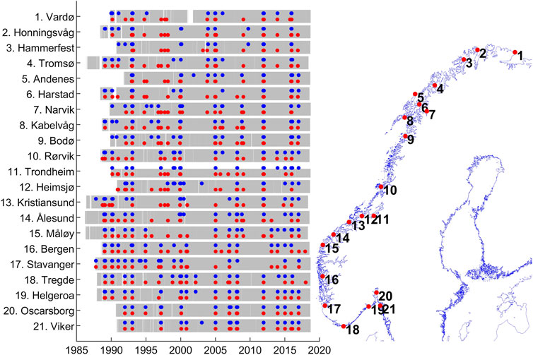
FIGURE 1. Overview over the 21 permanent tide gauges. Left: Data availability for each TG in grey. Cases of extreme sea level and extreme skew surge are marked with red and blue dots, respectively. Right: Location of the TGs along the Norwegian coastline (from EEA, 2018).

2.2 Skew surges

Apart from land motion, the observed SL consists of three contributions: mean sea-level, astronomical tide, and weather effects (e.g. Haigh et al., 2016). To quantify the weather effect on the SL we use the frequently applied concept of skew surges (SkS) (e.g. de Vries et al., 1995). The SkS is the difference between the maximum observed SL and the maximum predicted AT during each tidal cycle irrespective of their temporal offset. The concept of SkS is commonly preferred over that of non-tidal residual, which is the difference between the observed SL and the predicted AT each instant in time, because it helps better assess the impact of storms in coastal areas. Coastal dwellers are indeed concerned by the residual relative to the maximum in sea level that would be experienced in the absence of a meteorological forcing (e.g., Horsburgh et al., 2010; Pugh and Woodworth, 2014) a high non-tidal residual would have a little flooding effect if the corresponding observed SL exceeded the maximum high tide by only a few centimeters.

The mean SL is influenced by two factors, the mean SL over a longer averaging period, e.g. monthly means, and of a possible long-term trend (see Section 2.1). For simplicity we will not discuss separately the longer-term trend, as it can have multiple causes, such as long-term ocean variability or changes in the inflow into ocean basins from large-scale weather modes (e.g., Richter et al., 2009, 2012). These possible contributions are thus part of the diagnosed SkS heights.

In our analysis of the TG data we reduced the 10 min datasets to full tidal cycles (approximately 12 h). We used the full 10-min dataset for the identification of the SkS values. For this we first identified the AT cycles searching for all n AT maxima at points in time {T₁, … , T_n} for each dataset. To be identified as a maximum a peak’s prominence must be at least 5 cm. We calculated the SkSs for each tidal cycle defined as lasting from time (T _k-1+T_k)/2 until (T_k+1+T_k)/2, with k∈{2, … , n-1}. Tidal cycles are therefore not defined as equally spaced 12 hourly time intervals but as the time intervals between tidal minima. The remaining analysis is done on this dataset with reduced frequency. Each time step is now defined at the maximum of the respective tidal cycle. For the identification of extreme cases of SLs and SkSs we used a 99.9th percentile threshold, high enough to give a manageable number of cases. Finally, we applied a criterion that any two distinct extremes must be separated by at least four tidal cycles (≈48 h).

2.3 Storm tracks

For the analysis of the effect of cyclones on the SL, we used the storm track dataset described in Chen et al., (2016) for the period between 1979 and 2013. This dataset is based on the relative vorticity at 850 hPa in the ERA-Interim reanalysis (Dee et al., 2011). A storm track here refers to the path of a single storm described by the location of the storm center points and its intensity described by the 850 hPa relative vorticity at the storm’s center point with a 6 hourly temporal resolution using the TRACK algorithm developed by Hodges (1999). To be more comparable to the higher temporal resolution TG dataset, we increased the temporal resolution of the identified storm tracks to 1.5 h using linear interpolation of the 6-h latitude-longitude positions. This was necessary since the storm center points should be related to specific SL extremes in the approximately 12 hourly dataset (reduced from 10 min data as described in Section 2.2 above). The storm centers and SL extremes would have been mismatched if the storm track dataset were used in its original 6 hourly format.

3 Results

3.1 Interplay between the different components creating high sea levels and skew surges

We would like to better understand the relative contribution of SkS and AT to the generation of SL extremes along the Norwegian coast. Figure 1 marks the cases exceeding the 99.9th percentile of the SLs and SkSs. A clustering appears to exist for some cases affecting the entire Norwegian coast with both extremes in SL and SkS. However, closer inspection revealed that these were often cases that occurred within a few weeks of each other and not at the same time. Only the case during January 1993 affected the entire Norwegian coast with extreme SL. Only the TGs south of Heimsjø were affected by an extreme SkS simultaneously, and no single case exists where all TGs were affected by extreme SkSs simultaneously. Investigating the January 1993 case revealed, at the Bergen TG for example, that the AT exceeded the 97.0 percentile of all AT maxima and reached 87.6% of the highest astronomical tide, while the SkS exceeded the 99.9 percentile but only reached 68.9% of the highest observed SkS. In short, a rare and high AT coincided with a very rare but only moderately high SkS at the Bergen TG. Further north the storm’s relative influence weakened compared to other StSs at the respective TGs. One possible explanation of this is the propagation of the storm along the entire Norwegian coast, causing extreme SLs together with the very high AT. Other cases only affected parts of the TG network, suggesting that the storms’ influences in those cases were more confined to only parts of the Norwegian coast.

Different combinations of AT and SkSs are assessed in more detail in Figure 2. In this figure, we have isolated the 99.9th percentile of SL events (left column for each TG, black), and the 99.9th percentile of extreme SkS events (right column for each TG, red). Each event is shown with its SL (black), AT (blue), and SkS (red), thus any single SL event is shown with AT and SkS which sum up to produce that SL. Along the coast the extreme SLs follow high ATs. One exception is in the area near the amphidromic point in Southern Norway (Gjevik, 2009; Simpson et al., 2015), where there are hardly any tides, as seen in the last five stations on the right side of Figure 2. Northward from Stavanger, ATs and extreme SLs generally increase, with a slight reversal between Narvik and Harstad (across the Lofoten islands) only to increase again further northward. A division into approximately the same regions is also seen for SkSs, which are strong in the southeast, increasing in the west (after a slight decrease), and rather similar levels among the stations north of Narvik and the Lofoten archipelago. The distinct change in the tidal regime across the Lofoten islands is caused by the local bathymetry and described in more detail in Moe et al., [ 2002].

FIGURE 2

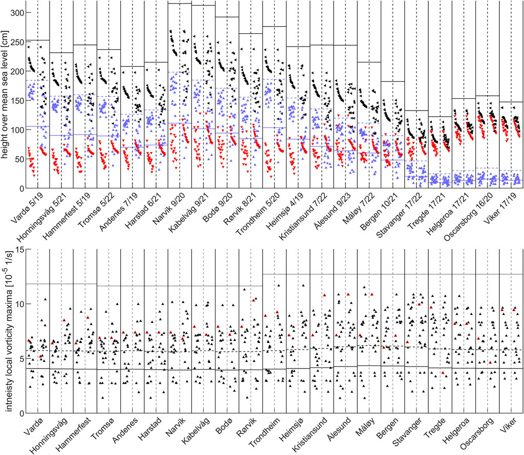
FIGURE 2. Upper panel: Observed SL maxima (black), SkS maxima (red) and AT maxima (blue) during each tidal cycle. Left and right columns for each TG show the 99.9th percentile of the SL maxima and SkSs, respectively. Numbers after the station names state the number of cases, where the 99.9th percentile is exceeded for both SkSs and the observed SL during a period ± 48 h from each other/the total number of cases, where the 99.9th percentile is exceeded for SkSs only. Blue lines mark the mean (solid) and maximum observed (dashed) AT for each TG. Black lines mark the maximum combination of AT and SkS irrespective of temporal overlap. Lower panel: Storm intensities of the nearest center point for the same cases as above. The cases with the highest observed SL (left column) and SkS (right column) are marked in red. The black lines mark the mean (solid), mean + 1 standard deviation (dashed), and maximum (dotted) storm track intensity within 500 km from each TG.

For all TGs with maximum ATs as high as or higher than the maximum SkSs, less than half of the extreme SkSs coincide with extreme SLs, indicating that most of the extreme SL came from the AT. ATs and SkSs only overlapped in magnitude consistently for the stations in Southern Norway (c.f. Kristiansund to Bergen). As an example, the maximum AT Narvik is the highest of all TGs and so is the maximum observed sea level. During cases with extreme SL, the AT reached a maximum of 175 cm (highest blue point, left column). The maximum AT in the entire dataset reached 180 cm (where the highest astronomical tide is 180 cm). Simultaneously, the maximum SkS was 122 cm (highest red point, right column) but the highest SkS during any of the cases of extreme SL was 111 cm (highest red point, left column), which is more than 10 cm lower than the highest SkS. In fact, the case with the highest SkS had a maximum AT of only 81 cm, leading the SL to be only 203 cm or 64 cm lower than the highest SL. This illustrates the situation that is found at most of the stations, that the cases with the highest SkSs typically coincided with moderately high ATs, while the cases with the highest SLs only coincided with moderately high SkSs. The numbers after the TG names in Figure 2 reinforce this conclusion by showing how many of the cases of extreme SL occurred with extreme SkSs. For example, at the first station at Vardø, 19 cases were identified as having SL at the 99.9th percentile, but only 5 of these events had SkSs which were also at the 99.9th percentile, meaning 14 extreme SL cases occurred without an extreme in SkS.

Often, this mismatch between AT and SkS is considered expected due to the inverse relationship between the water depth and the SkS height for shallow shelves. However, under these assumptions a consistent time-lag should exist between the maxima of AT and SL, and along the Norwegian coast, no such time-lag exists (see Supplementary Material). It is therefore plausible for any AT to occur with any SkS, as was shown by Williams et al., (2016) for the UK coast, thus opening the possibility for far more extreme SL events to occur given the right combination of AT and SkS.

Assuming the highest observed SkS at Narvik would have coincided with the highest astronomical tide, this would have led to a sea level of 320 cm or 53 cm higher than the maximum observed SL (Figure 2, black solid line). A similar picture is visible for most TGs with the highest astronomical tide as high as or higher than the maximum observed SkSs. Thus, the solid black lines for each TG in Figure 2 indicate the SL that would have been reached if the highest SkS had occurred with the highest astronomical tide, and their height above the highest black mark for each TG indicates how much more the extreme SL could have been if the two had co-occurred. This is based purely on the observations of the past 30–35 years. Exceptions are Andenes, Harstad, Tromsø and Vardø, where the maximum SL nearly reached the maximum possible combination of ATs and SkSs. A different picture is also visible for the stations in Southern Norway, e.g., Stavanger onwards. Here AT is very low and thus, the combination with the highest SkSs and the highest astronomical tides is not far above the maximum observed SL.

So far, we only treated the maximum possible SL as a system with two factors, AT and SkS. However, the SkS itself is influenced by numerous effects, primarily the effect of storm systems near the TG. Storms exert a direct effect on the sea level through both the inverse barometric effect and the wind forcing, and upon meeting the coastline as a barrier for the water they form storm surges. Other factors that we neglect in this work include for example waves from storm systems far away from TGs (e.g. Benoit Cushman-Roisin & Beckers, 2011; Dangendorf et al., 2016). Based on the inverse barometric effect, a storm’s impact on the SkSs can be described by the strength of a storm system and the location of the storm itself. The lower panel of Figure 2 shows the strength of the storms that were closest to each TG during extreme SLs or SkSs. Intensity does not seem to vary much along the coastline, but there is a clear difference north and south of Trondheim/Rørvik with slightly higher maxima occurring near the TGs in the southern half of the Norwegian coast. Extreme (exceeding the 99.9th percentile) SLs or SkSs rarely coincided with the maximum nearby observed storm intensity and in many cases even coincided with storms of below average intensity. Even the single cases with the highest SL or SkS did not coincide with particularly high storm intensities.

Again, using Narvik as an example, the storm with the highest intensity near to Narvik in the entire dataset had an intensity that is around 42% stronger than the nearest storm during the case with the highest SkS. While the effect of the storm intensity on SkS may not be linear, it is safe to say that a such strong increase in intensity may lead to a stronger SkS assuming all other factors (e.g., location) unchanged.

3.2 Storm track locations

Figure 3 shows the storm tracks during extreme SkSs. From this, TGs may be separated into two categories, all TGs north of and including Trondheim and those south of and including Heimsjø. The storm tracks temporally coinciding with extreme SkSs at the northern Norwegian TGs mostly pass northeastward through the North Atlantic Ocean at some distance along the Norwegian coast. Eventually they ‘glance’ the coast, impacting the respective TGs before the storms pass on into the Barents Sea. The storm tracks coinciding with extreme SkSs at the southern Norwegian TGs more often cross Norway at the latitude of the respective TGs. One exception to this is the northernmost TG, at Vardø. Storms connected to extreme SkSs there must intersect Norway since Vardø is sheltered from the North Atlantic and thus the typical storm tracks by Northern Norway.

FIGURE 3

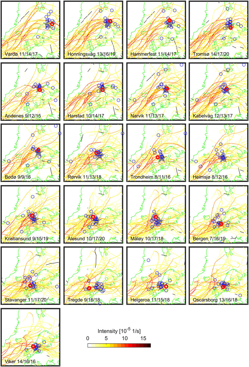
FIGURE 3. Storm tracks for the 99.9th percentile SkS for each TG. Blue rings mark the nearest storm center point at the time of each SkS maximum (occurred ± 6 h of the maximum AT). Red rings mark the center points for the highest SkSs in the dataset. Storm track colors indicate their intensity. The location of TGs is marked with a grey star. The numbers next to the station name give the number of SkSs with storm center points closer than 500 km/1,000 km/all cases.

For most TGs, the nearest storm track centers temporally coinciding with extreme SkSs are less than 500–1,000 km away from each TG. The centers for the northern TGs are either located to the north or west of the stations in accordance with a storm traveling along the Norwegian coastline, meaning these storms are mostly glancing the coast at the respective stations. For the southern Norwegian TGs, the center points are often distributed around the stations or directly atop of them. Most of the storm tracks show weak to moderate intensities, consistent with the analysis of the intensity of the center points closest to the observed extreme SkSs in Figure 2.

The center point positions during the highest SkSs for each TG are marked with red circles in Figure 3. They are mostly located close to the TGs, suggesting that both the barometric effect and the wind forcing played a role for the height of the related StSs. For Heimsjø no storm track could be found, since the highest SkS occurred later than the extent of the storm track record. For Narvik the closest center point during the highest SkS was located over Svalbard. This storm likely did not directly trigger an extreme SL at Narvik due to the large distance of its center from the TG. We do not know why this SkS reached such a high level. Possibly a cyclone or a polar low could have been missed by the TRACK algorithm or SkS could have been caused purely by other phenomena.

4 Discussion and conclusion

The proposed independence of StSs from ATs motivating our study is in agreement with the study by Williams et al., (2016). They propose such independence for most of the TGs along the U.K. coast. This would enable a simple convolution of the return frequencies for extreme StSs and extreme ATs for assessment of the return frequencies for plausible extreme SL events outside of the SL statistics observed. Furthermore, the TGs at Andenes, Harstad, Tromsø and Vardø confirm this hypothesis, since very high ATs coincided with very high StSs.

As an example of what this implies, at the Bergen TG the same distribution of SkS events but a re-sampling of the single incidences leads to a maximum possible SL extreme of 182 cm (Figure 2, horizontal solid black line in Bergen column). Such a SL exceeds the currently highest observed SL in Bergen that occurred on 27 February 1990 by 32 cm. Furthermore, under the RCP8.5 scenario future mean SL rise around Bergen is projected to be 53 cm by 2,100 (Norwegian Mapping and Cadastre Authority, 2019; Simpson et al., 2015), on top of which our possible maximum SL extreme event would reach 235 cm, which is 15 cm above the Norwegian national building code standard for critical infrastructure of 220 cm (National Office of Building Technology and Administration, 2019). It should be restated that the possible extreme event of 182 cm would only be produced by the coincidence of the highest astronomical tide and the largest SkS seen in the last 35 years. Such an event may be rarer than the 1000 year return frequency that the national building code level for Bergen is defined at. The probabilities of such an event occurring could be assessed for Bergen and for each tide gauge in Norway individually using joint probabilities, though this is not covered here and will be the focus of future work.

Similar approaches for the definition of extreme floods due to coinciding high ATs and SkSs have been adapted to the U.K. (Haigh et al., 2010; Tawn, 1992), and referred to as indirect methods for the inference of return values. An important part of the correct statistical treatment is a reduction of the likelihood of the highest possible overlaps due to mismatches in the occurrences of extreme ATs (mostly around the solstice points) and extreme SkSs (mostly in winter). Without performing a thorough examination of the return periods for Norway by different methods (which is beyond the scope of this paper), we can instead highlight specific situations during the 30 year database that would have exceeded the 1000 year return level for Bergen. This return level was calculated using direct extreme value statistics to be 148 cm (Simpson et al., 2015). The highest ever observed SL in Bergen was 150 cm on 27 February 1990. The SkS and AT the time of this event were 77.0 cm and 73.0 cm, respectively. During the last 30 year record this AT was exceeded 154, 111, and 66 times during December, January and February or on average around 5, 4, and 2 times per month during the last 30 year record, and the SkS level was exceeded once during each December, January and February. This suggests that an overlap of ATs and SkSs exceeding the current estimate of the 1000 year return level for Bergen is very possible and that we already here can identify so-called “near misses” (Dangendorf et al., 2016; Haigh et al., 2016).

Such near misses are of course much more likely considering the rather short datasets available for the analysis of extreme sea level events. Due to the desire to use high frequency - high quality automated measurements for this work, the length of the available dataset is severely limited. Simultaneously, the datasets on which the Norwegian building code is based are not much longer. The return levels for the Norwegian TGs in Simpson et al., (2015) were calculated from record lengths typically less than 79 years and maximum 100 years, equal or less than 10% of the target 1000-year return period. A repetition of the analysis presented in this publication with datasets spanning up to 100 years would be desirable, if suitable data were available. A longer dataset would allow the conclusions on the coincidence between ATs and SkSs to be tested since it should show a wider variety of possible combinations Ats and SkSs. However, the possibility for such super-flooding may be better assessed using paleo reconstructions which have far longer records. Some historic records might exist of extreme events for the last several hundred years, for example from the Hanseatic activity in Bergen. Possible weaknesses in the return-level calculations based on an only 100 years-long data series was highlighted during a StS event on 11 February 2020, where the maximum SL of 149 cm was reached in Bergen. The 1000 years return level has thus been exceeded twice in 30 years. Even though much of this increase in occurrences can be attributed to long term SL rise, it does suggest that indirect methods may be more desirable.

There is a need to mention the large spatial variability of possible exceedances of return levels and national building code thresholds. The strongest recorded SkS for Oscarsborg nearby Oslo (123 cm, record length of 29 years) together with the projected mean SL rise in the RCP8.5 scenario (28 cm) and highest AT in the record (28 cm) would be 186 cm, 47 cm below the national building code threshold of 233 cm relative to the mean sea level from 1996 to 2014. The national building code threshold would not be exceeded, even using the 95% confidence interval for the mean sea level rise of 61 cm. The relevance of the coincidence between AT and SkS is strongly reduced since the Oslo area shows one of the strongest isostatic adjustments and the AT amplitude is low due to its proximity to the amphidromic point.

It is clear that future studies are needed to uncover what independence between AT and SkS means for extreme SL events along the Norwegian coastline. The role of storms and their paths and strength is also important to discuss. There appears to be a separation of storm tracks, as seen by two typical main paths of single storms relative to the Norwegian coastline, affecting extreme SkSs at stations north of Trondheim and south of Heimsjø. This can be linked to the analysis of Chafik et al., (2017) despite a focus on different time scales. They found monthly mean extreme SL (detrended, seasonalized and the inverse barometric effect removed) in Bergen to coincide with a mean sea level pressure pattern with a maximum over central Germany and a minimum southwest of Iceland. For SL extremes in Tromsø the maximum was located over Denmark and the minimum over Southeast Greenland. This resulted in monthly mean winds crossing Norway over Bergen or propagating further along the Norwegian coast, similar to the storm tracks in our analysis. The observed ‘glancing’ of the Norwegian coast at the location of the TGs is therefore a result of the shape of the Norwegian coastline with a meridional orientation in Southern Norway and a more zonal orientation in Northern Norway. A northward or southward shift in the pressure pattern causes the isolines either to follow the Norwegian coast or cross it, respectively. Chafik et al., (2017) attributed the extreme monthly mean SLs in Bergen to a positive North Atlantic Oscillation (NAO) modulated by a positive East Atlantic Pattern and neutral Scandinavian Pattern. The extreme monthly mean SLs at Tromsø they attributed also to a positive NAO, modulated by a light positive East Atlantic Pattern and a negative Scandinavian Pattern. The positive NAO is consistent with the typical mean storm track location over Norway, compared to the more southern mean storm tracks for a negative NAO phase (Bader et al., 2011; Trigo, 2006).

In order to better understand extreme sea-level events in a region with such a complex geometry such as the Norwegian coast, it is important to make the connection between SL events and the specific properties of extratropical cyclones rather than connecting them with storm tracks or large scale pressure patterns. We know from the literature that storm intensity, location, size, and speed of propagation can greatly affect the risk and impact of flooding in coastal areas (e.g., Jelenianski, 1972; Azam et al., 2004; Benavente et al., 2006; Haigh et al., 2016; Wei et al., 2019). However, to the authors’ knowledge, the combination of different storms’ properties along the coast of Norway has not been addressed by the literature. For example, the intensity of storms is associated with the strength of wind stress over the ocean and could be related to anomalously high sea-level events. However, the intensities of storms have to be considered in relationship with their paths. The path followed by a storm affects the wind pattern in coastal areas and, therefore, can determine whether water piles up or not along certain portions of the coast (Andrée et al., 2022). A future study could follow Dangendorf et al. (2016) and propose an analysis of storm surges that takes into consideration ATs, storms’ location, and the storms’ strengths. Or, it could exploit other deterministic approaches, such as those in Ganske et al. (2018) and Horsburgh et al. (2021), for example, using a high-resolution numerical model to reproduce the impact of a storm from the past, and understand how it changes as some of the cyclone’s characteristics are modified.

Data availability statement

Publicly available datasets were analyzed in this study. This data can be found here: Coastline dataset from the European Environment Agency (©EEA). Tide gauge data and predicted tides are provided by the Norwegian Mapping Authority licensed under Creative Commons Attribution 4.0 international (CC BY 4.0). The tide gauge data can be accessed from the Norwegian Mapping Authority's website using their API at https://www.kartverket.no/en/api-and-data/tidal-and-water-level-data.

Author contributions

Scientific concept, analysis, and writing by TW Scientific concept and writing by SO Data and scientific discussions by LC and JN Scientific discussions with FM.

Funding

This research has been supported by the Utdannings- og forskningsdepartementet (Basic funding to Bjerknes Centre for Climate Research) through the Climate Hazards and Extremes (CHEX) strategic project of the Bjerknes Centre for Climate Research.

Acknowledgments

The authors thank the European Environment Agency for the coastline dataset (©EEA). Tide gauge data and predicted tides are provided by the Norwegian Mapping Authority licensed under Creative Commons Attribution 4.0 international (CC BY 4.0).

Conflict of interest

The authors declare that the research was conducted in the absence of any commercial or financial relationships that could be construed as a potential conflict of interest.

Publisher’s note

All claims expressed in this article are solely those of the authors and do not necessarily represent those of their affiliated organizations, or those of the publisher, the editors and the reviewers. Any product that may be evaluated in this article, or claim that may be made by its manufacturer, is not guaranteed or endorsed by the publisher.

Supplementary material

The Supplementary Material for this article can be found online at: https://www.frontiersin.org/articles/10.3389/feart.2023.1037826/full#supplementary-material

References

Andrée, E., Drews, M., Su, J., Larsen, M. A. D., Drønen, N., and Madsen, K. S. (2022). Simulating wind-driven extreme sea levels: Sensitivity to wind speed and direction. Weather Clim. Extrem. 36, 100422. doi:10.1016/j.wace.2022.100422

CrossRef Full Text | Google Scholar

Azam, M.H., Samad, M.A., and Mahboob-Ul-Kabir, (2004). Effect of cyclone track and landfall angle on the magnitude of storm surges along the coast of Bangladesh in the northern Bay of Bengal. Coastal engineering journal 46 (03), pp.269–290. doi:10.1016/j.atmosres.2011.04.007

CrossRef Full Text | Google Scholar

Bader, J., Mesquita, M. D. S., Hodges, K. I., Keenlyside, N., Østerhus, S., and Miles, M. (2011). A review on northern hemisphere sea-ice, storminess and the North atlantic oscillation: Observations and projected changes. Atmos. Res. 101 (4), 809–834. doi:10.1016/j.atmosres.2011.04.007

CrossRef Full Text | Google Scholar

Chafik, L., Nilsen, J., and Dangendorf, S. (2017). Impact of North Atlantic teleconnection patterns on northern European sea level. J. Mar. Sci. Eng. 5 (3), 43. doi:10.3390/jmse5030043

CrossRef Full Text | Google Scholar

Chen, L., Fettweis, X., Knudsen, M., and Johannessen, O. M. (2016). Impact of cyclonic and anticyclonic activity on Greenland ice sheet surface mass balance variation during 1980. Int. J. Climatol. 36, 3423–3433. doi:10.1002/joc.45652013December 2015

CrossRef Full Text | Google Scholar

Cushman-Roisin, Benoit, and Beckers, J.-M. (2011). Introduction to geophysical fluid dynamics, physical and numerical aspects. 2nd ed. Cambridge, MA, USA: Academic Press. https://www.elsevier.com/books/introduction-to-geophysical-fluid-dynamics/cushman-roisin/978-0-12-088759-0.Retrieved from

Google Scholar

Dangendorf, S., Arns, A., Pinto, J. G., Ludwig, P., and Jensen, J. (2016). The exceptional influence of storm ‘Xaver’ on design water levels in the German Bight. Environ. Res. Lett. 11 (5), 054001. doi:10.1088/1748-9326/11/5/054001

CrossRef Full Text | Google Scholar

de Vries, H., Breton, M., de Mulder, T., Krestenitis, Y., Ozer, J., and Proctor, R., (1995). A comparison of 2D storm surge models applied to three shallow European seas. Environ. Softw. 10 (1), 23–42. doi:10.1016/0266-9838(95)00003-4

CrossRef Full Text | Google Scholar

Dee, D. P., Uppala, S. M., Simmons, a. J., Berrisford, P., Poli, P., and Kobayashi, S., (2011). The ERA-interim reanalysis: Configuration and performance of the data assimilation system. Q. J. R. Meteorological Soc. 137 (656), 553–597. doi:10.1002/qj.828

CrossRef Full Text | Google Scholar

Eea, (2018). EEA coastline for analysis. Retrieved from https://www.eea.europa.eu/data-and-maps/data/eea-coastline-for-analysis-2#tab-metadata July 4, 2019).

Google Scholar

Ganske, A., Fery, N., Gaslikova, L., Grabemann, I., Weisse, R., and Tinz, B. (2018). Identification of extreme storm surges with high-impact potential along the German North Sea coastline. Ocean. Dyn. 68, 1371–1382. doi:10.1007/s10236-018-1190-4

CrossRef Full Text | Google Scholar

Gjevik, B. (2009). Flo og fjære - langs kysten av Norge og Svalbard. Oslo: Farleia Forlag.

Google Scholar

Grabemann, I., L, Gaslikova, T, Brodhagen, and E, Rudolph (2020). Extreme storm tides in the German Bight (North Sea) and their potential for amplification. Natural Hazards and Earth System Sciences, 20(7), 1985–2000. doi:10.3390/jmse5030043

CrossRef Full Text | Google Scholar

Haigh, I. D., Nicholls, R., and Wells, N. (2010). A comparison of the main methods for estimating probabilities of extreme still water levels. Coast. Eng. 57 (9), 838–849. doi:10.1016/j.coastaleng.2010.04.002

CrossRef Full Text | Google Scholar

Haigh, I. D., Wadey, M. P., Wahl, T., Ozsoy, O., Nicholls, R. J., and Brown, J. M., (2016). Spatial and temporal analysis of extreme sea level and storm surge events around the coastline of the UK. Sci. Data 3 (1), 160107. doi:10.1038/sdata.2016.107

PubMed Abstract | CrossRef Full Text | Google Scholar

Hallegatte, S., Green, C., Nicholls, R. J., and Corfee-Morlot, J. (2013). Future flood losses in major coastal cities. Nat. Clim. Change 3 (9), 802–806. doi:10.1038/nclimate1979

CrossRef Full Text | Google Scholar

Haug, E. (2012). “Extreme value analysis of sea level observations,”. Technical Report DAF 12-1 (Stavanger, Norway: Norwegian Mapping Authority, Hydrographic Service), 180.January

Google Scholar

Hodges, K. I. (1999). Adaptive constraints for feature tracking. Mon. Weather Rev. 127 (6), 1362–1373. doi:10.1175/1520-0493(1999)127<1362:ACFFT>2.0.CO;2

CrossRef Full Text | Google Scholar

Horsburgh, K., Haigh, I. D., Williams, J., De Dominicis, M., Wolf, J., and Inayatillah, A., (2021). “Grey swan” storm surges pose a greater coastal flood hazard than climate change. Ocean. Dyn. 71 (6), 715–730. doi:10.1007/s10236-021-01453-0

CrossRef Full Text | Google Scholar

Horsburgh, K., T, Ball, B, Donovan, and G, Westbrook, (2010). Coastal flooding, MCCIP Annual Report Card 2010-11. Lowestoft, Marine Climate Change Impacts Partnership. (MCCIP Summary Report 2010).

Google Scholar

Jelesnianski, C.P. (1972). SPLASH I: Landfall Storms. NOAA Technical Memorandum NWS-TDL 46. Silver Spring, Maryland, NWS Systems Development Office.

Google Scholar

J, Benavente, L, Del Río, FJ, Gracia, and JA, Martínez-del-Pozo (2006). Coastal flooding hazard related to storms and coastal evolution in Valdelagrana spit (Cadiz Bay Natural Park, SW Spain), Continental Shelf Research. Coastal engineering journal 26 (09), pp.1061–1076. doi:10.1016/j.csr.2005.12.015

CrossRef Full Text | Google Scholar

Moe, H., Ommundsen, A., and Gjevik, B. (2002). A high resolution tidal model for the area around the Lofoten Islands, northern Norway. Cont. Shelf Res. 22, 485–504. doi:10.1016/s0278-4343(01)00078-4

CrossRef Full Text | Google Scholar

Munich, R. E. (2019). Storm surges. Retrievedfrom https://www.munichre.com/touch/naturalhazards/en/naturalhazards/hydrological-hazards/flood/storm-surges/index.html August 28, 2019).

Google Scholar

Næss, A., and Gaidai, O. (2009). Estimation of extreme values from sampled time series. Struct. Saf. 31, 325–334. doi:10.1016/j.strusafe.2008.06.021

CrossRef Full Text | Google Scholar

National Office of Building Technology and Administration, (2019). Byggteknisk forskrift (TEK17). Retrievedfrom https://dibk.no/byggereglene/byggteknisk-forskrift-tek17/7/7-2/July 10, 2019).

Google Scholar

Norwegian Mapping and Cadastre Authority, (2019). Se havnivå. Retrievedfrom https://www.kartverket.no/en/sehavniva/Lokasjonsside/?cityid=9000002&city=Bergen#tab2 July 10, 2019).

Google Scholar

Pugh, D., and Woodworth, P. (2014). sea-level science. Sea-level science - understanding tides, surges, tsunamis and mean seasea-level changes. Cambridge, MA, USA: Cambridge University Press. doi:10.1017/CBO9781139235778

CrossRef Full Text | Google Scholar

Richter, K., Furevik, T., and Orvik, K. A. (2009). Effect of wintertime low-pressure systems on the Atlantic inflow to the Nordic seas. J. Geophys. Res. 114 (C9), C09006. doi:10.1029/2009JC005392

CrossRef Full Text | Google Scholar

Richter, K., Nilsen, J. E. Ø., and Drange, H. (2012). Contributions to sea level variability along the Norwegian coast for 1960-2010. J. Geophys. Res. Oceans 117 (C5). doi:10.1029/2011JC007826

CrossRef Full Text | Google Scholar

Simpson, M. J. R., Nilsen, J. E. Ø., Ravndal, O. R., Breili, K., Sande, H., and Kierulf, H. P., (2015). sea level change for Norway - past and present observations and projections to 2100. Retrieved from https://www.miljodirektoratet.no/globalassets/publikasjoner/M405/M405.pdf.

Google Scholar

Simpson, M. J. R., Ravndal, O., Sande, H., Nilsen, J., Kierulf, H., and Vestøl, O., (2017). Projected 21st century sea-level changes, observed sea level extremes, and sea level allowances for Norway. J. Mar. Sci. Eng. 5 (3), 36. doi:10.3390/jmse5030036

CrossRef Full Text | Google Scholar

Skjong, M., Næss, A., and Næss, O. E. B. (2013). Statistics of extreme sea levels for locations along the Norwegian coast. J. Coast. Res. 29, 1029–1048. doi:10.2112/jcoastres-d-12-00208.1

CrossRef Full Text | Google Scholar

Tawn, J. (1992). Estimating probabilities of extreme sea-levels. J. R. Stat. Soc. Ser. C Appl. Statistics) 41 (1), 77–93. doi:10.2307/2347619

CrossRef Full Text | Google Scholar

Trigo, I. F. (2006). Climatology and interannual variability of storm-tracks in the euro-atlantic sector: A comparison between ERA-40 and NCEP/NCAR reanalyses. Clim. Dyn. 26 (2–3), 127–143. doi:10.1007/s00382-005-0065-9

CrossRef Full Text | Google Scholar

Wei, X., Brown, J. M., Williams, J., Thorne, P. D., Williams, M. E., and Amoudry, L. O. (2019). Impact of storm propagation speed on coastal flood hazard induced by offshore storms in the North Sea. Ocean. Model. 14, 101472. doi:10.1016/j.ocemod.2019.101472

CrossRef Full Text | Google Scholar

Williams, J., Horsburgh, K. J., Williams, J. A., and Proctor, R. N. F. (2016). Tide and skew surge independence: New insights for flood risk. Geophys. Res. Lett. 43 (12), 6410–6417. doi:10.1002/2016GL069522

CrossRef Full Text | Google Scholar