Evolution of total column ozone prior to the era of ozone depletion

1 Introduction

The Earth’s ozone layer has undergone large changes in the past 60 years (WMO, 2018). A period of rapid ozone decline due to chlorofluorocarbons (CFCs), culminating in the 1990s (Solomon, 1999), gave way to a period of stabilisation and, recently, signs of a slow recovery in certain regions of the stratosphere (e.g., Solomon et al., 2016; Steinbrecht et al., 2018; SPARC/IO3C/GAW, 2019; Weber et al., 2022). However, there are still unresolved questions regarding trends in the lower stratosphere (e.g., Ball et al., 2020; Orbe et al., 2020; Dietmüller et al., 2021; Bognar et al., 2022) that may relate to both chemical and dynamical causes. These questions also prompt a look back in order to study trends from earlier periods.

However, while changes in total column ozone that occurred in the last 50 years or so have been well studied, the evolution of stratospheric ozone prior to the era of ozone depletion has rarely been assessed. Egorova et al. (2020) recently analyzed changes in the 1910–1940 period using a model. A recent analysis of CMIP6 model simulations indicated a strong positive trend of total column ozone in the pre-CFC era, specifically in the latitude band 30–60°N (Keeble et al., 2021; Zeng et al., 2022), but weaker in other latitude bands. This raises the question whether a strong trend is also found in the historical observations, most of which are from the latitude band 30–60°N. Here, I address this question using historical observations and a data assimilation approach.

Regular total column ozone measurements began in 1924, when Dobson started the observations in Oxford, which he continued for more than half a century, albeit with gaps (Dobson and Harrison, 1926). There are only few long, homogenized series, namely, Arosa (Staehelin et al., 1998), Oxford (Brönnimann, 2022), and Tromsø (Hansen and Svenøe, 2005). Many total column ozone series began in 1957 in the context of the International Geophysical Year (IGY), which, however, cover only little of the pre-CFC era. A large number of per-IGY ozone series was compiled by Brönnimann et al. (2003), but many of them are relatively short fragments. Further sources of information are long series of spectral transmission in the visible wavelength range performed by the Smithsonian Institution in their solar observations program, from which ozone can be calculated using the Chappuis band (Angione and Roosen, 1983). However, these observations carry a large level of uncertainty.

Trends in the pre-CFC era have not been addressed systematically in these records. Brönnimann (2022); analyzing Oxford and Arosa, found an increase of ca. 2 DU over the 1926–1970 period. A positive trend in total column ozone until the late 1960s was already discussed by contemporary scientists (Komhyr et al., 1971). Shindell and Faluvegi (2002) found a trend of −7.2 ± 2.3 DU during 1957–1975; the latter part of the period is, however, already affected by ozone depletion. Trend analyses are further complicated by the fact that instruments and procedures changed at the start of the IGY and that, at urban locations, interference with SO₂ or effects of aerosols might affect the long-term stability of the total column ozone series (De Muer and De Backer, 1992). Here, I revisit all available early observations and complement them with some newly digitized series in order to characterize the evolution of stratospheric ozone in the 1924–1963 period. This 40-year period should be long enough to capture trends. It ends before ozone depletion is expected to have a strong contribution and before the eruption of Mt. Agung. Furthermore, I use all series in a data assimilation approach to reconstruct zonal mean total column ozone back to 1924. Notably, all available data sources have considerable uncertainties. Some even come with a note that they should not be used for trend analysis. However, by compiling as many series as possible and combining them with model simulations, thereby accounting for errors and possible inhomogeneities as far as possible and characterizing the different contributions to uncertainty, a more robust assessment is possible.

The article is organized as follows: Section 2 introduces the observational datasets used; first, the station data (some of which are newly digitized, and some are compiled from previous digitization efforts) and then the satellite data. The data assimilation approach and its evaluation are then introduced, and the analyses of all data products are outlined. Section 3 shows the results of the assimilation procedure and that of the analysis of the data products. In Section 4, the consistency of the results is assessed, given the large uncertainties in the data, and the results are compared with those found for CMIP6 models. Conclusions are drawn in Section 5.

2 Data and methods

2.1 Historical station column ozone data

The paper starts from an earlier compilation I used to produce an assimilated, two-dimensional (latitude-height) ozone dataset back to 1924 (Brönnimann et al., 2013, termed HISTOZ, hereafter). The compilation comprises long series from Arosa, Oxford, and Tromsø , as well as shorter, pre-IGY series (Brönnimann et al., 2003) and series available from the World Ozone and Ultraviolet radiation Data Centre (WOUDC). I re-assessed the homogenized series, as is further described in Section 2.5. This collection was complemented by recently digitized segments from Oxford (13 further monthly means, Brönnimann 2022), Wellington, NZ (86 months), and Downham Market (11 months, Bröninmann and Nichol, 2020). Here, I also considered data from the Smithsonian Institution from Montezuma (Angione and Roosen, 1983), although these are clearly of lower quality.

Based on scanned historical data sheets from Environment Canada, I was able to further extend some of the series. This concerns series from Reykjavik (extended by 2 months; note that also the remainder of the series was not in HISTOZ), Edmonton (14 months), and Aspendale (24 months). Furthermore, I replaced the Halley Bay series from WOUDC (as used in HISTOZ) with the series from the British Antarctic Survey (BAS), which reaches a year further back. I also added the series from Faraday from the BAS record. Furthermore, I corrected an error in the Delhi data, which had an incorrect conversion of the scale.

In order to calculate a monthly mean, it required 10 days with measurements, as in HISTOZ. This accounts for the fact that total column ozone could not be measured under all weather conditions but retains sufficient information for a monthly mean (Brönnimann, 2022). In particular, for the series from the Smithsonian Institution, with often only weekly measurements, this led to a considerable reduction of data points. For further processing, some of the non-homogenized series were segmented. This was performed to avoid artificial trends due to inhomogeneities (segments are treated independently) and is one way of accounting for the large uncertainties in the records. Segments were defined when instrument types changed or at instances of long gaps (see Supplementary Table S1). Segments or series shorter than 8 months were ignored.

A map of all stations is shown in Figure 1; the temporal coverage is shown in Figure 2. Station names, coordinates, the number of values, assigned errors, and segmentation are shown in Supplementary Table S1. The new compilation has more data than HISTOZ. Although the difference may not seem large, coverage is now considerably better in the Southern Hemisphere.

FIGURE 1

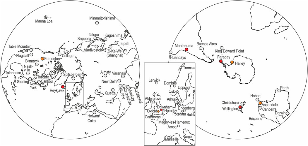
FIGURE 1. Map of series (grey: used in HISTOZ, red: new series, and orange: supplemented series).

FIGURE 2

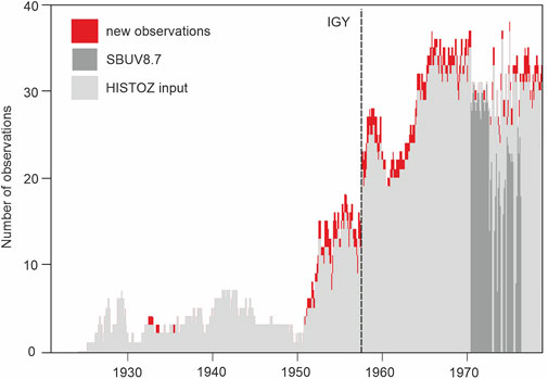
FIGURE 2. Number of historical monthly means assimilated from 1924 to 1978.

2.2 Satellite column ozone data

Although the focus of this paper is on the 1924–1963 period, I produced an assimilated dataset until 1978, which can be merged with existing data, and until 1999 for evaluation. Hence, the paper also describes the data used after 1963. In addition to the station data from WOUDC, as described in HISTOZ, I used SBUV V8.7 zonal mean total column ozone from Nimbus 4 (Ziemke et al., 2021; HISTOZ used V8). Finally, I supplemented station series that do not have data after 1978 with total column ozone data from the NIWA dataset (Bodeker et al., 2021; HISTOZ used TOMS V8).

2.3 Data assimilation

The observed segmented total column ozone data were assimilated into an ensemble of historical chemistry climate model simulations to produce a zonal mean total column ozone dataset. It is to be noted that for consistency with HISTOZ, I also produced a 2D (latitude-height) dataset of an ozone number density, which is, however, not the focus here and only shown in one plot. The collection of the new datasets is termed HISTOZ2.

The assimilation procedure followed that of HISTOZ (Brönnimann et al., 2013). I used the same set of nine all-forcing simulation of the 20th century (Fischer et al., 2008) performed with the SOCOLv2 model (Schraner et al., 2008). These simulations prescribed sea-surface temperatures, as well as all external forcings. Notably, the quasi-biennial oscillation (QBO) was nudged (Brönnimann et al., 2007). The simulations may appear rather old; however, the simulations are well-validated, and they were already used in HISTOZ. To the best of my knowledge, there are no newer sets of simulations with prescribed sea-surface temperature covering the entire 20th century. It is later shown that the agreement with the NIWA dataset is very good.

The assimilation was performed with an offline ensemble Kalman filter approach, which is briefly explained in the following. Historical total column ozone observations y were assimilated into a set of simulations x_b, yielding the assimilated dataset x_a. The ensemble mean was updated first and then anomalies from the mean.

$\overline{{\mathbf{x}}_{\mathbf{a}}}=\overline{{\mathbf{x}}_{\mathbf{b}}}+\mathbf{K}\left(\overline{\mathbf{y}}-\mathbf{H}\overline{{\mathbf{x}}_{\mathbf{b}}}\right),(1)$

${\mathbf{x}}_{\mathbf{a}}^{\prime }={\mathbf{x}}_{\mathbf{b}}^{\prime }+\stackrel{\sim }{\mathbf{K}}\left({\mathbf{y}}^{\prime }-\mathbf{H}{\mathbf{x}}_{\mathbf{b}}^{\prime }\right)=\left(\mathbf{I}-\stackrel{\sim }{\mathbf{K}}\mathbf{H}\right){\mathbf{x}}_{\mathbf{b}}^{\prime },\mathrm{w}\mathrm{i}\mathrm{t}\mathrm{h}:{\mathbf{y}}^{\prime }=0.(2)$

H is the Jacobian matrix of the linear observation operator that extracts total column ozone from the model state vector. The Kalman gain matrices K for the ensemble mean and $\stackrel{\sim }{\mathbf{K}}$ for the anomalies from the mean are defined as

$\mathbf{K}={\mathbf{P}}^{\mathbf{b}}{\mathbf{H}}^{\mathbf{T}}{\left(\mathbf{H}{\mathbf{P}}^{\mathbf{b}}{\mathbf{H}}^{\mathbf{T}}+\mathbf{R}\right)}^{-1},(3)$

$\stackrel{\sim }{\mathbf{K}}={\mathbf{P}}^{\mathbf{b}}{\mathbf{H}}^{\mathbf{T}}{\left[{\left(\sqrt{\mathbf{H}{\mathbf{P}}^{\mathbf{b}}{\mathbf{H}}^{\mathbf{T}}+\mathbf{R}}\right)}^{-1}\right]}^{\mathbf{T}}\times {\left(\sqrt{\mathbf{H}{\mathbf{P}}^{\mathbf{b}}{\mathbf{H}}^{\mathbf{T}}+\mathbf{R}}+\sqrt{\mathbf{R}}\right)}^{-1},(4)$

where P^b and R are the background error and observation error covariance matrices, respectively.

The state vector x_b was the zonal mean total column ozone (or 2D ozone number density) from the model simulations. As in HISTOZ, the vector comprised 6 months, and therefore, an ozone observation in 1 month can affect the neighboring months. The 6-month seasons (Nov–Apr and May–Oct) were defined so as to capture the active phases of the northern and southern Brewer–Dobson circulations, respectively.

A few aspects of the procedure were improved as compared to HISTOZ. Rather than calculating the covariance matrix for time t only from the nine members available at time t, I also calculated a covariance matrix from all members in all years in the 1924–1973 period, the covariance matrix P^b is then composed of the average of the two covariance matrices. This approach has proven to be beneficial in other off-line data assimilation projects (Valler et al., 2022).

In the standard version of the assimilation, termed TOZ, the background state vector x_b, for a given time t, was taken from the nine ensemble members at time t. I termed this background TOZ_b. As a further change to HISTOZ, I produced an additional dataset TOZ_c, which started from an alternative x_b consisting, for every time step, of all the members of all the years (1924–1973). As in the standard approach, each member is updated. This means that TOZ_c has a time independent prior and does not see the specific forcings of a specific year. Therefore, its time evolution is independent of TOZ_b (see schematic representation, Supplementary Figure S2). In the limiting case of no observations, TOZ would be identical to TOZ_b (the pure model simulations), while TOZ_c would be time invariant. Its time evolution is thus solely determined by observations.

Since the state vector x_b has zonally averaged quantities, while most of the observations (except SBUV from Nimbus 4) are point observations, the station data needed to be adjusted to the zonal mean, as described in HISTOZ. This was based on the deviation of local 200 hPa geopotential height from its zonal mean. As a change to HISTOZ, I used 20CRv2 (Slivinski et al., 2019) rather than a reconstruction. All observation segments were then debiased according to the overlap with TOZ_b. This can be seen as an alternative to homogenization to avoid the effect on inhomogeneities on trends.

I used the same observation errors as in HISTOZ. The new series were assigned errors of 8 DU (as for most other stations) except Reykjavik [16 DU, due to the lower quality assessed in Brönnimann et al. (2003)] and the Smithsonian measurements at Montezuma (24 DU, very low quality).

To summarize, the generated products were the prior TOZ_b, which are the pure model simulations (nine members), the full assimilation TOZ (nine members), the assimilation with a time-independent (climatological) prior TOZ_c (9 members x 50 years = 450 members in total, only ensemble mean is published), and a 2D version of the ozone number density for the full assimilation (nine members). Also, I generated a version of TOZ that was debiased relative to the NIWA dataset based on the 1978–1999 period such that it can be used as its backward extension (see Table 1).

TABLE 1

TABLE 1. Products generated and used in this paper. Obs. = observations; n = number of members.

2.4 Evaluation

Evaluation of the assimilated dataset was performed against the NIWA dataset using the mean-squared error skill score (MSESS, termed RE in HISTOZ). For this, reconstruction was continued for the period 1979–1999. This evaluation was performed, on one hand, for the post-1979 observation dataset and, on the other hand, for a subset of stations mimicking the dataset in 1942 (seven stations, all in the Northern Hemisphere).

The MSESS compares the error of reconstruction with that of a no-knowledge prediction x₀. Often, x₀ is taken to be climatology. I used the climatology of TOZ_b in the evaluation period 1924–1963 as x₀. This comparison is suitable for both TOZ and TOZ_c. However, for TOZ, it is also interesting to use an alternative x₀, such as TOZ_b (the pure model simulations). Then, the MSESS measures how much the assimilation of the observations improves over the pure model.

2.5 Analysis

In the first visualization step, each ozone series was analyzed individually. Only series with a minimum of 60 datapoints were considered the data were deseasonalized within the 1924–1963 period by fitting the first harmonic of the annual cycle. Anomalies were then filtered with a 28-month moving average, designed to minimize the effect of the QBO. Series were plotted of at least 14 of the 28 months are available. I also calculated linear least-squares trends on all deseasonalized series within the 1924–1963 period.

The data from the Smithsonian Institution were analyzed similarly. For this, deseasonalization was performed on the level of daily values (hence, I used the first two harmonics); the 28-month filter was then calculated if at least 30 daily values were available. The Montezuma series showed step jumps. As a consequence, two periods (1923–1925 and 1942–1947) were removed. Again, it should be noted that the uncertainty in the Smithsonian data is very large.

The zonal mean column ozone values from the assimilation datasets were then processed in the same way but deseasonalized based on the true mean annual cycle as sufficient data were available. Finally, the NIWA dataset was also processed and analyzed in the same way. As a reference period, I used the entire length of the dataset, i.e., 1979–2016.

The assimilated zonal mean annual mean column ozone datasets were analyzed statistically. Trends were calculated for each latitude band. Then, a linear regression approach, largely following Brönnimann (2022), was used to account for the effects of atmospheric circulation and solar UV. The following predictors were used: zonal mean 200 hPa geopotential height (Slivinski et al., 2019), the QBO at 50 hPa (Brönnimann et al., 2007) from May to October, solar UV radiation (Lean, 2018), a measure of the strength of the polar vortex at 200 hPa in December to April defined as the difference between geopotential height at 75–90°N and 45–55°N (taken from Brönnimann, 2022), and a June-to-February average of the El Niño index NINO4. The latter was taken from NOAA/PSD, which is the average of the sea surface temperature in the region [5° N–5° S 160° E−150° W] from HadISST1. This analysis was conducted for all products (TOZ, TOZ_b, and TOZ_c) and for all ensemble members, as well as the ensemble mean. Then, the trend of the residuals was analyzed.

A very similar regression model (but using local rather than zonal mean 200 hPa height as a proxy for local tropopause heights and using the additional variable equivalent stratospheric chlorine and methane; see Brönnimann (2022) for a full description of the model) was applied to the long, homogenized series of Arosa, Oxford, and Tromsø. I then analyzed and filtered the residual with a 10-year moving average as a visual check for inhomogeneities (Supplementary Figure S1). The series show no obvious signs of inhomogeneities, but there are large interannual and multiannual variations.

3 Results

A plot of the smoothed observations (Figure 3B) shows no visual evidence for strong trends. However, there is considerable interannual-to-multiannual variability. Specifically, I find a strong spike in the early 1940s that was described previously and was related to a strengthened Brewer–Dobson circulation induced by an El Niño event (Brönnimann et al., 2004). In fact, plotting the NINO4 index (Figure 3A) indicates that spikes in 1952 and 1958 coincided or followed El Niño events. The Smithsonian series from Table Mountain follows the same pattern, while that from Montezuma seems to behave in an opposite way (Figure 3C). This is expected since Montezuma is in the tropics, and hence, changes in the strength of the Brewer–Dobson circulation would have the opposite effect (note, again, the large uncertainty in this series).

FIGURE 3

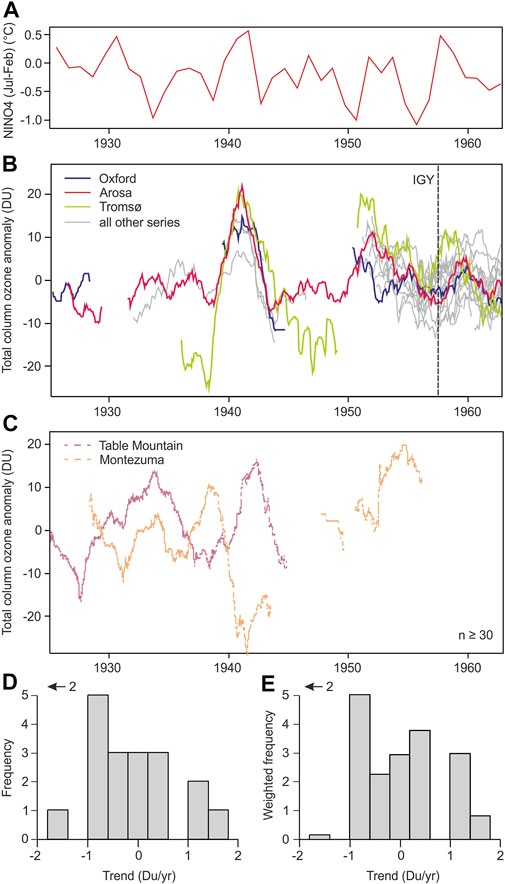
FIGURE 3. (A) Time series of NINO4; (B, C) total column ozone anomalies (calculated per segment), filtered with a 28-month moving average (B: Dobson data and (C) Smithsonian data); (D) Histograms of trends for all series displayed [(E): weighted by the length (number of values) of the series]. In (B), the three long series are given in colors, and the 15 shorter series are plotted in grey.

Furthermore, I analyzed linear trends in each of the segments, as shown in Figure 3B. The histogram of trends (Figure 3D) shows about the same number of negative and positive trends. Most are within −1 to 1 DU/year. When additionally weighing the series with the number of monthly mean values per series (Figure 3E), trends again distribute around 0 with no clear preference for an increase or decrease in value. It should be noted, however, that the uncertainty is high. I, therefore, turn to the assimilation in the following in order to analyze whether a trend appears in the assimilated product.

The performance of the assimilation was assessed using the MSESS. For the full network and with reference to the climatology of TOZ_b (Figure 4, top, blue, and green curves), I find a good, almost uniform skill. The ensemble mean mostly performs better than the best member. The skill is very similar for TOZ and TOZ_c except around the equator. This means that the observations alone are sufficient to explain the total column ozone variability except at the equator, where the nudged QBO in the model leads to a higher skill. This is also seen when using TOZ_b as a reference (red/orange curves). This set of curves shows only what the observations alone contribute. Particularly, in the tropics, they contribute very little.

FIGURE 4

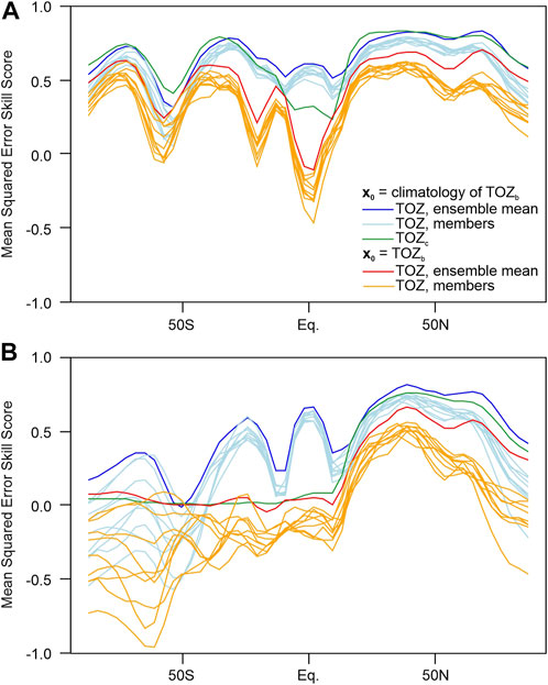
FIGURE 4. Results of the evaluation in terms of the MSESS (A), full network (B), and sparse network mimicking 1942, with seven stations, all in the Northern Hemisphere).

The same analysis for the sparse network (Figure 4B) shows a similar skill in the northern subtropics and mid-latitudes. It seems that the seven available stations are sufficient for this region. Skill deteriorates towards the poles and particularly in the Southern Hemisphere. The curve for TOZ_c is flat in the Southern Hemisphere, as is the curve for the ensemble mean when expressed against TOZ_b. Hence, there is no evidence from observations. There is still skill in TOZ in the tropics and in the southern subtropics (blue lines), but this comes entirely from the model forcings. This means that one should be careful in interpreting trends in the Southern Hemisphere. Overall, HISTOZ2 is useful for the analysis of interannual-to-long term variability in total column ozone, provided that the best use is made of the information contained in the different assimilation versions. The dataset is insufficient for analyzing the Southern Hemisphere prior to 1958 and for analyzing tropospheric ozone trends.

Next, I analyzed the resulting time series in TOZ and TOZ_c (Figure 5). Four latitude bands were chosen near locations where data are assimilated, namely, 75°N, 50°N, 20°N, and 38°S. All series were deseasonalized and filtered with a 28-month moving average. Note again that TOZ_b (black curve) and TOZ_c (blue curve) are independent. Figure 3 also shows strong inter-to-multiannual variability. In addition to the aforementioned spikes in the northern extratropics, we also see decreases in total column ozone in the tropics related to the volcanic eruptions of Pinatubo (1991), El Chichón (1982), and possibly Mt. Agung (1963). Over the 1924–1963 period, a slight upward trend is observed, which is analyzed in more detail in the following paragraphs. The figure also shows total column ozone from the NIWA dataset (TOZ_NIWA). There is an excellent agreement between the assimilated datasets and TOZ_NIWA at the three Northern Hemispheric latitudes (a good agreement is also found with the pure model simulations, TOZ_b), but the disagreement is visible in the southern extratropics (including with TOZ_b).

FIGURE 5

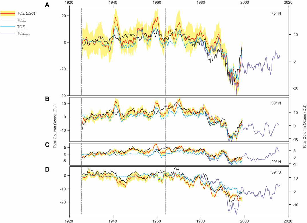
FIGURE 5. Time series of TOZ (including ±2 standard deviations), TOZ_c, TOZ_b (all on the left scales), and TOZ_NIWA (right y-axes) at latitudes of (A) 75° N, (B) 50° N, (C) 20° N, and (D) 39° S. The data were deseasonalized (based on the 1924–1974 period, in the case of TOZ, TOZ_c, and TOZ_b; based on 1979–2016, in the case of TOZ_NIWA) and then filtered with a 28-month moving average.

The data can also be visualized as Hovmöller plots (Figure 6). These data show the dominating interannual-to-multiannual variability in the northern extratropics and high latitudes, where observations are available. However, the visual analysis also reveals other details. For instance, TOZ shows a sign of the QBO, which is first absent in TOZ_c and only appears towards the end of the period in this dataset, when sufficient tropical stations are assimilated.

FIGURE 6

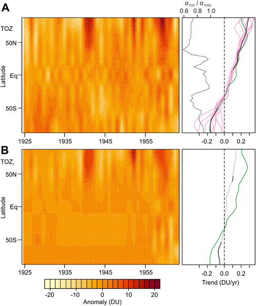
FIGURE 6. Anomalies of ensemble mean annual means of TOZ (A) and TOZ_c. (B) Right: linear trends per latitude for the corresponding datasets over the 1924–1963 period (non-significant (p = 0.05) in grey, significant in black, and individual members for TOZ in pink). Trends for TOZ_b are shown in green in both the panels. The dashed line in the upper right panel indicates the reduction in the ensemble spread of the trend in TOZ as compared to the prior TOZ_b.

The trends over the 1924–1963 period for each latitude (right insets) showed an increase in the Northern Hemisphere and a decrease in the Southern Hemisphere (although the latter has almost no data and should be interpreted with care). The sign and latitudinal pattern of the trend is similar in TOZ and TOZ_c, and the trends are in the range of −0.2 to 0.2 DU/year for TOZ and −0.1 to 0.1 DU/year for TOZ_c. It is to be noted that trends (except in the southern high latitudes and a tiny stretch in the Northern Hemisphere) are insignificant in TOZ_c. In TOZ, significant trends are found in the extratropics of both hemispheres. However, the significance only measures the trend line uncertainty and not the data uncertainty. For TOZ, I, therefore, also included the trends for each member, which shows that there is considerable scatter at mid-to-high latitudes.

Figure 6 also shows the trend in the pure model simulation (TOZ_b). The trend in TOZ is very close to that in TOZ_b. This can occur if the observations and models agree, or if the observations have hardly any impact in the assimilation. Here, the former is the case. This can be shown by the fact that the ensemble spread in TOZ is smaller than that in TOZ_b (dashed line in Figure 6, top right), with only 60% at mid-latitudes. Thus, assimilating observations brings the trends of the members closer to that of the mean. It can also be shown by the fact that TOZ_c, which is independent of TOZ_b, shows a similar pattern, which in that case is purely due to observations. The trend in TOZ_c is smaller than in TOZ as is expected from the fact that TOZ_c has a time-independent prior that does not see any forced trend and from the fact that observations are arguably too sparse and too segmented to reproduce the full trend.

A more detailed analysis of the trends as a function of latitude and month (Figure 7) shows that trends in the Northern Hemisphere are the largest from mid-winter to summer (i.e., they stretch across both seasons in the assimilation procedure). Trends in the Southern Hemisphere are the strongest and most significant in late austral winter and spring. However, the Hovmöller plot implies that the very low variance of TOZ_c in the Southern Hemisphere until around 1950 contributes to this result. The trend is affected strongly by the few observations at the end of the period.

FIGURE 7

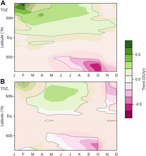
FIGURE 7. Trends in TOZ (A) and TOZ_c (B) over the 1924–1963 period as a function of latitude and month. Non-significant trends (p = 0.05) are shaded.

In order to focus more closely on the trend (which in TOZ_c is only marginally significant in Figures 6, 7), I used a regression approach to remove variability induced by atmospheric circulation variables, as well as by the 11-year solar cycle. The residuals were studied in the same way, i.e., as the Hovmöller plot and calculating a linear trend. Not all explanatory variables are statistically significant (p<0.1) at all latitudes, but each variable is significant at several latitudes and all variables are theoretically meaningful. Compared to individual locations (see Supplementary Figure S1), the regression for zonal averages has somewhat lower explained variances (Figure 8), ca. 20%–60%. Nevertheless, this helps reduce the dynamical part of the signal and obtains more robust trend estimates.

FIGURE 8

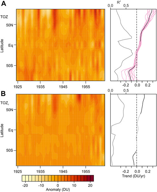
FIGURE 8. Residuals of the regression for TOZ (A) and TOZ_c. (B) Right: linear trends per latitude for the corresponding datasets over the 1924–1963 period (non-significant (p = 0.05) in grey, significant in black, and individual members for TOZ in pink). The dotted line in the right panels shows the explained variance of the regression model.

The Hovmöller diagrams of the residuals (Figure 8) show lower variability, but the regression does not fully explain all excursions. The QBO signature is weaker, and the three strong excursions and northern mid-to-high latitudes in the early 1940s, and the early and late 1950s are also weaker. Trends (right insets) of the residuals are almost identical to those found in the raw data, and their latitudinal pattern remains the same. However, they are more significant, particularly for TOZ_c.

Finally, I also analyzed the vertical structure of the ozone trend in the 2D version of the assimilated datasets. Note that none of the observations used in this study provides a vertical profile. Therefore, the vertical trend structure comes from the prior (i.e., the raw model simulations) or from the assimilation through the covariance matrix. The trend in the ozone number density as a function of latitude and altitude (Figure 9) shows that the decreasing trend in the southern high latitudes originates in the lower stratosphere and is the strongest in September and October (Figure 7).

FIGURE 9

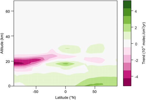
FIGURE 9. Trend on the ozone number density in annual mean ozone in the assimilated dataset (HISTOZv2) from 1924 to 1963.

The positive trend in the Northern Hemisphere is the strongest in winter, spring, and summer (Figure 7), and its vertical structure shows increases in the troposphere around 50°N and to a lesser extent in the lowermost stratosphere from the tropics to the northern polar region. Small positive trends are also found in the Southern Hemisphere’s troposphere.

4 Discussion

This study compiled and digitized as much of the historical total column observations as possible and used data assimilation to assess variability and trends in the period 1924–1963. Uncertainties in the observations are likely large. Nevertheless, a consistent picture emerges from all analyses conducted. The analysis of the raw data does not show a preference for positive or negative trends, although trend magnitudes in individual segments may be relatively large due to their short length.

Assimilating the segments into a numerical model provides several datasets of total column ozone as a function of latitude and time, as well as 2D data on the ozone number density. The datasets are not only an update to HISTOZ (using more observations and an improved assimilation scheme) but also provide a new product, such as an assimilation using a time-invariant prior. This allows addressing the role of observations and of the forced model simulations on the product. Furthermore, as all products are ensembles, a measure of uncertainty of the procedure is available.

The evaluation of the products indicates a generally high skill for TOZ (Figure 4), which is due to both the forced model runs and the observations. Experiments assessing different networks show that for the historical period, only the Northern Hemisphere has more skill than the forced simulations alone, and hence, any interpretation of the Southern Hemisphere trends will strongly be affected by the model (Figure 4). At the same time, the evaluation shows that even the network of the 1940s is dense enough to provide information on total column ozone at northern mid-latitudes. The evaluations also show that the SOCOL simulations fit well with the observations from ground-based stations, as well as satellite data (Figure 5).

The products, first of all, point to large interannual-to-multiannual variability in the period 1924–1963. El Niño/Southern Oscillation is an important source of this variability (see Domeisen et al., 2019). Concerning the interpretation of trends, it should again be noted that the individual series carry large uncertainties. Therefore, I tried to assess and minimize their effects as far as possible. The homogenized series do not show obvious step changes. The other series were segmented at instances of known changes to the station or the instrument or long gaps. Segments are then debiased individually, which can be considered a form of homogenization. The shorter the segments get, however, the smaller the trend signal they retain. Hence, they underestimate trends by construction. Furthermore, errors and uncertainties are addressed at the level of the input data (assigned error variance), the assimilation (ensemble spread and its reduction), the different products generated (TOZ_b, TOZ, and TOZ_c), the statistical procedure (explained variance of the regression model), and trend estimations. Taken together, this allows a more robust picture of trends in the pre-CFC era than hitherto possible.

The interpretation of trends relies on, and is plausibilized by, analyzing the differences between TOZ and TOZ_c (and contrasting them with TOZ_b), the latitudinal pattern, the seasonal pattern, and the vertical pattern. Together, this indicates that the negative trends in the southern high latitudes are due to changes in the lower stratosphere in austral spring (due to ozone depletion in the very last years of the 40-year period). This result might be affected by the lack of observations in the southern mid-to-high latitudes prior to the 1950s but is in agreement with CMIP6 models (Keeble et al., 2021; Zeng et al., 2022).

The positive trends in the northern mid- and high-latitudes are the strongest in winter, spring, and summer, not only in the troposphere but also in the lower stratosphere. The tropospheric signal might be due to tropospheric ozone production or transport. In SOCOL, tropospheric chemistry is rudimentary and consists only of the oxidation of CO and methane, which may not be sufficient to capture tropospheric ozone trends. In CMIP6 models, tropospheric ozone increases rather strongly after ca. 1950, driven by increasing emissions of NOx and other precursors (Griffiths et al., 2021). However, sparse information on surface ozone over this period from measurements (Tarasick et al., 2019) indicates that the main increase between historical conditions and the present day at northern mid-latitudes occurred after 1963. No observation-based statement can be made on the tropospheric ozone column. In addition to a tropospheric signal in spring and summer, the analysis also shows a signal in the lower stratosphere in winter and spring that cannot be explained by tropospheric chemistry.

Changes in atmospheric dynamics might contribute to trends. Although the regression model was designed to reduce their effect, there is still a remaining dynamically induced variability in the record. For instance, the northern tropical belt moved equatorward from the mid-1940s to mid-1970s (Brönnimann et al., 2015). If this trend already started in the 1920s, a positive trend at northern mid-latitudes might result.

The latitudinal structure of the trends found in this study fits well with CMIP6 models (Keeble et al., 2021; Zeng et al., 2022). However, the magnitudes differ. For the 30°–60° N band, I find trends of 0.19 and 0.09 DU/year in TOZ and TOZ_c, respectively. The corresponding trends for the residuals are even smaller, 0.14 and 0.08 DU/year. Taking the TOZ trend of the residual as the representative, one would expect a change of 6 DU over the entire period, which is around half the change in Keeble et al. (2021). Egorova et al. (2020) found a similarly large change over the 1910–1940 period. Zeng et al. (2022), in CMIP6 models, found an increase of ca. 10 DU for the 30°–60°N band in the annual mean, of which ca. 6 DU occurs in the tropospheric column and 4 DU in the stratospheric column. The trend is mostly due to the near-term climate forcers (troposphere) and methane (both troposphere and stratosphere). All of this is consistent with my findings. Given the large uncertainties, also the amplitudes might still be consistent over the 1924–1963 period. However, in CMIP6, total column ozone at 30°–60°N in 1924 is lower than at the period of maximum ozone depletion in the late 1990s, for which there is no evidence in the observations, and this trend extends further backward.

5 Conclusion

In this paper, I analyze the evolution of total column ozone in the pre-CFC era, from 1924 to 1963. Although the observations remain sparse, compiling (and rescuing) as much of them as possible and using a data assimilation approach, nevertheless, allow a glimpse at variability and trends in total column ozone in this period at the global level. This approach allows incorporating uncertainties in different ways: specifically (as observation errors), by segmenting the series, by comparing different assumptions (priors), by analyzing an ensemble and its spread, and eventually by analyzing uncertainties in the statistical analyses. Furthermore, by analyzing latitudinal, season, and vertical patterns, a robust picture emerges.

Results show that interannual-to-multiannual variations in zonal mean total column ozone were large in the 1924–1963 period, whereas trends were relatively small both before and after accounting for dynamically induced variability in a regression approach. Total column ozone increased over the northern extratropics in winter, spring, and summer due to both changes in the tropospheric and lower stratospheric ozone. At the southern mid-to-high latitudes, total column ozone decreased in austral spring in the lowermost stratosphere and due to ozone depletion at the very end of the period, although there are very few observations to constrain this.

This latitudinal trend pattern fits well with that in CMIP6 model simulations. However, over the 30°–60° N latitude band, which is the one best constrained by observations and has the strongest observed trend, models produce a considerably larger trend. These trends point to the need for further evaluation of both observations and simulations and the need for better understanding of the potential reasons for the inconsistency in the mid-latitude total column ozone trends over the mid-20th century.

Data availability statement

The input data and the code to generate the HISOZ2 ozone data sets can be found at: https://doi.org/10.6084/m9.figshare.21387468.v1. The HISTOZ2 data sets can be downloaded here: https://boris-portal.unibe.ch/handle/20.500.12422/208.

Author contributions

SB conceived the study, digitized, and compiled the data, performed the analysis, and wrote the paper.

Funding

This work was supported by the European Commission (ERC Grant PALAEO-RA, 787574).

Acknowledgments

The author would like to thank Alkis Bais for sending the scans of historical data sheets.

Conflict of interest

The author declares that the research was conducted in the absence of any commercial or financial relationships that could be construed as a potential conflict of interest.

Publisher’s note

All claims expressed in this article are solely those of the authors and do not necessarily represent those of their affiliated organizations, or those of the publisher, the editors, and the reviewers. Any product that may be evaluated in this article, or claim that may be made by its manufacturer, is not guaranteed or endorsed by the publisher.

Supplementary material

The Supplementary Material for this article can be found online at: https://www.frontiersin.org/articles/10.3389/feart.2023.1079510/full#supplementary-material

References

Angione, R. J., and Roosen, R. G. (1983). Baseline ozone results from 1923 to 1955. J. Clim. Appl. Meteorol. 22, 1377–1383. doi:10.1175/1520-0450(1983)022<1377:borft>2.0.co;2

CrossRef Full Text | Google Scholar

Ball, W. T., Chiodo, G., Abalos, M., Alsing, J., and Stenke, A. (2020). Inconsistencies between chemistry–climate models and observed lower stratospheric ozone trends since 1998. Atmos. Chem. Phys. 20, 9737–9752. doi:10.5194/acp-20-9737-2020

CrossRef Full Text | Google Scholar

Bodeker, G. E., Nitzbon, J., Tradowsky, J. S., Kremser, S., Schwertheim, A., and Lewis, J. (2021). A global total column ozone climate data record. Earth Syst. Sci. Data 13, 3885–3906. doi:10.5194/essd-13-3885-2021

CrossRef Full Text | Google Scholar

Bognar, K., Tegtmeier, S., Bourassa, A., Roth, C., Warnock, T., Zawada, D., et al. (2022). Stratospheric ozone trends for 1984–2021 in the SAGE II–OSIRIS–SAGE III/ISS composite dataset. Atmos. Chem. Phys. 22, 9553–9569. doi:10.5194/acp-22-9553-2022

CrossRef Full Text | Google Scholar

Brönnimann, S., Annis, J. L., Vogler, C., and Jones, P. D. (2007). Reconstructing the quasi-biennial oscillation back to the early 1900s. Geophys. Res. Lett. 34, L22805. doi:10.1029/2007gl031354

CrossRef Full Text | Google Scholar

Brönnimann, S., Bhend, J., Franke, J., Fluckiger, S., Fischer, A. M., Bleisch, R., et al. (2013). A global historical ozone data set and prominent features of stratospheric variability prior to 1979. Atmos. Chem. Phys. 13, 9623–9639. doi:10.5194/acp-13-9623-2013

CrossRef Full Text | Google Scholar

Brönnimann, S. (2022). Century-long column ozone records show that chemical and dynamical influences counteract each other. Commun. Earth Environ. 3, 143. doi:10.1038/s43247-022-00472-z

CrossRef Full Text | Google Scholar

Brönnimann, S., Fischer, A. M., Rozanov, E., Poli, P., Compo, G. P., and Sardeshmukh, P. D. (2015). Southward shift of the Northern tropical belt from 1945 to 1980. Nat. Geosci. 8, 969–974. doi:10.1038/ngeo2568

CrossRef Full Text | Google Scholar

Brönnimann, S., Luterbacher, J., Staehelin, J., Svendby, T. M., Hansen, G., and Svenøe, T. (2004). Extreme climate of the global troposphere and stratosphere in 1940-42 related to El Niño. Nature 431, 971–974. doi:10.1038/nature02982

PubMed Abstract | CrossRef Full Text | Google Scholar

Brönnimann, S., and Nichol, S. (2020). Total column ozone in New Zealand and in the UK in the 1950s. Atmos. Chem. Phys. 20, 14333–14346. doi:10.5194/acp-20-14333-2020

CrossRef Full Text | Google Scholar

Brönnimann, S., Staehelin, J., Farmer, S. F. G., Cain, J. C., Svendby, T. M., and Svenøe, T. (2003). Total ozone observations prior to the IGY. I: A history. Q. J. Roy. Meteorol. Soc. 129, 2797–2817. doi:10.1256/qj.02.118

CrossRef Full Text | Google Scholar

De Muer, D., and De Backer, H. (1992). Revision of 20 years of Dobson total ozone data at Uccle (Belgium): Fictitious Dobson total ozone trends induced by sulfur dioxide trends. J. Geophys. Res. 97, 5921–5937. doi:10.1029/91jd03164

CrossRef Full Text | Google Scholar

Dietmüller, S., Garny, H., Eichinger, R., and Ball, W. T. (2021). Analysis of recent lower-stratospheric ozone trends in chemistry climate models. Atmos. Chem. Phys. 21, 6811–6837. doi:10.5194/acp-21-6811-2021

CrossRef Full Text | Google Scholar

Dobson, G. M. B., and Harrison, D. N. (1926). Measurements of the amount of ozone in the Earth’s atmosphere and its relation to other geophysical conditions. Proc. Roy. Soc. Lond. A110, 660–693.

Google Scholar

Domeisen, D. I., Garfinkel, C. I., and Butler, A. H. (2019). The teleconnection of El Niño southern oscillation to the stratosphere. Rev. Geophys. 57, 5–47. doi:10.1029/2018rg000596

CrossRef Full Text | Google Scholar

Egorova, T., Rozanov, E., Arsenovic, P., and Sukhodolov, T. (2020). Ozone layer evolution in the early 20th century. Atmosphere 11 (2), 169. doi:10.3390/atmos11020169

CrossRef Full Text | Google Scholar

Fischer, A. M., Schraner, M., Rozanov, E., Kenzelmann, P., Schnadt Poberaj, C., Brunner, D., et al. (2008). Interannual-to-Decadal variability of the stratosphere during the 20th century: Ensemble simulations with a chemistry-climate model. Atmos. Chem. Phys. 8, 7755–7777. doi:10.5194/acp-8-7755-2008

CrossRef Full Text | Google Scholar

Griffiths, P. T., Murray, L. T., Zeng, G., Shin, Y. M., Abraham, N. L., Archibald, A. T., et al. (2021). Tropospheric ozone in CMIP6 simulations. Atmos. Chem. Phys. 21, 4187–4218. doi:10.5194/acp-21-4187-2021

CrossRef Full Text | Google Scholar

Hansen, G., and Svenøe, T. (2005). Multilinear regression analysis of the 65-year Tromsø total ozone series. J. Geophys. Res. 110, D10103. doi:10.1029/2004jd005387

CrossRef Full Text | Google Scholar

Keeble, J., Hassler, B., Banerjee, A., Checa-Garcia, R., Chiodo, G., Davis, S., et al. (2021). Evaluating stratospheric ozone and water vapour changes in CMIP6 models from 1850 to 2100. Atmos. Chem. Phys. 21, 5015–5061. doi:10.5194/acp-21-5015-2021

CrossRef Full Text | Google Scholar

Komhyr, W., Barrett, E., Slocum, G., and Weickmann, H. K. (1971). Physical sciences: Atmospheric total ozone increase during the 1960s. Nature 232, 390–391. doi:10.1038/232390a0

PubMed Abstract | CrossRef Full Text | Google Scholar

Lean, J. L. (2018). Estimating solar irradiance since 850 CE. Earth Space Sci. 5, 133–149. doi:10.1002/2017ea000357

CrossRef Full Text | Google Scholar

Orbe, C., Wargan, K., Pawson, S., and Oman, L. D. (2020). Mechanisms linked to recent ozone decreases in the Northern Hemisphere lower stratosphere. J. Geophys. Res.-Atmos. 125, e2019JD031631. doi:10.1029/2019jd031631

CrossRef Full Text | Google Scholar

SPARC/IO3C/GAW (2019). “Report on long-term ozone trends and uncertainties in the stratosphere (LOTUS),” in SPARC report No. 9, GAW report No. 241, WCRP-17/2018. Editors I. Petropavlovskikh, S. Godin-Beekmann, D. Hubert, R. Damadeo, B. Hassler, and V Sofieva.

Google Scholar

Schraner, M., Rozanov, E., Schnadt Poberaj, C., Kenzelmann, P., Fischer, A. M., Zubov, V., et al. (2008). Technical note: Chemistry-climate model SOCOL: Version 2.0 with improved transport and chemistry/microphysics schemes. Atmos. Chem. Phys. 8, 5957–5974. doi:10.5194/acp-8-5957-2008

CrossRef Full Text | Google Scholar

Shindell, D. T., and Faluvegi, G. (2002). An exploration of ozone changes and their radiative forcing prior to the chlorofluorocarbon era. Atmos. Chem. Phys. 2, 363–374. doi:10.5194/acp-2-363-2002

CrossRef Full Text | Google Scholar

Slivinski, L. C., Compo, G. P., Whitaker, J. S., Sardeshmukh, P. D., Giese, B. S., McColl, C., et al. (2019). Towards a more reliable historical reanalysis: Improvements for version 3 of the Twentieth Century Reanalysis system. Q. J. Roy. Meteorol. Soc. 145, 2876–2908. doi:10.1002/qj.3598

CrossRef Full Text | Google Scholar

Solomon, S., Ivy, D. J., Kinnison, D., Mills, M. J., Neely, R. R., and Schmidt, A. (2016). Emergence of healing in the Antarctic ozone layer. Science 353, 269–274. doi:10.1126/science.aae0061

PubMed Abstract | CrossRef Full Text | Google Scholar

Solomon, S. (1999). Stratospheric ozone depletion: A review of concepts and history. Rev. Geophys. 37, 275–316. doi:10.1029/1999rg900008

CrossRef Full Text | Google Scholar

Staehelin, J., Renaud, A., Bader, J., McPeters, R., Viatte, P., Hoegger, B., et al. (1998). Total ozone series at Arosa (Switzerland): Homogenization and data comparison. J. Geophys. Res. 103, 5827–5841. doi:10.1029/97jd02402

CrossRef Full Text | Google Scholar

Steinbrecht, W., Hegglin, M. I., Harris, N., and Weber, M. (2018). Is global ozone recovering? Comptes Rendus Geosci. 350, 368–375. doi:10.1016/j.crte.2018.07.012

CrossRef Full Text | Google Scholar

Tarasick, D., Galbally, I. E., Cooper, O. R., Schultz, M. G., Ancellet, G., Leblanc, T., et al. (2019). Tropospheric Ozone Assessment Report: Tropospheric ozone from 1877 to 2016, observed levels, trends and uncertainties. Elem. Sci. Anth 7, 39. doi:10.1525/elementa.376

CrossRef Full Text | Google Scholar

Valler, V., Franke, J., Brugnara, Y., and Brönnimann, S. (2022). An updated global atmospheric paleo-reanalysis covering the last 400 years. Geosc Data J. 9, 89–107. doi:10.1002/gdj3.121

CrossRef Full Text | Google Scholar

Weber, M., Arosio, C., Coldewey-Egbers, M., Fioletov, V. E., Frith, S. M., Wild, J. D., et al. (2022). Global total ozone recovery trends attributed to ozone-depleting substance (ODS) changes derived from five merged ozone datasets. Atmos. Chem. Phys. 22, 6843–6859. doi:10.5194/acp-22-6843-2022

CrossRef Full Text | Google Scholar

WMO (World Meteorological Organization) (2018). Scientific assessment of ozone depletion: 2018. Geneva, Switzerland, 588. Global Ozone Research and Monitoring Project – Report No. 58.

Google Scholar

Zeng, G., Morgenstern, O., Williams, J. H. T., O’Connor, F. M., Griffiths, P. T., Keeble, J., et al. (2022). Attribution of stratospheric and tropospheric ozone changes between 1850 and 2014 in CMIP6 models. J. Geophys. Res. 127, e2022JD036452. doi:10.1029/2022jd036452

CrossRef Full Text | Google Scholar

Ziemke, J. R., Labow, G. J., Kramarova, N. A., McPeters, R. D., Bhartia, P. K., Oman, L. D., et al. (2021). A global ozone profile climatology for satellite retrieval algorithms based on Aura MLS measurements and the MERRA-2 GMI simulation. Atmos. Meas. Tech. 14, 6407–6418. doi:10.5194/amt-14-6407-2021

CrossRef Full Text | Google Scholar