Probabilistic approach to Gramian inversion of multiphysics data

1 Introduction

Different geophysical methods provide information about various physical properties of rock formations and mineralization. In many cases, this information is mutually complementary. At the same time, inversion of the data for a particular survey is subject to considerable uncertainty and ambiguity as to causative body geometry and intrinsic physical property contrast. One productive approach to reducing uncertainty is to jointly invert several types of data. In the framework of joint inversion, the goal is to fit different types of predicted data to the corresponding observed data while keeping specific relationships between the different physical properties of the rocks. This can be achieved by using the known petrophysical relationships between different physical properties of the rocks within the framework of the inversion process (Afnimar et al., 2002; Hoversten et al., 2006; Moorkamp et al., 2011; Gao et al., 2012; Zhdanov, 2015; Moorkamp et al., 2016; Giraud et al., 2017; Giraud et al., 2019).

The alternative approach is based on using the Gramian constraints introduced in (Zhdanov et al., 2012a; Zhdanov et al., 2012b). The advantage of Gramian constraints is that they enforce the functional relationships between different physical parameters without a priori knowledge of the specific form of these relationships. In the original publications (Zhdanov et al., 2012a; Zhdanov et al., 2012b; Zhdanov, 2015), the Gramian constraints were introduced in the framework of the deterministic approach to the solution of the inverse problem, which considers the data and model parameters characterized by specific functions or vectors with certain (maybe unknown) values. However, there is a probabilistic approach to inverse problems where the observed data and model parameters are treated as realizations of some random variables. This approach was introduced in the pioneering papers of (Foster, 1961), (Franklin, 1970), (Jackson, 1972), (Tarantola and Valette, 1982), and (Tarantola, 1987; Tarantola, 2005).

It can be demonstrated that both these approaches result in similar numerical solutions of the inverse problem (Zhdanov, 2002). At the same time, deterministic or probabilistic interpretation of the observed data and model parameters emphasize different aspects of the inversion algorithms. This also helps understand better the properties of the inversion parameters.

This paper introduces a novel approach to the joint inversion where the Gramian constraints are represented in the probabilistic form as the determinant of the covariance matrix between the different model parameters.

2 Gramian constraints

Gramian constraints enforce the correlation between different parameters and their transforms or attributes (Zhdanov et al., 2012a; Zhdanov, 2015). By imposing the requirement of the minimum of the Gramian mathematical operator in regularized inversion, we obtain multi-modal inverse solutions with enhanced correlations between the different model parameters or their attributes.

Let us consider forward geophysical problems for multiple geophysical data sets. These problems can be described by the following operator relationships:

$d^{\left(i\right)}=A^{\left(i\right)}\left(m^{\left(i\right)}\right),i=\mathrm{1,2,3},\dots ,n;(1)$

where, in a general case, A⁽ⁱ⁾ is a non-linear operator, d⁽ⁱ⁾ $\left(i=\mathrm{1,2,3},\dots ,n\right)$ are different observed data sets (which may have different physical natures and/or parameters), and $m^{(i)}\left(i=\mathrm{1,2,3},\dots ,n\right)$ are the unknown sets of model parameters.

Note that, diverse model parameters may have different physical dimensions (e.g., density is measured in g/cm³, resistivity is measured in Ohm-m, etc.).

It is convenient to introduce the dimensionless weighted model parameters, ${\tilde{m}}^{(i)}$, defined as follows:

${\tilde{m}}^{\left(i\right)}=W_m^{\left(i\right)}{m}^{\left(i\right)},(2)$

where $W_m^{(i)}$ is the corresponding linear operator of the model weighting (Zhdanov, 2002; Zhdanov, 2015).

Note that, in the following sections of the paper we will omit “wave” above the symbols of the model parameters to simplify the notations. However, we always assume that we work with the dimensionless model parameters.

These parameters can be described by integrable functions of a radius-vector $\mathbf{r}=\left(x,y,z\right)$ defined within some volume V of a 3D space. The set of these functions forms a complex, in a general case, Hilbert space of the model parameters, M, with a L₂ norm, defined by the corresponding inner product:

$\begin{array}{ll}\hfill {\left(m^{\left(i\right)},m^{\left(j\right)}\right)}_M& ={\iiint }_V{m}^{\left(i\right)}\left(\mathbf{r}\right)\cdot m^{\left(j\right)*}\left(\mathbf{r}\right)dv,\hfill \\ \hfill {‖m^{\left(i\right)}‖}_M^2& ={\left(m^{\left(i\right)},m^{\left(i\right)}\right)}_M,\hfill \end{array}(3)$

where asterisk “*” denotes the complex conjugate value.

Similarly, different data, as a rule, have distinct physical dimensions as well. Therefore, it is convenient to consider dimensionless weighted data, ${\tilde{d}}^{(i)}$, defined as follows:

${\tilde{d}}^{\left(i\right)}=W_d^{\left(i\right)}{d}^{\left(i\right)},(4)$

where $W_d^{(i)}$ is the corresponding linear operator of data weighting. However, to simplify the notations, we will drop the “wave” above the symbols of the data, assuming nevertheless that the data are dimensionless.

The selection of the model and data weights was discussed in many publications on inversion theory. For example, in the framework of the probabilistic approach (Tarantola, 1987), the weights are determined as inverse data covariance or model covariance matrices. In the framework of the deterministic approach (Zhdanov, 2002, 2015), the weights are determined as inverse integrated sensitivity matrices.

We also assume that the data belong to some complex Hilbert space of the data, D, with the L₂ norm, defined by the corresponding inner product:

$\begin{array}{ll}\hfill {\left(d^{\left(i\right)},d^{\left(j\right)}\right)}_D& ={\iint }_S{d}^{\left(i\right)}\left(\mathbf{r}\right)d^{\left(j\right)*}\left(\mathbf{r}\right)ds,\hfill \\ \hfill {‖d^{\left(i\right)}‖}_D^2& ={\left(d^{\left(i\right)},d^{\left(i\right)}\right)}_D,\hfill \end{array}(5)$

where S is an observation surface.

Joint inversion of multiphysics data can be reduced to minimization of the following parametric functional,

$\begin{array}{ll}\hfill P_G^{\alpha }\left(m^{\left(1\right)},m^{\left(2\right)},\dots .,m^{\left(n\right)}\right)=& \sum _{i=1}^n\phi \left(m^{\left(i\right)}\right)\hfill \\ \hfill & +\alpha S_G\left(m^{\left(1\right)},m^{\left(2\right)},\dots .,m^{\left(n\right)}\right),\hfill \end{array}(6)$

where α ∈ [0, ∞) is the regularization parameter.

Misfit functionals, $\phi \left(m^{(i)}\right)$, are defined as follows,

$\phi \left(m^{\left(i\right)}\right)=\Vert A^{\left(i\right)}\left(m^{\left(i\right)}\right)-d^{\left(i\right)}{\Vert }_D^2;(7)$

where A⁽ⁱ⁾(m⁽ⁱ⁾) are the predicted data,

The term S_G(m⁽¹⁾, m⁽²⁾, …. m⁽ⁿ⁾) is the constraint stabilizing functional. This functional can be introduced as a determinant of the Gram matrix of a system of model parameters, m⁽¹⁾, m⁽²⁾, …. m⁽ⁿ⁾, which is called a Gramian (Zhdanov et al., 2012a; Zhdanov, 2015):

$\begin{array}{ll}\hfill S_G& =G\left(m^{\left(1\right)},m^{\left(2\right)},\dots .,m^{\left(n\right)}\right)\hfill \\ \hfill & =\left|\begin{array}{cccc}\hfill \left(m^{\left(1\right)},m^{\left(1\right)}\right)\hfill & \hfill \left(m^{\left(1\right)},m^{\left(2\right)}\right)\hfill & \hfill \dots \hfill & \hfill \left(m^{\left(1\right)},m^{\left(n\right)}\right)\hfill \\ \hfill \left(m^{\left(2\right)},m^{\left(1\right)}\right)\hfill & \hfill \left(m^{\left(2\right)},m^{\left(2\right)}\right)\hfill & \hfill \dots \hfill & \hfill \left(m^{\left(2\right)},m^{\left(n\right)}\right)\hfill \\ \hfill \dots \hfill & \hfill \dots \hfill & \hfill \dots \hfill & \hfill \dots \hfill \\ \hfill \left(m^{\left(n\right)},m^{\left(1\right)}\right)\hfill & \hfill \left(m^{\left(n\right)},m^{\left(2\right)}\right)\hfill & \hfill \dots \hfill & \hfill \left(m^{\left(n\right)},m^{\left(n\right)}\right)\hfill \end{array}\right|,\hfill \end{array}(8)$

where (-,-) stands for the inner product in the corresponding Hilbert space of model parameters, defined by Eq. 3.

Note that, in case of discrete model parameters, expression (3) for inner product takes the following form:

$\left(m^{\left(i\right)},m^{\left(j\right)}\right)=\sum _{l=1}^L{m}_l^{\left(i\right)}{m}_l^{\left(j\right)*},(9)$

where $m_l^{(i)}$ are the discrete values of the corresponding parameter; L is the total number of every discretized model parameter within the modeling domain V, assuming that we use the same discretization for all parameters.

The main property of the Gramian (Eq. 8) is that it is a non-negative functional, (e.g., Everitt, 1958; Barth, 1999):

$G\left(m^{\left(1\right)},m^{\left(2\right)},\dots .,m^{\left(n\right)}\right)\ge 0.(10)$

The equality holds in (Eq. 10) if the system of functions $\left(m^{(1)},m^{(2)},\dots .,m^{(n)}\right)$ is linearly dependent.

It was demonstrated in (Zhdanov et al., 2012a) and (Zhdanov, 2015) that one could apply the Gramian constraints to different transforms of the model parameters. For example, we may consider differential operations, like gradient, applied to the spatial distribution of the model parameters. This will result in the shared Earth model characterized by similar behavior of the gradients of different physical properties. In this case, Gramian constraint, similarly to the cross-gradient method (Gallardo and Meju, 2003, 2004, 2007, 2011; Gallardo, 2007), enforces the structural similarity between different physical inverse models (Zhdanov et al., 2021). We can also use various functions of the model parameters, e.g., logarithms or trigonometric functions, to enforce the correlation between the transformed parameters.

3 Covariance representation of the probabilistic Gramian stabilizer

In the framework of the probabilistic approach to the solution of the inverse problem, we consider the observed data and the model parameters as realizations of some random variables. The joint inversion requires the enforcement of some relations between different model parameters, which can be achieved by adding the term containing the covariance matrix between different model parameters, which serves as an analog of Gramian in a deterministic approach (Zhdanov et al., 2012a).

The probabilistic Gramian stabilizer, $S_{G_{\sigma }},$can be introduced as the determinant of the covariance matrix between different model parameters in a probabilistic approach to the inversion theory:

$\begin{array}{ll}\hfill S_{G_{\sigma }}& \left(m^{\left(1\right)},m^{\left(2\right)},\dots .m^{\left(n\right)}\right)=\text{det}\left({\sigma }_n\right)\hfill \\ \hfill & =\left|\begin{array}{cccc}\hfill cov\left(m^{\left(1\right)},m^{\left(1\right)}\right)\hfill & \hfill \dots \hfill & \hfill cov\left(m^{\left(1\right)},m^{\left(n-1\right)}\right)\hfill & \hfill cov\left(m^{\left(1\right)},m^{\left(n\right)}\right)\hfill \\ \hfill cov\left(m^{\left(2\right)},m^{\left(1\right)}\right)\hfill & \hfill \dots \hfill & \hfill cov\left(m^{\left(2\right)},m^{\left(n-1\right)}\right)\hfill & \hfill cov\left(m^{\left(2\right)},m^{\left(n\right)}\right)\hfill \\ \hfill \dots \hfill & \hfill \dots \hfill & \hfill \dots \hfill & \hfill \dots \hfill \\ \hfill cov\left(m^{\left(n-1\right)},m^{\left(1\right)}\right)\hfill & \hfill \dots \hfill & \hfill cov\left(m^{\left(n-1\right)},m^{\left(n-1\right)}\right)\hfill & \hfill cov\left(m^{\left(n-1\right)},m^{\left(n\right)}\right)\hfill \\ \hfill cov\left(m^{\left(n\right)},m^{\left(1\right)}\right)\hfill & \hfill \dots \hfill & \hfill cov\left(m^{\left(n\right)},m^{\left(n-1\right)}\right)\hfill & \hfill cov\left(m^{\left(n\right)},m^{\left(n\right)}\right)\hfill \end{array}\right|.\hfill \end{array}(11)$

It is well known that the determinant of the covariance matrix is always non-negative, and it is equal to zero if and only if the random variables, $m^{(1)},m^{(2)},\dots ,m^{\left(n\right)}$, are linearly dependent (e.g., Ross, 2010). This property of the probabilistic Gramian is similar to that of the deterministic Gramian defined by Eq. 8. The key difference is in the way how we treat the model parameters. In the framework of the deterministic approach, they are described by specific (though unknown) functions. In the framework of the probabilistic approach, the model parameters are the realizations of some unknown random variables.

We should note also that the direct analogy between Eqs. 8 and 11 holds when the random model parameters have zero mean values. Indeed, in the case of discrete and real model parameters, the statistical estimate of the covariance is as follows:

$cov\left(m^{\left(i\right)},m^{\left(j\right)}\right)=\frac{1}{L-1}\sum _{l=1}^L\left(m_l^{\left(i\right)}-\langle m^{\left(i\right)}\rangle \right)\left(m_l^{\left(j\right)}-\langle m^{\left(j\right)}\rangle \right),(12)$

where ⟨⋅⟩ indicates the mean. If the mean values are zero, ⟨m^(i,j)⟩ = 0, then according to Eq. 9, we have

$cov\left(m^{\left(i\right)},m^{\left(j\right)}\right)=\frac{1}{L-1}\sum _{l=1}^L{m}_l^{\left(i\right)}{m}_l^{\left(j\right)}=\frac{1}{L-1}\left(m^{\left(i\right)},m^{\left(j\right)}\right).(13)$

In Supplementary Appendix S1 we discuss the Gramian space of random variables. One of the important properties of this space is that the distance between two variables is determined by the corresponding Gramian.

Let us consider the Gramian space Γ⁽ⁿ⁾ of random variables, representing model parameters with the core elements formed by model parameters m⁽¹⁾, m⁽²⁾, …, m⁽ⁿ⁻¹⁾. Then according to definition of norm in this space, equations S1 and S8 in the Supplementary Appendix we can write probabilistic Gramian as the norm of parameter m⁽ⁿ⁾:

$S_{G_{\sigma }}\left(m^{\left(1\right)},m^{\left(2\right)},\dots .m^{\left(n\right)}\right)={‖m^{\left(n\right)}‖}_{{\mathrm{\Gamma }}^{\left(n\right)}}^2.(14)$

We will use this property in formulating the principles of joint inversion using the probabilistic Gramian.

4 Regularization of the inverse problem using probabilistic Gramian

Following the general principles of regularization theory, we can now introduce a probabilistic parametric functional, $P_{\sigma }^{\alpha }$ as a linear combination of combined misfit functional, $\sum _{i=1}^n\phi \left(m^{(i)}\right)$, and probabilistic Gramian:

$\begin{array}{ll}\hfill P_{\sigma }^{\alpha }\left(m^{\left(1\right)},m^{\left(2\right)},\dots ,m^{\left(n\right)}\right)& =\sum _{i=1}^n\phi \left(m^{\left(i\right)}\right)\hfill \\ \hfill & +\alpha S_{G_{\sigma }}\left(m^{\left(1\right)},m^{\left(2\right)},\dots .m^{\left(n\right)}\right)\hfill \\ \hfill & =\min ,\hfill \end{array}(15)$

where α ∈ [0, ∞) is regularization parameter.

We should note that the parametric functional is similar to Eq. 6 if the joint stabilizing functional, S_G, is selected equal to the probabilistic Gramian, $S_{G_{\sigma }}$.

There exist several standard gradient type methods which can be used to solve the minimization problem—steepest descent, Newton, and conjugate gradient methods, for example,. All of them require calculation of the steepest ascent direction (gradient) of the corresponding functional. In the following section we will consider this problem in details.

4.1 Steepest ascent direction of the probabilistic parametric functional

The first variation of the parametric functional, $P_{\sigma }^{\alpha }$, with the probabilistic Gramian stabilizer can be calculated as follows:

$\begin{array}{ll}\hfill \delta P_{\sigma }^{\alpha }& \left(m^{\left(1\right)},m^{\left(2\right)},\dots ,m^{\left(n\right)}\right)\hfill \\ \hfill & =2\sum _{i=1}^n{\left(\delta A^{\left(i\right)}\left(m^{\left(i\right)}\right),A^{\left(i\right)}\left(m^{\left(i\right)}\right)-d^{\left(i\right)}\right)}_{{\mathrm{\Gamma }}_D^{\left(1\right)}}\hfill \\ \hfill & +\alpha \delta S_{G_{\sigma }}\left(m^{\left(1\right)},m^{\left(2\right)},\dots .m^{\left(n\right)}\right),\hfill \end{array}(16)$

where ${\mathrm{\Gamma }}_D^{\left(1\right)}$ is the probabilistic Gramian space of data with inner product defined by covariance according to formula S12 in the Supplementary Appendix.

The variation of the probabilistic Gramian stabilizer, according to Eq. 14, can be expressed as follows:

$\begin{array}{ll}\hfill \delta S_{G_{\sigma }}& \left(m^{\left(1\right)},m^{\left(2\right)},\dots .m^{\left(n\right)}\right)=\delta {‖m^{\left(n\right)}‖}_{{\mathrm{\Gamma }}^{\left(n\right)}}^2\hfill \\ \hfill & =\sum _{i=1}^n{\delta }_{{\mathbf{m}}^{\left(i\right)}}{‖m^{\left(n\right)}‖}_{{\mathrm{\Gamma }}^{\left(n\right)}}^2=\sum _{i=1}^n{\delta }_{{\mathbf{m}}^{\left(i\right)}}{‖m^{\left(i\right)}‖}_{{\mathrm{\Gamma }}^{\left(i\right)}}^2,\hfill \end{array}(17)$

where we took into account that, according to S11 in the Supplementary Appendix.

${‖m^{\left(n\right)}‖}_{{\mathrm{\Gamma }}^{\left(n\right)}}^2={‖m^{\left(j\right)}‖}_{{\mathrm{\Gamma }}^{\left(j\right)}}^2,\text{for\hspace{0.17em}}j=\mathrm{1,2},\dots ,n.(18)$

Using the properties of the inner product operation in the Gramian spaces of random variables, ${\mathrm{\Gamma }}^{\left(i\right)}$, we can calculate the variation of the norm square of m⁽ⁱ⁾ as follows:

$\begin{array}{ll}\hfill {\delta }_{{\mathbf{m}}^{\left(i\right)}}{‖m^{\left(i\right)}‖}_{{\mathrm{\Gamma }}^{\left(i\right)}}^2& =2{\left(\delta m^{\left(i\right)},m^{\left(i\right)}\right)}_{{\mathrm{\Gamma }}^{\left(i\right)}}\hfill \\ \hfill & =2cov\left(\delta m^{\left(i\right)},\sum _{j=1}^n{\left(-1\right)}^{i+j}{G}_{\sigma ij}^m{m}^{\left(j\right)}\right)=2cov\left(\delta m^{\left(i\right)},l_{G_{\sigma }}^{\left(i\right)}\right),\hfill \end{array}(19)$

where $G_{\sigma ij}^m$ is the corresponding minor of Gram matrix G_σ(m⁽¹⁾, m⁽²⁾, …. m⁽ⁿ⁻¹⁾, m⁽ⁿ⁾) formed by eliminating column i and row j; and elements $l_{G_{\sigma }}^{\left(i\right)}$ are the directions of the steepest ascent for the probabilistic Gramian stabilizing functionals,

$l_{G_{\sigma }}^{\left(i\right)}=\sum _{j=1}^n{\left(-1\right)}^{i+j}{G}_{\sigma ij}^{m-m_{\mathit{apr}}}{m}^{\left(i\right)}.(20)$

We introduce now the probabilistic Gramian space of the model parameters, ${\mathrm{\Gamma }}_M^{\left(1\right)}$, with the inner product defined by covariance according to formula S12 in the Supplementary Appendix. Therefore, Eq. 19 can be written as follows:

${\delta }_{{\mathbf{m}}^{\left(i\right)}}{‖m^{\left(i\right)}‖}_{{\mathrm{\Gamma }}^{\left(i\right)}}^2=2{\left(\delta m^{\left(i\right)},m^{\left(i\right)}\right)}_{{\mathrm{\Gamma }}^{\left(i\right)}}=2{\left(\delta m^{\left(i\right)},l_{G_{\sigma }}^{\left(i\right)}\right)}_{{\mathrm{\Gamma }}_M^{\left(1\right)}}.(21)$

Substituting the last formula in Eq. 17, we arrive at the following expression for the first variation of the probabilistic Gramian:

$\delta S_{G_{\sigma }}\left(m^{\left(1\right)},m^{\left(2\right)},\dots .m^{\left(n\right)}\right)=\delta {‖m^{\left(n\right)}‖}_{{\mathrm{\Gamma }}^{\left(n\right)}}^2$

$=\sum _{i=1}^n{\delta }_{{\mathbf{m}}^{\left(i\right)}}{‖m^{\left(i\right)}‖}_{{\mathrm{\Gamma }}^{\left(i\right)}}^2=2\sum _{i=1}^n{\left(\delta m^{\left(i\right)},l_{G_{\sigma }}^{\left(i\right)}\right)}_{{\mathrm{\Gamma }}_M^{\left(1\right)}}.(22)$

Let us examine again Eq. 16 for the variation of the parametric functional.

Considering that operators A⁽ⁱ⁾ are differentiable, we can write:

$\delta A^{\left(i\right)}\left(m^{\left(i\right)}\right)=F_m^{\left(i\right)}\delta m^{\left(i\right)},$

where $F_m^{(i)}$ is a linear operator of the Fréchet derivative of A⁽ⁱ⁾. Therefore, the inner product in the first term in Eq. 16 can be modified as follows:

${\left(\delta A^{\left(i\right)}\left(m^{\left(i\right)}\right),A^{\left(i\right)}\left(m^{\left(i\right)}\right)-d^{\left(i\right)}\right)}_{{\mathrm{\Gamma }}_D^{\left(1\right)}}$

$\begin{array}{ll}\hfill & ={\left(F_m^{\left(i\right)}\delta m^{\left(i\right)},A^{\left(i\right)}\left(m^{\left(i\right)}\right)-d^{\left(i\right)}\right)}_{{\mathrm{\Gamma }}_D^{\left(1\right)}}\hfill \\ \hfill & =\left(\delta m^{\left(i\right)},F_m^{\left(i\right)\star }\left[A^{\left(i\right)}\right.\right.{\left.\left.\left(m^{\left(i\right)}\right)-d^{\left(i\right)}\right]\right)}_{{\mathrm{\Gamma }}_M^{\left(1\right)}},\hfill \end{array}(23)$

where $F_m^{(i)\star }$are the adjoint Fréchet derivative operators.

Substituting Eqs 23, 22 in the first and second terms of Eq. 16, we obtain the following important result:

$\begin{array}{ll}\hfill \delta P_{\sigma }^{\alpha }& \left(m^{\left(1\right)},m^{\left(2\right)},\dots .m^{\left(n\right)}\right)\hfill \\ \hfill & =2\sum _{i=1}^n{\left(\delta m^{\left(i\right)},l_{\sigma }^{\alpha \left(i\right)}\left(m^{\left(1\right)},m^{\left(2\right)},\dots .m^{\left(n\right)}\right)\right)}_{{\mathrm{\Gamma }}_M^{\left(1\right)}},\hfill \end{array}(24)$

where $l_{\sigma }^{\alpha \left(i\right)}(m^{(1)},m^{(2)},\dots .m^{(n)})$ are the directions of the steepest ascent of the probabilistic functional $P_{\sigma }^{\alpha }$:

$\begin{array}{ll}\hfill l_{\sigma }^{\alpha \left(i\right)}& \left(m^{\left(1\right)},m^{\left(2\right)},\dots .m^{\left(n\right)}\right)\hfill \\ \hfill & =F_m^{\left(i\right)\star }\left[A^{\left(i\right)}\left(m^{\left(i\right)}\right)-d^{\left(i\right)}\right]+\alpha l_{G_{\sigma }}^{\left(i\right)}=F_m^{\left(i\right)\star }{r}^{\left(i\right)}+\alpha l_{G_{\sigma }}^{\left(i\right)},\hfill \end{array}(25)$

and $r^{\left(i\right)}$ are the residuals between the predicted and observed data:

$r^{\left(i\right)}=\left[A^{\left(i\right)}\left(m^{\left(i\right)}\right)-d^{\left(i\right)}\right].(26)$

4.2 Steepest descent method of joint inversion

The expression for the steepest ascent direction, introduced above, can be used in constructing the computational schemes for the different gradient type methods of solving the minimization Eq. 15.

We begin with the most simple steepest descent method.

Let us select

$\delta m^{\left(i\right)}=-k^{\alpha }{l}_{\sigma }^{\alpha \left(i\right)}\left(m^{\left(1\right)},m^{\left(2\right)},\dots .m^{\left(n\right)}\right),(27)$

where k^α is some positive real number, and $l_{\sigma }^{\alpha \left(i\right)}(m^{(1)},m^{(2)},\dots .m^{(n)})$ are the directions of the steepest ascent of the functional $P_{\sigma }^{\alpha }$ defined by Eq. 25. Substituting Eq. 27 into Eq. 24, we have:

$\begin{array}{ll}\hfill \delta P_{\sigma }^{\alpha }\left(m^{\left(1\right)},m^{\left(2\right)},\dots .m^{\left(n\right)}\right)& =-2k^{\alpha }\sum _{i=1}^n‖l_{\sigma }^{\alpha \left(i\right)}\left(m^{\left(1\right)},m^{\left(2\right)}\right.{\left.,\dots .m^{\left(n\right)}\right)‖}_{{\mathrm{\Gamma }}_M^{\left(1\right)}}^2<0.\hfill \end{array}(28)$

so, the vector,

${\mathbf{l}}_{\sigma }^{\alpha }=\left(l_{\sigma }^{\alpha \left(1\right)},l_{\sigma }^{\alpha \left(2\right)},\dots l_{\sigma }^{\alpha \left(n\right)}\right),(29)$

describes the “direction” of increasing (ascent) of the functional $P_{\sigma }^{\alpha }$, in other words, the direction of “climbing” on the hill.

To simplify the notations, we introduce vector m formed by different model parameters:

$\mathbf{m}=\left(m^{\left(1\right)},m^{\left(2\right)},\dots m^{\left(n\right)}\right),(30)$

and vector F_m formed by the corresponding Fréchet derivative operators:

${\mathbf{F}}_m=\left(F_m^{\left(1\right)},F_m^{\left(2\right)},\dots F_m^{\left(n\right)}\right).(31)$

We can construct an iteration process for the regularized steepest descent method as follows,

${\mathbf{m}}_{n+1}{=\mathbf{m}}_n+\delta {\mathbf{m}}_n{=\mathbf{m}}_n-k_n^{\alpha }{\mathbf{l}}_{\sigma }^{\alpha }\left({\mathbf{m}}_n\right),(32)$

where the coefficient $k_n^{\alpha }$ is found by using the minimization of the parametric functional with respect to $k_n^{\alpha }$:

$P_{\sigma }^{\alpha }\left({\mathbf{m}}_{n+1}\right)=P_{\sigma }^{\alpha }\left({\mathbf{m}}_n-k_n^{\alpha }{\mathbf{l}}_{\sigma }^{\alpha }\left({\mathbf{m}}_n\right)\right)={\mathrm{\Phi }}^{\alpha }\left(k_n^{\alpha }\right)=\text{min}.(33)$

In particular, applying the linear line search, we find that the minimum of the probabilistic parametric functional is reached if $k_n^{\alpha }$ is determined by the following formula:

$k_n^{\alpha }=\frac{{‖{\mathbf{l}}_{\sigma }^{\alpha }\left({\mathbf{m}}_n\right)‖}^2}{{‖{\mathbf{F}}_{m_n}{\mathbf{l}}_{\sigma }^{\alpha }\left({\mathbf{m}}_n\right)‖}^2+\alpha {‖{\mathbf{l}}_{\sigma }^{\alpha }\left({\mathbf{m}}_n\right)‖}^2}.$

The iterative process Eq. 32 is terminated at n = N when the combined misfit functional reaches the given level ɛ₀:

$\mathrm{\Phi }\left({\mathbf{m}}_N\right)\le {\epsilon }_0.$

4.3 Conjugate gradient method of joint inversion

The conjugate gradient method is based on the same ideas as the steepest descent, and the iteration process is very similar to the last one:

${\mathbf{m}}_{n+1}{=\mathbf{m}}_n+\delta {\mathbf{m}}_n{=\mathbf{m}}_n-{\tilde{k}}_n^{\alpha }{\tilde{\mathbf{l}}}_{\sigma }^{\alpha }\left({\mathbf{m}}_n\right),(34)$

where

$\delta {\mathbf{m}}_n=-{\tilde{k}}_n^{\alpha }{\tilde{\mathbf{l}}}_{\sigma }^{\alpha }\left({\mathbf{m}}_n\right).$

However, the “directions” of ascent ${\tilde{\mathbf{l}}}_{\sigma }^{\alpha }\left({\mathbf{m}}_n\right)$ are selected in a different way. At the first step we use the “direction” of the steepest ascent:

${\tilde{\mathbf{l}}}_{\sigma }^{\alpha }\left({\mathbf{m}}_0\right)={\mathbf{l}}_{\sigma }^{\alpha }\left({\mathbf{m}}_0\right).$

At the next step the “direction” of ascent is a linear combination of the steepest ascent at this step and the “direction” of ascent ${\tilde{\mathbf{l}}}_{\sigma }^{\alpha }\left({\mathbf{m}}_0\right)$ on the previous step:

${\tilde{\mathbf{l}}}_{\sigma }^{\alpha }\left({\mathbf{m}}_1\right){=\mathbf{l}}_{\sigma }^{\alpha }\left({\mathbf{m}}_1\right)+{\beta }_1{\tilde{\mathbf{l}}}_{\sigma }^{\alpha }\left({\mathbf{m}}_0\right).$

At the nth step

${\tilde{\mathbf{l}}}_{\sigma }^{\alpha }\left({\mathbf{m}}_{n+1}\right){=\mathbf{l}}_{\sigma }^{\alpha }\left({\mathbf{m}}_{n+1}\right)+{\beta }_{n+1}^{\alpha }{\tilde{\mathbf{l}}}_{\sigma }^{\alpha }\left({\mathbf{m}}_n\right).(35)$

Determination of the length of iteration step, a coefficient ${\tilde{k}}_n^{\alpha }$, can be based on the linear or parabolic line search:

$P_{\sigma }^{\alpha }\left({\mathbf{m}}_{n+1}\right)=P_{\sigma }^{\alpha }\left({\mathbf{m}}_n-{\tilde{k}}_n^{\alpha }{\tilde{\mathbf{l}}}_{\sigma }^{\alpha }\left({\mathbf{m}}_n\right)\right)=f\left({\tilde{k}}_n^{\alpha }\right)=\text{min}.$

Solution of this minimization problem gives the following best estimation for the length of the step using a linear line search:

${\tilde{k}}_n^{\alpha }=\frac{{\tilde{\mathbf{l}}}_{\sigma }^{\alpha T}\left({\mathbf{m}}_n\right){\mathbf{l}}^{\alpha }\left({\mathbf{m}}_n\right)}{{‖{\mathbf{F}}_{m_n}{\tilde{\mathbf{l}}}_{\sigma }^{\alpha }\left({\mathbf{m}}_n\right)‖}^2+\alpha {‖{\tilde{\mathbf{l}}}_{\sigma }^{\alpha }\left({\mathbf{m}}_n\right)‖}^2}.(36)$

One can use a parabolic line search also (Fletcher, 1995) to improve the convergence rate of the RCG method.

The CG method requires that the vectors ${\tilde{\mathbf{l}}}_{\sigma }^{\alpha }\left({\mathbf{m}}_n\right)$ introduced above will be mutually conjugate. This requirement is fulfilled if the coefficients β_n are determined by the formula (Zhdanov, 2002, 2015)

${\beta }_{n+1}^{\alpha }=\frac{\Vert {\mathbf{l}}_{\sigma }^{\alpha }\left({\mathbf{m}}_{n+1}\right){\Vert }^2}{\Vert {\mathbf{l}}_{\sigma }^{\alpha }\left({\mathbf{m}}_n\right){\Vert }^2}.(37)$

Using Eqs 34–37, we can obtain m iteratively.

The iterative process Eq. 34 is terminated when the combined misfit functional reaches the given level ɛ₀:

$\mathrm{\Phi }\left({\mathbf{m}}_N\right)={‖{\mathbf{r}}_N‖}^2\le {\epsilon }_0.$

5 Example: Nordkapp Basin

The developed algorithm of joint probabilistic Gramian inversion based on the conjugate gradient method was implemented in the computer code and carefully tested on synthetic models. We have also applied this novel method to joint 3D inversion of the gravity gradiometry, and total magnetic intensity (TMI) data gathered over the Nordkapp Basin, the principal salt-producing basin in the western Barents Sea. Finally, we compare results obtained from standalone, deterministic Gramain and the developed probabilistic Gramian inversion approaches.

5.1 Geologic setting of the Nordkapp Basin

The evolution of the Barents Sea and Nordkapp Basin is the consequence of a succession of tectonic events and climatic fluctuations that have affected the Barents Sea from the Late Devonian to the present day (Dengo and Røssland, 1992). There is a complicated distribution of structural highs, domes, platforms, and basins in the western Barents Sea, including the Nordkapp Basin.

Seismic exploration is the most prevalent method for locating the hydrocarbon (HC) deposits. Due to weak primaries, strong multiples, and diffraction noise, however, seismic imaging of salt diapirs is extremely difficult. The salt structures are surrounded by a “shadow zone” where continuous seismic reflectors are difficult to understand (Hokstad et al., 2011). As the top of the diapir is exposed to meteoric water under terrestrial conditions, the halite portion of the diapir will disintegrate, leaving behind a disordered, cumulated cap rock layer. These fragments of changing density and velocity will generate random reflections that exacerbate the difficulty of recovering the geomorphology of the diapirs using only the seismic method. Proper imaging of the diapirs from top to bottom is critical, as large salt bodies might contain small hydrocarbon volumes, but small salt bodies with an overhang can contain large hydrocarbon volumes.

To overcome this difficulty, a multiphysics approach is required to properly illuminate the complete geologic picture. Gravity gradiometry, TMI, and EM data have been acquired and inverted to fill in the gaps left by the incomplete seismic picture (Gernigon et al., 2011; Stadtler et al., 2014; Paoletti et al., 2020; Tao et al., 2021; Tu and Zhdanov, 2021, 2022). We examine the Uranus diapir in this example, which ultimately failed to present the HC deposit after drilliing. While the salt volume was large, the overhang critical to trap hydrocarbons was not present.

The G_zz component of the gravity gradiometry data used in the inversions is shown in Figure 1. The black square indicates the inversion area, and the profile AA’ traversing the Uranus diapir is shown by the black line in Figure 1.

FIGURE 1

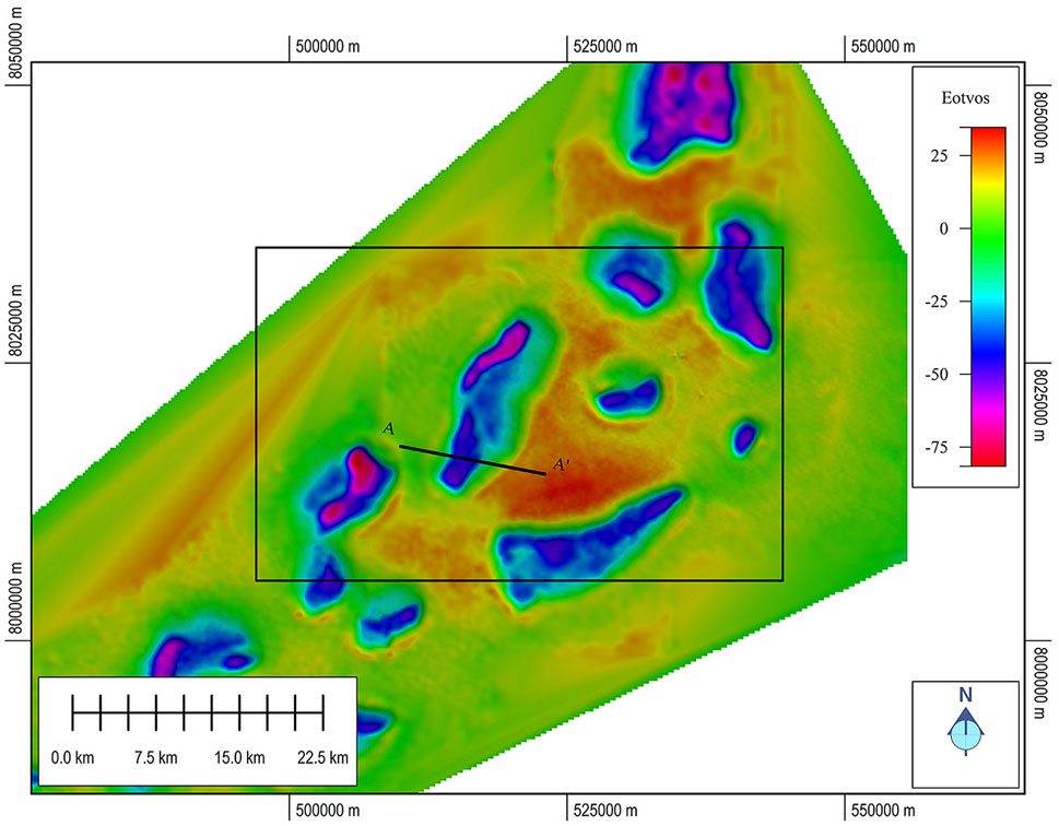
FIGURE 1. G_zz component of gravity gradiometry data used in the inversions. The black square outlines the inversion area. The profile location is shown by the black line.

5.2 Inversion parameters

The 3D voxel-based inversions were all carried out with a parallelized GPU code utilizing a moving sensitivity domain to minimize computation (Cuma et al., 2012; Cuma and Zhdanov, 2014). Voxel size was 200 m laterally with a logarithmic vertical discretization of 40–800 m spaced over 32 layers. Details of the forward modeling methodologies can be found in (Jorgensen and Zhdanov, 2021). All components of the gravity tensor and TMI data were inverted towards density and magnitude of magnetization vector.

The inversions were all terminated when the respective data misfits reached the error level of about 5%. The plot of data misfit versus iteration shown in Figure 2 demonstrates the probabilistic Gramian approach converged to a solution in roughly half the number of iterations as the deterministic Gramian approach. The standalone inversions converged to a solution in less than ten iterations; however, these models exhibited less structural correlation than the models derived from joint inversion.

FIGURE 2

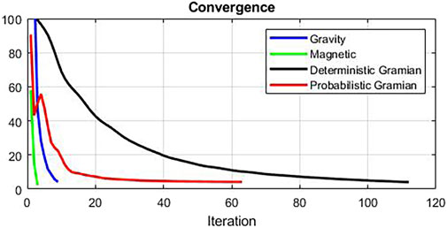
FIGURE 2. Convergence comparison shown as data misfit versus iteration number. The standalone gravity and magnetic inversions are shown by the blue and green lines, respectively. The deterministic and probabilistic Gramian inversions are shown by the black and red lines, respectively.

Figures 3, 4, 5 show the comparison of observed data and data predicted from the different inversion methodologies. The data misfits of approximately 5% are comparable for all inversion methodologies.

FIGURE 3

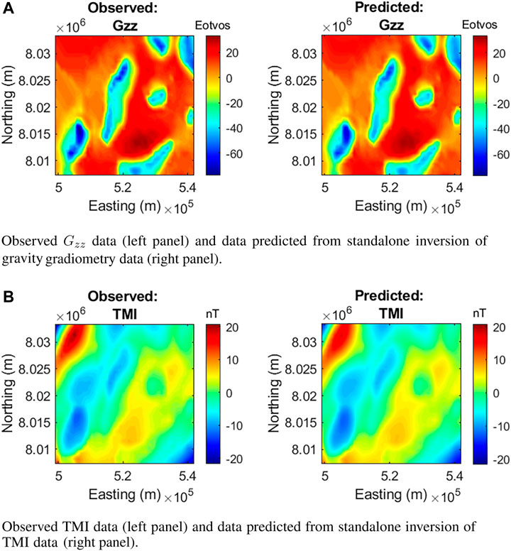
FIGURE 3. Observed and predicted data from standalone inversion. (A) Observed G_zz data (left panel) and data predicted from standalone inversion of gravity gradiometry data (right panel). (B) Observed TMI data (left panel) and data predicted from standalone inversion of TMI data (right panel).

FIGURE 4

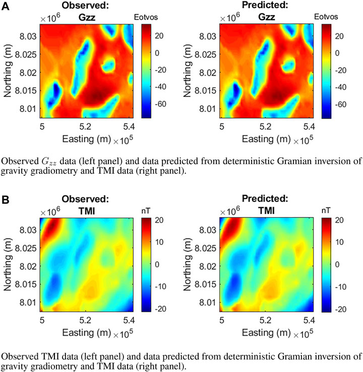
FIGURE 4. Observed and predicted data from deterministic Gramian inversion. (A) Observed G_zz data (left panel) and data predicted from deterministic Gramian inversion of gravity gradiometry and TMI data (right panel). (B) Observed TMI data (left panel) and data predicted from deterministic Gramian inversion of gravity gradiometry and TMI data (right panel).

FIGURE 5

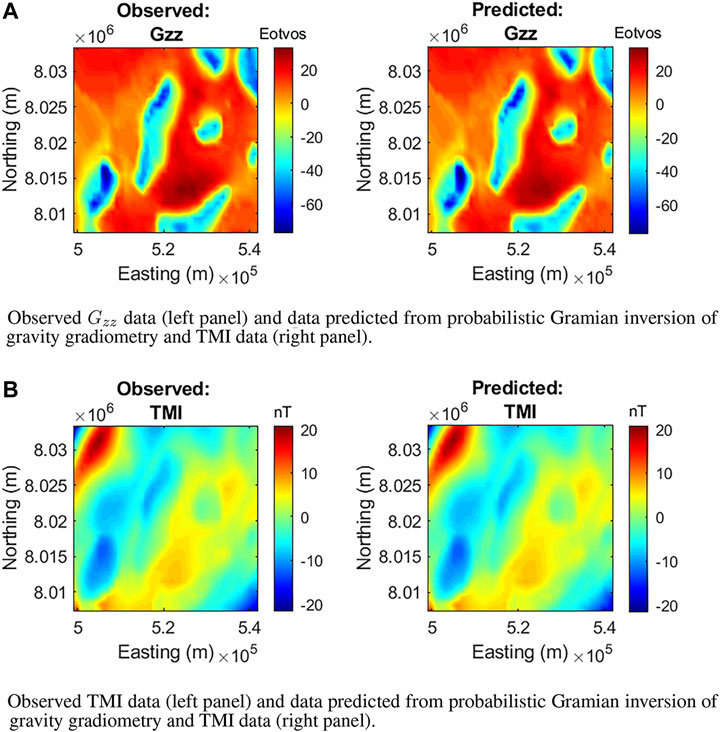
FIGURE 5. Observed and predicted data from probabilistic Gramian inversion. (A) Observed G_zz data (left panel) and data predicted from probabilistic Gramian inversion of gravity gradiometry and TMI data (right panel). (B) Observed TMI data (left panel) and data predicted from probabilistic Gramian inversion of gravity gradiometry and TMI data (right panel).

5.3 Inversion results comparison

5.3.1 Standalone inversion results

Vertical profiles extracted from the 3D voxel models of density and magnetization obtained from standalone inversions of the gravity gradiometry and TMI data, respectively, are shown in Figure 6. A typical density of the base tertiary rocks in the area of investigation is within 2.30–2.38 g/cm³. The Uranus salt diapir is characterized usually by negative density anomalies, which is clearly seen in Figure 6. The negative magnetization within the salt diapir indicates that it is opposite to the direction of the inducing magnetic field, which corresponds to a diamagnetic property of the salt structures. At the same time, the magnetization is positive outside the diapir which is typical for paramagnetic minerals present in Cretaceous sea-bottom layers of the host formations (Paoletti et al., 2020; Tao et al., 2021). Thus, the volume distribution of the density and magnetization, produced by inversion is indicative about the salt diapir structure in the Nordkapp basin. However, while the anomalies in the respective models are roughly coindicent, the gross morphology of the bodies varies widely.

FIGURE 6

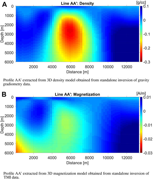
FIGURE 6. Standalone inversion results. (A) Profile AA’ extracted from 3D density model obtained from standalone inversion of gravity gradiometry data. (B) Profile AA’ extracted from 3D magnetization model obtained from standalone inversion of TMI data.

5.3.2 Deterministic Gramian inversion results

The deterministic Gramian inversion improved the structural correlation of the inverse density and magnetization models. Compared to the models obtained from standalone inversions, we see a stronger agreement in gross morphology across the respective models. The vertical profiles extracted from the 3D voxel models of density and magnetization obtained from deterministic Gramian inversion of the gravity gradiometry and TMI data, respectively, are shown in Figure 7).

FIGURE 7

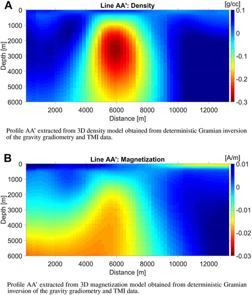
FIGURE 7. Deterministic Gramian inversion results. (A) Profile AA’ extracted from 3D density model obtained from deterministic Gramian inversion of the gravity gradiometry and TMI data. (B) Profile AA’ extracted from 3D magnetization model obtained from deterministic Gramian inversion of the gravity gradiometry and TMI data.

5.3.3 Probabilistic Gramian inversion results

Finally, the same vertical sections extracted from the 3D voxel models of density and magnetization obtained from probabilistic Gramian inversion of the gravity gradiometry and TMI data, respectively, are shown in Figure 8. These models show the strongest degree of correlation across the density and magnetization models, giving a more definitive picture of the Uranus diapir. We can see, indeed, that the structural overhangs necessary for a hydrocarbon trap are absent despite a large salt volume. The poor candidacy for hydrocarbon exploration was confirmed by drilling.

FIGURE 8

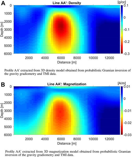
FIGURE 8. Probabilistic Gramian inversion results. (A) Profile AA’ extracted from 3D density model obtained from probabilistic Gramian inversion of the gravity gradiometry and TMI data. (B) Profile AA’ extracted from 3D magnetization model obtained from probabilistic Gramian inversion of the gravity gradiometry and TMI data.

The probabilistic Gramian approach proved to be more numerically stable and efficient, and produced models with enhanced structural correlation.

Petrophysically guided inversion can be a useful tool in refining inversion results (Sun and Li, 2015); however, the a priori petrophysical relations may be unknown. One advantage of the Gramian approach, deterministic or probabilistic, is the oppotunity to see these petrophysical relations in a parametric cross plot of the inverted models. We present cross plots of density versus magnetization for each of the inversion methodologies in Figure 9.

FIGURE 9

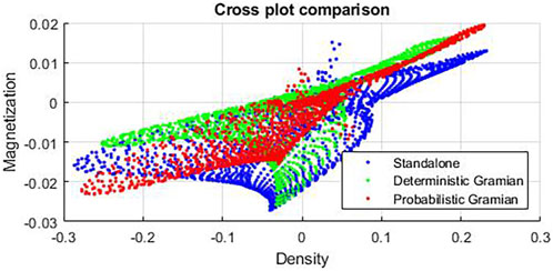
FIGURE 9. Cross plots of the density and magnetization values surrounding the Uranus diapir. The blue dots represent the correlation from the standalone inversions. The green and red dots represent the correlation from the deterministic and probabilistic Gramian inversions, respectively.

The “cloud” of correlations shown by the blue dots in Figure 9 makes it difficult to determine any a priori relations in the standalone inversions. The calculated correlation coefficient for the standalone inversions in the area surrounding the Uranus diapir is 0.7. The cross plots for the deterministic and probabilistic Gramian inversions are shown by the green and red dots in Figure 9, respectively. Compared to the standalone inversions, a clear trend is now discernible in the scattered correlations. The calculated correlation coefficient for the deterministic Gramian is 0.73, which is a marginal improvement over the standalone inversions, and 0.93 for the probabilistic Gramian, which is a significant improvement over the other inversion methodologies.

6 Conclusion

Joint inversion of multiphysics data based on the Gramian constraints represents a powerful tool for integrated interpretation. The Gramian is defined as the determinant of the Gram matrix formed by models of different physical properties of the geologic formations, e.g., density, electrical conductivity, seismic velocity, magnetization, etc. This definition appears naturally in the framework of the deterministic approach to the inverse problem. At the same time, a significant body of research is based on the probabilistic approach to the inversion theory. In this case, the observed data, and the physical models are treated as the realizations of some random variables. The advantage of the probabilistic approach over the deterministic one is that the former provides some valuable statistics about the probability and accuracy of the physical models produced by the inversion.

We have developed and presented joint inversion methods based on the probabilistic approach, which provides insight into the properties of the inversion and helps improve the reliability of the inversion results. This was illustrated in the example from the Nordkapp Basin, where inverted models had a higher structural correlation and the numerical scheme was more efficient compared to the deterministic approach.

We have demonstrated how the joint Gramian-based inversion could be reformulated using the probabilistic approach. The Gramian is an analog of the determinant of the covariance matrix between the different physical properties representing the geologic formations. This helps understand better the role of the Gramian in enforcing the relationships between different physical models. It presents an alternative numerical implementation of the Gramian-type constraints by using the statistical estimates of the components of the covariance matrix.

The incorporation of the covariance in the Gramian constraint is an example of a Gaussian process, and was used to determine the relationship between the model parameters and data with no a priori knowledge. This opens the door to more modern probabilistic approaches, such as empirical Bayes, where model parameters can be estimated directly from the data in areas with little a priori knowledge. Such a prediction will, of course, depend on the amount and veracity of a priori knowledge or training models. Gaussian processes, Bayesian statistics, and empirical Bayes paired with rapidly advancing joint inversion strategies present a promising future for multi-modal geophysical inversion.

Data availability statement

The data analyzed in this study is subject to the following licenses/restrictions: We do not have permission to share the data. Requests to access these datasets should be directed to michael.zhdanov@utah.edu.

Author contributions

MZ was responsible for the theoretical concept. MJ implemented the computer code and conducted the inversions. MZ wrote the first draft of the manuscript. MJ and MT conducted background research on the geologic setting and wrote the example section of the manuscript. All authors contributed to manuscript revision, read, and approved the submitted version.

Acknowledgments

We acknowledge the support of the Consortium for Electromagnetic Modeling and Inversion (CEMI) at the University of Utah, and TechnoImaging. We thank Equinor (formerly Statoil) for providing access to the gravity gradiometry and magnetic data used in the example. The data were gathered by Bell Geospace.

Conflict of interest

MJ was employed by TechnoImaging.

The remaining authors declare that the research was conducted in the absence of any commercial or financial relationships that could be construed as a potential conflict of interest.

Publisher’s note

All claims expressed in this article are solely those of the authors and do not necessarily represent those of their affiliated organizations, or those of the publisher, the editors and the reviewers. Any product that may be evaluated in this article, or claim that may be made by its manufacturer, is not guaranteed or endorsed by the publisher.

Supplementary material

The Supplementary Material for this article can be found online at: https://www.frontiersin.org/articles/10.3389/feart.2023.1127597/full#supplementary-material

References

Afnimar, A., Koketsu, K., and Nakagawa, K. (2002). Joint inversion of refraction and gravity data for the three-dimensional topography of a sediment–basement interface. Geophys. J. Int. 151, 243–254. doi:10.1046/j.1365-246x.2002.01772.x

CrossRef Full Text | Google Scholar

Barth, N. (1999). The gramian and k-volume in n-space: Some classical resultsin linear algebra. J. Young Investigators 2.

Google Scholar

Cuma, M., Wilson, G., and Zhdanov, M. S. (2012). Large-scale 3D inversion of potential field data. Geophys. Prospect. 60, 1186–1199. doi:10.1111/j.1365-2478.2011.01052.x

CrossRef Full Text | Google Scholar

Cuma, M., and Zhdanov, M. S. (2014). Massively parallel regularized 3D inversion of potential fields on CPUs and GPUs. Comput. Geosciences 62, 80–87. doi:10.1016/j.cageo.2013.10.004

CrossRef Full Text | Google Scholar

Dengo, C., and Røssland, K. (1992). Extensional tectonic history of the Western barents sea. In Structural and tectonic modelling and its application to petroleum geology, eds. R. Larsen, H. Brekke, B. Larsen, E. Talleraas, and (Amsterdam: Elsevier), vol. 1 of Norwegian Petroleum Society Special Publications. 91–107. doi:10.1016/B978-0-444-88607-1.50011-5

CrossRef Full Text | Google Scholar

Everitt, W. N. (1958). Some properties of gram matrices and determinants. Q. J. Math. 9, 87–98. doi:10.1093/qmath/9.1.87

CrossRef Full Text | Google Scholar

Fletcher, R. (1995). Practical methods of optimization. John Wiley & Sons.

Google Scholar

Foster, M. (1961). An application of the Wiener-Kolmogorov smoothing theory to matrix inversion. J. Soc. Industrial Appl. Math. 9, 387–392. doi:10.1137/0109031

CrossRef Full Text | Google Scholar

Franklin, J. N. (1970). Well-posed stochastic extensions of ill-posed linear problems. J. Math. Analysis Appl. 31, 682–716. doi:10.1016/0022-247x(70)90017-x

CrossRef Full Text | Google Scholar

Gallardo, L. A., and Meju, M. A. (2003). Characterization of heterogeneous near-surface materials by joint 2D inversion of DC resistivity and seismic data. Geophys. Res. Lett. 30, 1658. doi:10.1029/2003gl017370

CrossRef Full Text | Google Scholar

Gallardo, L. A., and Meju, M. A. (2007). Joint two-dimensional cross-gradient imaging of magnetotelluric and seismic traveltime data for structural and lithological classification. Geophys. J. Int. 169, 1261–1272. doi:10.1111/j.1365-246x.2007.03366.x

CrossRef Full Text | Google Scholar

Gallardo, L. A., and Meju, M. A. (2004). Joint two-dimensional dc resistivity and seismic travel-time inversion with cross-gradients constraints. J. Geophys. Res. 109, B03311. doi:10.1029/2003jb002716

CrossRef Full Text | Google Scholar

Gallardo, L. A., and Meju, M. A. (2011). Structure-coupled multi-physics imaging in geophysical sciences. Rev. Geophys. 49, RG1003. doi:10.1029/2010rg000330

CrossRef Full Text | Google Scholar

Gallardo, L. A. (2007). Multiple cross-gradient joint inversion for geospectral imaging. Geophys. Res. Lett. 34, L19301. doi:10.1029/2007gl030409

CrossRef Full Text | Google Scholar

Gao, G., Abubakar, A., and Habashy, T. M. (2012). Joint petrophysical inversion of electromagnetic and full-waveform seismic data. Geophysics 77, WA3–WA18. doi:10.1190/geo2011-0157.1

CrossRef Full Text | Google Scholar

Gernigon, L., Brönner, M., Fichler, C., Løvås, L., Marello, L., and Olesen, O. (2011). Magnetic expression of salt diapir–related structures in the Nordkapp Basin, Western Barents Sea. Geology 39, 135–138. doi:10.1130/G31431.1

CrossRef Full Text | Google Scholar

Giraud, J., Ogarko, V., Lindsay, M., Pakyuz-Charrier, E., Jessell, M., and Martin, R. (2019). Sensitivity of constrained joint inversions to geological and petrophysical input data uncertainties with posterior geological analysis. Geophys. J. Int. 218, 666–688. doi:10.1093/gji/ggz152

CrossRef Full Text | Google Scholar

Giraud, J., Pakyuz-Charrier, E., Jessell, M., Lindsay, M., Martin, R., and Ogarko, V. (2017). Uncertainty reduction through geologically conditioned petrophysical constraints in joint inversion. Geophysics 82, ID19–ID34. doi:10.1190/geo2016-0615.1

CrossRef Full Text | Google Scholar

Hokstad, K., Fotland, B., Mackenzie, G., Antonsdottir, V., Foss, S., Stadtler, C., et al. (2011). Jt. imaging Geophys. data Case Hist. Nordkapp Basin, Barents Sea, 1098–1102. doi:10.1190/1.3627395

CrossRef Full Text

Hoversten, G. M., Cassassuce, F., Gaskeripova, E., Newman, G. A., Chen, J., Rubin, Y., et al. (2006). Direct reservoir parameter estimationusing joint inversion of marine seismic AVA and CSEM data. Geophysics 71, C1–C13. doi:10.1190/1.2194510

CrossRef Full Text | Google Scholar

Jackson, D. D. (1972). Interpretation of inaccurate, insufficient and inconsistent data. Geophys. J. R. Astronomical Soc. 28, 97–109. doi:10.1111/j.1365-246x.1972.tb06115.x

CrossRef Full Text | Google Scholar

Jorgensen, M., and Zhdanov, M. S. (2021). Recovering magnetization of rock formations by jointly inverting airborne gravity gradiometry and total magnetic intensity data. Minerals 11, 366. doi:10.3390/min11040366

CrossRef Full Text | Google Scholar

Moorkamp, M., Heincke, B., Jegen, M., Robert, A. W., and Hobbs, R. W. (2011). A framework for 3-D joint inversion of MT, gravity and seismic refraction data. Geophys. J. Int. 184, 477–493. doi:10.1111/j.1365-246x.2010.04856.x

CrossRef Full Text | Google Scholar

Moorkamp, M., Lelievre, P., Linde, N., and Khan, A. (2016). Integrated imaging of the earth: Theory and applications. Geophysical Monograph Series (Wiley).

Google Scholar

Paoletti, V., Milano, M., Baniamerian, J., and Fedi, M. (2020). Magnetic field imaging of salt structures at nordkapp basin, barents sea. Geophys. Res. Lett. 47, e2020GL089026. doi:10.1029/2020gl089026

CrossRef Full Text | Google Scholar

Ross, S. (2010). A First Course in Probability 2010. 8th edition. Upper Saddle River, NJ: Prentice Hall

Google Scholar

Stadtler, C., Fichler, C., Hokstad, K., Myrlund, E. A., Wienecke, S., and Fotland, B. (2014). Improved salt imaging in a basin context by high resolution potential field data: Nordkapp basin, barents sea. Geophys. Prospect. 62, 615–630. doi:10.1111/1365-2478.12101

CrossRef Full Text | Google Scholar

Sun, J., and Li, Y. (2015). Multidomain petrophysically constrained inversion and geology differentiation using guided fuzzy c-means clustering. Geophysics 80, ID1–ID18. doi:10.1190/geo2014-0049.1

CrossRef Full Text | Google Scholar

Tao, M., Jorgensen, M., and Zhdanov, M. S. (2021). Mapping the salt structures from magnetic and gravity gradiometry data in Nordkapp Basin. Barents Sea, 874–878. doi:10.1190/segam2021-3583664.1

CrossRef Full Text | Google Scholar

Tarantola, A. (1987). Inverse problem theory. Elsevier.

Google Scholar

Tarantola, A. (2005). Inverse problem theory and methods for model parameter estimation. Philadelphia, PA: SIAM.

Google Scholar

Tarantola, A., and Valette, B. (1982). Generalized nonlinear inverse problems solved using the least squares criterion. Rev. Geophys. Space Phys. 20, 219–232. doi:10.1029/rg020i002p00219

CrossRef Full Text | Google Scholar

Tu, X., and Zhdanov, M. S. (2022). Joint focusing inversion of marine controlled-source electromagnetic and full tensor gravity gradiometry data. Geophysics 87, K35–K47. doi:10.1190/geo2021-0691.1

CrossRef Full Text | Google Scholar

Tu, X., and Zhdanov, M. S. (2021). Joint focusing inversion of marine controlled-source electromagnetic and full tensor gravity gradiometry data: Case study of the Nordkapp Basin in Barents Sea. Norway, 1746–1750. doi:10.1190/segam2021-3581155.1

CrossRef Full Text | Google Scholar

Zhdanov, M. S. (2002). Geophysical inverse theory and regularization problems. Elsevier.

Google Scholar

Zhdanov, M. S. (2015). Inverse theory and applications in geophysics. Elsevier.

Google Scholar

Zhdanov, M. S., Gribenko, A. V., Wilson, G., and Funk, C. (2012b). 3D joint inversion of geophysical data with gramian constraints: A case study from the carrapateena iocg deposit, south Australia. Lead. Edge 31, 1382–1388. doi:10.1190/tle31111382.1

CrossRef Full Text | Google Scholar

Zhdanov, M. S., Gribenko, A. V., and Wilson, G. (2012a). Generalized joint inversion of multimodal geophysical data using Gramian constraints. Geophys. Res. Lett. 39, L09301. doi:10.1029/2012gl051233

CrossRef Full Text | Google Scholar

Zhdanov, M. S., Jorgensen, M., and Cox, L. (2021). Advanced methods of joint inversion of multiphysics data for mineral exploration. Geosciences 11, 262. doi:10.3390/geosciences11060262

CrossRef Full Text | Google Scholar