Surface impacts and associated mechanisms of a moisture intrusion into the Arctic observed in mid-April 2020 during MOSAiC

1 Introduction

The Arctic has warmed nearly four times faster than the globe (Rantanen et al., 2022), a phenomenon termed Arctic amplification. The main underlying mechanisms have been reviewed recently (Previdi et al., 2021; Taylor et al., 2022; Wendisch et al., 2022). The poleward atmospheric transport of dry-static and latent energy plays a critical role for the seasonality and magnitude of Arctic air temperatures, and long-term changes in this transport are likely one of the driving forces of Arctic amplification (e.g., Graversen and Burtu, 2016; Mewes and Jacobi, 2019; Naakka et al., 2019). These poleward energy transports are tightly coupled to local feedback mechanisms. Of particular importance are those related to cloud formation/dissipation, thermodynamic phase partitioning, and liquid-water-to-ice phase transitions within atmospheric boundary layer clouds during air mass transformation processes (Pithan et al., 2018).

Besides long-term transport and its changes, episodic variability is also crucial. Such variability is particularly caused by distinct events of warm and moist air intrusions (WAIs) from the mid-latitudes into the Arctic. In fact, 60%–90% of poleward moisture transport occurs during only 10% of the time (Johansson et al., 2017; Nash et al., 2018; Pithan et al., 2018). WAIs take place throughout the year, move along season-dependent pathways, and are associated with specific large-scale atmospheric circulation patterns and individual weather events (Henderson et al., 2021), such as synoptic cyclones and the occurrence of atmospheric blocking (e.g., Binder et al., 2017; Fearon et al., 2021; Murto et al., 2022; Papritz et al., 2022).

The related heat and moisture transport into the Arctic contributes to the so-called water vapor triple effect, i.e., warming caused by condensation, the greenhouse effect of water vapor, and the mostly warming effect due to clouds, in particular during polar night (Taylor et al., 2022). This directly and indirectly impacts the surface energy budget (SEB) by cloud-radiation feedbacks (e.g., Wendisch et al., 2019; You et al., 2021; 2022; Bresson et al., 2022). Cloud radiative forcing especially of liquid-water containing clouds (Shupe et al., 2022) causes surface warming (e.g., Woods and Caballero, 2016; Dahlke and Maturilli, 2017; Graham et al., 2017; Messori et al., 2018) and can trigger sea-ice melt in spring-summer or retarded sea-ice growth in winter seasons (e.g., Park et al., 2015; Tjernström et al., 2015; Boisvert et al., 2016; Mortin et al., 2016; Persson et al., 2016; Li et al., 2022; Liang et al., 2022). WAIs also cause precipitation in different phases (rain and/or snow) in the Arctic (e.g., Viceto et al., 2022). This topic has rarely been studied, even though precipitation further influences the sea ice, for example, by modifying the thermal insulation or surface albedo (Webster et al., 2018).

Because of the important role of WAIs for the Arctic climate in general, and for Arctic amplification in particular, a better quantification of the impacts of WAIs on the SEB and precipitation is required. For this purpose, moisture sources, pathways into the Arctic and related large-scale flow need to be investigated; the air mass transformations along the flow and involved processes have to be better understood (Pithan et al., 2018; Henderson et al., 2021; Wendisch et al., 2021; Taylor et al., 2022).

To pursue the aims discussed above, we follow the approach of combining both i) observations and process modeling, as well as ii) Eulerian and Lagrangian approaches. In this study, we apply this strategy to a case study of a WAI observed during the Multidisciplinary drifting Observatory for the Study of Arctic Climate (MOSAiC) expedition, which provides unique observations from aboard the research vessel (RV) Polarstern as well as from the surrounding of it in the central Arctic (Nicolaus et al., 2022; Rabe et al., 2022; Shupe et al., 2022). The selected WAI occurred in mid-April 2020. This event is particularly interesting because of three aspects: i) It consisted of two separate intrusions within about a week, connected to different synoptic circulation patterns (Magnusson et al., 2020), ii) It was a record-breaking event, i.e., extreme with regard to moisture, air temperature, and longwave downward radiation at the surface, all being the highest for this location and time of year in the past 40 years (Rinke et al., 2021), and iii) It carried air pollutants from northern Eurasia and caused drastic changes in the atmospheric composition, aerosol characteristics, and cloud condensation nuclei concentrations in the central Arctic (Dada et al., 2022). This study aims to explore in detail this WAI event with respect to the following three specific objectives: (O1) Quantify the synoptic situation and transport, (O2) Understand air mass transformation via cloud processes, and (O3) Investigate related surface impacts in terms of the SEB and precipitation.

2 Complementary analysis methods

We apply a number of different research tools to thoroughly analyze this WAI event in unprecedented detail. These tools provide highly complementary perspectives, including a detailed examination of ERA5 reanalysis data to provide a large-scale context, trajectory calculations to track air mass evolution, Lagrangian Large-Eddy Simulations (LES) to demonstrate the involved atmosphere-cloud processes in detail, regional limited-area modeling (LAM) to explore the sensitivity of the intrusion to moisture parameters, and finally MOSAiC and novel satellite observations to verify model results and offer insight into atmosphere-surface interactions.

2.1 Observations

We use the MOSAiC measurements listed in Table 1 for the evaluation of the simulations. For details of the observational data, we refer to the references given in the table. Near-surface temperature, relative humidity, air pressure, and atmospheric SEB observations (consisting of radiative, turbulent sensible and latent heat fluxes) are obtained from the Met Tower and two autonomous Atmospheric Surface Flux Stations (Shupe et al., 2022). Data from the Humidity and Temperature Profiler (HATPRO) is used (Walbröl et al., 2022), from which Integrated Water Vapor (IWV) and Liquid Water Path (LWP) data are derived. Remote sensing measurements from cloud radar, lidar and microwave radiometer at RV Polarstern are combined via the Cloudnet algorithm to investigate the vertical distribution of cloud liquid and ice water content (LWC and IWC) (Illingworth et al., 2007). The ice water path (IWP) is calculated by vertical integration of the IWC profiles. As Cloudnet does not differentiate between suspended and falling solid hydrometeors, it actually outputs the combined ice and snow water path (IWP + SWP).

TABLE 1

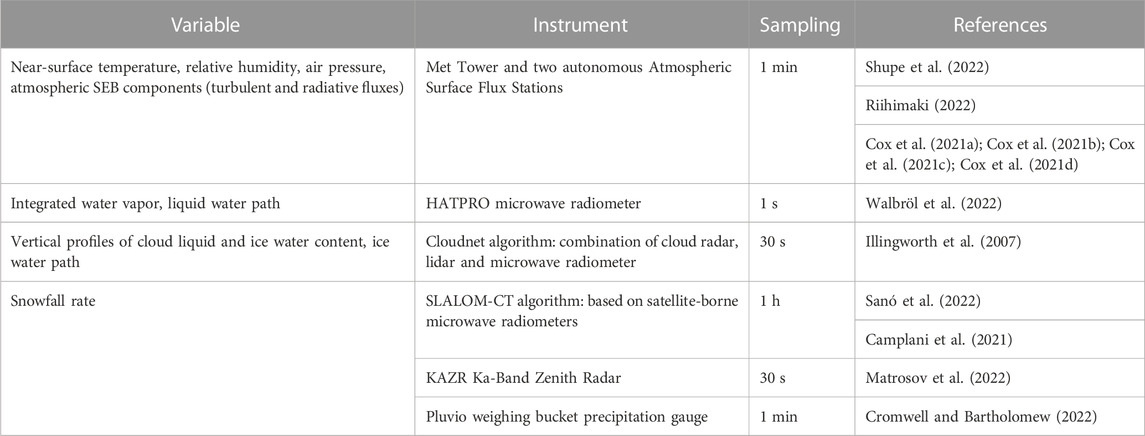
TABLE 1. Overview of MOSAiC measurements used in this study. For all analyses, the original data was averaged to hourly means.

Due to the high uncertainty of snowfall measurements, we base our analysis on ERA5 reanalysis data and on three additional observational sources. i) Satellite data: The surface snowfall rate estimates are obtained from the Advanced Technology Microwave Sounder observations (ATMS) by using the Snow retrievaL ALgorithm fOr gpM–Cross Track (SLALOM-CT) (Sanó et al., 2022). The ATMS instrument provides global coverage and a relatively short revisit time at high latitudes of about one hour. The high frequency channels are the most sensitive to the presence of snow in the atmosphere (Weng et al., 2012). ATMS observations from the near-polar orbiting satellites Suomi National Polar-orbiting Partnership (SNPP) and NOAA-20 are used in this work. ii) Ka-Band Zenith Radar (KAZR): The snowfall rate has been calculated at the MOSAiC site using the radar reflectivity (Matrosov et al., 2022). iii) Pluvio: This is a weighing bucket precipitation gauge (Cromwell and Bartholomew, 2022). During MOSAiC, Pluvio was installed at the ice camp and sheltered by a double windshield to reduce the influences of blowing snow.

2.2 Reanalysis data

We use the European Centre for Medium-range Weather Forecast’s (ECMWF) fifth generation reanalysis data set ERA5 (Hersbach et al., 2020), which is appropriate here because of its high resolution, both horizontally (ca. 30 km) and temporally (1-hourly), and the advanced 4D-var assimilation scheme. Compared to observations and other reanalyses, ERA5 offers an improved performance over the Arctic (Graham et al., 2019a; b). The ERA5 data is used to characterize the integrated water vapor transport (IVT), IWV, air temperature at 2 m height (T_2m), equivalent potential temperature at 850 hPa (θ_e 850 hPa), mean sea level pressure (SLP), precipitation, snowfall, cloud properties, and SEB components.

2.3 Lagrangian trajectories

Lagrangian trajectories are calculated using LAGRANTO (Sprenger and Wernli, 2015). The required wind fields are retrieved from ERA5 reanalysis on 137 model levels and its native spatiotemporal resolution. ERA5 wind fields have been used in many recent studies relying on trajectory analysis in the Arctic (e.g., Ali and Pithan, 2020; You et al., 2021; 2022; Papritz et al., 2022). Notably, during the WAI period in mid-April 2020, 4 radiosondes were launched daily at different locations upstream of RV Polarstern, and additional 7 radiosondes daily directly from RV Polarstern. All of those were assimilated by ECMWF, which greatly helped to improve the Arctic forecast (ECMWF, 2020) as well as reliability of trajectory calculations.

To study the origin of the air masses that arrive at RV Polarstern, an extensive ensemble of trajectories is computed. The trajectories are initiated throughout the vertical column above the hourly position of RV Polarstern and calculated 5 days backward. Vertically, they are spaced from 0.1 km to 12 km above ground in 0.5 km steps. Horizontally, trajectory starting points are evenly spaced every 3 km in a circle of 20 km radius around RV Polarstern. For further analysis, statistics of ERA5-derived meteorological parameters during the previous 5 days along the trajectories are extracted. In a first step, the following statistics are calculated for each individual trajectory:

• lat_med (°N) Median latitude the air masses resided at.

• z_min (km) Minimum altitude the air masses resided at.

• Δθ K) Maximum change in potential temperature. This is calculated with respect to the final state above RV Polarstern. Δθ is positive (negative) if diabatic heating (cooling) dominated.

• Δq (g kg^-1) Maximum change in specific humidity. Δq is positive (negative) if moistening (loss of moisture) is the dominating mechanism along air mass drift towards RV Polarstern.

• WVT_max (g kg^-1 m s^-1) Maximum water vapor transport. This is calculated as the product of specific humidity and scalar wind speed, and is not to be confused with IVT (which is vertically integrated WVT).

• ∂T/∂t_lhr,max (K d^-1) Maximum temperature tendency due to latent heat release during cloud formation. This is extracted from ERA5 model physics similarly as described by You et al. (2021).

In order to depict mean air mass properties, for each ensemble set started at an individual time and location, these statistics are then averaged (mean value).

We calculate further trajectories to investigate the large-scale flow. For this, the air parcels are started in a box evenly spaced every 30 km along latitude/longitude, spanning 5°W to 30°E and 81–87°N (i.e., centered around RV Polarstern; see Supplementary Figure S1). Calculations are started on 19 April 2020, 12 UTC, and extended 24 h backward and 30 h forward in time. Vertically, air parcels are started at pressure levels between 700 hPa and 950 hPa in 10 hPa steps. Similar to others (e.g., You et al., 2021), we extract ensemble averages of meteorological parameters along the trajectories.

2.4 Atmospheric river detection

To estimate the precipitation caused by the WAIs, the spatial shape of the WAIs is approximated by applying the atmospheric river detection algorithm of Guan et al. (2018) and using ERA5 reanalysis data. In this algorithm, the shape of the atmospheric river component of the WAI is constrained by the following characteristics: i) For each grid point, IVT must at least exceed the local 85th percentile from climatology, ii) The overall length must be a minimum of 2,000 km, and iii) The length/width ratio must be greater than 2. If an IVT object obtained via the 85th percentile threshold fails to fulfill geometric requirements, IVT thresholds are incrementally increased. A maximum 95th percentile threshold is used.

2.5 Large-scale energy transport and circulation regimes

The vertically integrated atmospheric horizontal energy transport (IET) is calculated and split into latent and dry static components following Graversen and Burtu (2016):

$\mathit{I}\mathit{E}\mathit{T}=\underset{\mathbf{m}\mathbf{o}\mathbf{i}\mathbf{s}\mathbf{t}\mathbf{s}\mathbf{t}\mathbf{a}\mathbf{t}\mathbf{i}\mathbf{c}}{\underbrace{\stackrel{\mathbf{l}\mathbf{a}\mathbf{t}\mathbf{e}\mathbf{n}\mathbf{t}}{\overbrace{{\displaystyle \underset{{\mathit{p}}_{\mathbf{s}}}{\overset{\mathbf{0}}{\int }}}\overrightarrow{\mathit{v}}\mathit{q}{\mathbf{L}}_{\mathbf{v}}\frac{\mathbf{d}\mathit{p}}{\mathbf{g}}}}+\stackrel{\mathbf{d}\mathbf{r}\mathbf{y}\mathbf{s}\mathbf{t}\mathbf{a}\mathbf{t}\mathbf{i}\mathbf{c}}{\overbrace{{\displaystyle \underset{{\mathit{p}}_{\mathbf{s}}}{\overset{\mathbf{0}}{\int }}}\overrightarrow{\mathit{v}}\left({\mathbf{c}}_{\mathbf{p}}\mathit{T}+\mathbf{g}\mathit{z}\right)\frac{\mathbf{d}\mathit{p}}{\mathbf{g}}}}}}+{\displaystyle \underset{{\mathit{p}}_{\mathbf{s}}}{\overset{\mathbf{0}}{\int }}}\overrightarrow{\mathit{v}}\frac{\mathbf{1}}{\mathbf{2}}{\left(\overrightarrow{\mathit{v}}\right)}^{\mathbf{2}}\frac{\mathbf{d}\mathit{p}}{\mathbf{g}}$

where p is pressure (hPa), p_s surface pressure (hPa), $\overrightarrow{\mathit{v}}$ = (u,v) horizontal wind vector with components u and v (m s^-1), L_v = 2,260 kJ kg^-1 the latent heat of vaporization, q specific humidity (kg kg^-1), c_p = 1.005 kJ kg^-1 K⁻¹ specific heat capacity at constant pressure, T temperature (K), g = 9.81 m s^-2 gravitational acceleration, and z height (m).

Horizontal energy transport is calculated from 6-hourly data of ERA5 reanalysis on model levels before vertical integration and daily averaging is performed. As suggested by Trenberth (1991) and used in several recent publications (e.g., Lembo et al., 2019; Liu et al., 2020), a barotropic wind-field correction is applied to the wind before the calculations of the energy transport is done to account for spurious mass-fluxes due to the assimilation procedure of reanalyses. Climatological values are calculated from all April days of the years 1979–2020. The net energy transport across the Arctic Circle is derived from the meridional component of the vertically integrated energy transport and integration along 66.3°N.

To identify preferred states of the large-scale atmospheric circulation, the regime analysis described in Crasemann et al. (2017) is applied to daily ERA5 SLP anomalies of spring (March to June) 1979–2020 over the North-Atlantic/European region. In order to determine five atmospheric circulation regimes, a k-means clustering algorithm is carried out in a reduced phase space spanned by the five leading empirical orthogonal functions (Hannachi et al., 2017; Falkena et al., 2020).

2.6 High-resolution process modeling

2.6.1 Large-Eddy simulations (LES)

The transformation of an Arctic air mass is studied using targeted LES experiments at turbulence- and cloud-resolving resolutions similar to Bretherton et al. (1999, 2010). In this method, the upper-level profile above the boundary layer and the surface boundary condition remain tightly constrained by reanalysis or observational data. In contrast, the resolved turbulence and associated mixed-phase clouds inside the LES domain are free to develop, and can respond to the changing meteorological conditions along the trajectory. In this setting the transformation can be investigated at process level, for example, through targeted sensitivity experiments on conditions of interest.

Lagrangian LES are performed with the DALES code (Heus et al., 2010) and forced by ERA5 data, following the method introduced by Van Laar et al. (2019) and Neggers et al. (2019). Nudging is applied above the thermal inversion, which marks the boundary layer top. Nudging linearly increases in intensity across a 1 km deep transition layer towards full nudging above, at a relaxation timescale of 30 min. Below the inversion, no nudging is applied, leaving the turbulence and clouds free to develop. For radiation, a multi-waveband transfer model is used in combination with a Monte Carlo approach (Pincus and Stevens, 2009). The microphysics follow a two-moment scheme with the five hydrometeor types of Seifert and Beheng (2006), albeit with the following modification: The Cloud Condensation Nuclei (CCN) concentration (N_CCN) is prognostic, meaning it can evolve from its initial value as a result of processes such as advection, diffusion, and microphysical transformations. Simulations with three different N_CCN are conducted, with the following rationale: i) N_CCN = 10 cm^-3 represents very clean conditions, ii) N_CCN = 100 cm^-3 is typical for the wintertime Arctic, and iii) N_CCN = 1,000 cm^-3 is a highly polluted state; latter order of magnitude has recently been reported for the first half of the WAI event observed in mid-April 2020 (Dada et al., 2022). The simulations are initialized upstream of RV Polarstern at 0 UTC on 19 April. The LES domain is a cube with a length of 12.8 km in all three directions. The resolution of the simulation is 50 m in both horizontal directions. To prevent reflection of gravity waves from the domain top, a sponge layer is applied in the top 25% of the domain. The vertical resolution is telescopic, starting with 20 m at the bottom of the boundary layer and extending with altitude to 140 m at the top of the domain.

2.6.2 Limited area modeling (ICON-LAM)

To study the moisture intrusion event on a large scale with high resolution, we use the German weather and climate model ICON (Icosahedral Non-hydrostatic Model; Zängl et al., 2014) in the limited area mode (ICON-LAM). Simulations are performed over a circum-Arctic domain (covering 65–90°N) at a 6 km horizontal resolution (R03B08 in ICON terminology). The simulations are initialized from global ICON analysis at 13.15 km resolution (R03B07), which also serves as the 3-hourly lateral and lower boundary forcing. Our setup uses the single-moment microphysics scheme (Doms et al., 2011), which predicts the specific mass content of five hydrometeor categories (cloud liquid water, rain water, cloud ice, snow, graupel), and is recommended for LAM simulations (Prill et al., 2020). For radiation, the ecRad from ECMWF (Hogan and Bozzo, 2018) and for shallow convection the Tiedtke–Bechtold convection scheme (Tiedtke, 1989; Bechtold et al., 2008) are applied. A bulk-thermodynamic sea-ice model (Mironov et al., 2012) is applied with an adjusted heat capacity as introduced by Littmann (2022). For more details on the ICON model and its LAM setup we refer to Prill et al. (2020) and Bresson et al. (2022).

ICON-LAM is used to explore the sensitivity of the WAI with respect to the moisture inflow. In a sensitivity run, the amount of moisture at the lateral boundaries is reduced by a maximum of 30% (Supplementary Figure S1). To ensure that the reduction is only applied at the longitudes where the WAI penetrates into the Arctic, the specific humidity at the boundaries is multiplied by a Gaussian distribution centered at 330°E with a standard deviation of 15°. The reduction by a maximum of 30% is chosen as the event was characterized by about 30% higher IWV than climatology during this time and region, based on ERA5. The ICON-LAM simulations are initialized on 17 April at 18 UTC and run until 21 April, 0 UTC. We analyze hourly output at a latitude-longitude-grid with 0.054° spacing.

3 Results and discussion

We bring the broad range of observational and modeling tools together to describe key aspects of the mid-April 2020 WAI. The analysis first addresses the large-scale setting of the event (Section 3.1). Next, it focuses on the characteristics of the WAI as it passed over RV Polarstern, using the unique MOSAiC observations (Section 3.2). Expanding the Eulerian viewpoint with Lagrangian trajectory analysis, the evolution of the air masses along their drift into the Arctic is discussed (Section 3.3). We examine how the air masses observed at RV Polarstern relate to their origin, and how variations in the initial conditions, such as CCN concentration or lateral moisture influx, may impact the atmospheric state as observed at the shipborne site, and further downstream in the central Arctic. Finally, the impacts of this WAI on the surface are quantified (Section 3.4).

3.1 Large-scale setting of the event

3.1.1 Synoptic overview and circulation regimes

The WAI event consists of two distinct, consecutive intrusions characterized by record-breaking anomalies in T_2m as well as in IWV (Rinke et al., 2021; Section 3.2). In terms of preferred atmospheric circulation regimes (Figure 1A), the initiation of these intense transport events is characterized by a transition from an Icelandic high - Siberian low dipole to a positive North Atlantic Oscillation pattern persisting between 13–19 April.

FIGURE 1

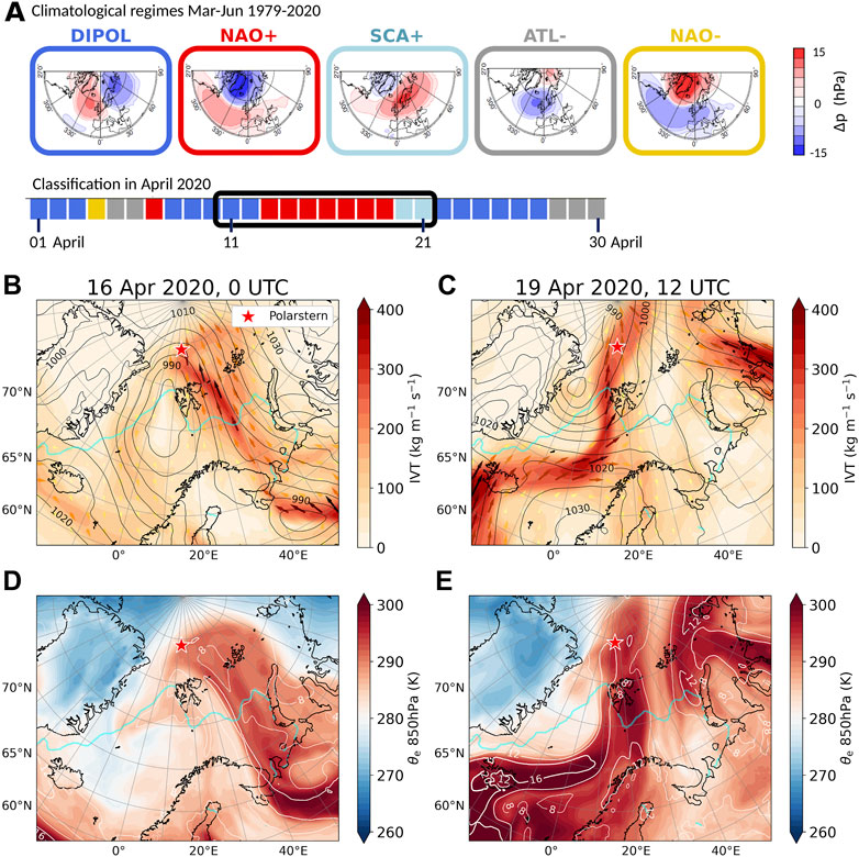
FIGURE 1. (A) Spring circulation regimes in ERA5 reanalysis. Upper panel: five preferred circulation regime patterns during spring time (MAMJ) identified as dipole (DIPOL), positive and negative North Atlantic Oscillation (NAO+, NAO-), Scandinavian blocking (SCA+) and Atlantic low (ATL-). Lower panel: classification during April 2020, with 11–21 April 2020 marked by a black frame. (B–E) Synoptic overview based on ERA5 centered on 16 April 2020, 0 UTC and 19 April 2020, 12 UTC. (B,C) IVT (color shading and arrows), sea level pressure (black isobars; hPa); (D,E) 850 hPa equivalent potential temperature θ_e (color shading), IWV (white isolines; kg m^-2). In each graph the red star shows the locations of RV Polarstern and the cyan line indicates the sea-ice margin based on 15% sea-ice concentration from ERA5.

For the first intrusion, which peaks at the MOSAiC site on 16 April, a corridor of increased IVT and IWV (Figures 1B, D) originating in northwestern Russia and passing the Barents Sea is found (Supplementary Figure S2). In the Barents Sea region, the event is associated with T_2m anomalies exceeding climatological mean values (1979–2020, ERA5) by 8 K. Synoptically, a low-pressure system just west of Svalbard and a high-pressure system to the northeast of Novaya Zemlya facilitate this transport. The resulting pressure dipole pushes warm and moist air northwards. Observations of high aerosol particle concentrations at the MOSAiC site support an origin in the vicinity of industrial activities in northwestern Russia (Dada et al., 2022).

Three days later, on 19 April and during the second intrusion peak recorded by MOSAiC (Figures 1C, E), the low pressure system shifts towards the northeast of Greenland while two high pressure systems evolve, centered around Novaya Zemlya and Norway. Accordingly, the 20–21 April circulation is classified as Scandinavian blocking (Figure 1A), which favors warm and moist air transport across the Fram Strait. This agrees with previous findings that episodes of WAIs to the Arctic are often related to Scandinavian/Ural blocking (Henderson et al., 2021). As a result, a corridor of IVT above 300 kg m⁻¹ s⁻¹ forms from the North Atlantic over Iceland towards the central Arctic. Our trajectory analyses show that the corridor during 2020 is initially positioned over Greenland, and only later shifts to the Fram Strait/Iceland region (Section 3.2). In springtime, the North Atlantic WAI corridor is climatologically favored and has been reported to yield the most intense events (e.g., Mewes and Jacobi, 2019; Nygård et al., 2020; Papritz et al., 2022).

3.1.2 Meridional energy transport

The WAI is characterized by an increased horizontal transport of moist static energy (Figure 2A). The transport anomalies occur along two pathways: While the first intrusion (16 April) shows a connection to the West-Siberian lowlands, the second one (19 April) is linked with an enhanced energy transport from the North Atlantic. This agrees with the already discussed large-scale flow. In this section, we focus on the latent energy transport, which strongly influences water vapor content and cloud formation. Compared to the April climatology, where the meridional latent energy transport has maxima over the Pacific and western North Atlantic/Eastern North America and is rather weak at higher latitudes, the two episodes in April 2020 stand out as intense poleward energy transport events.

FIGURE 2

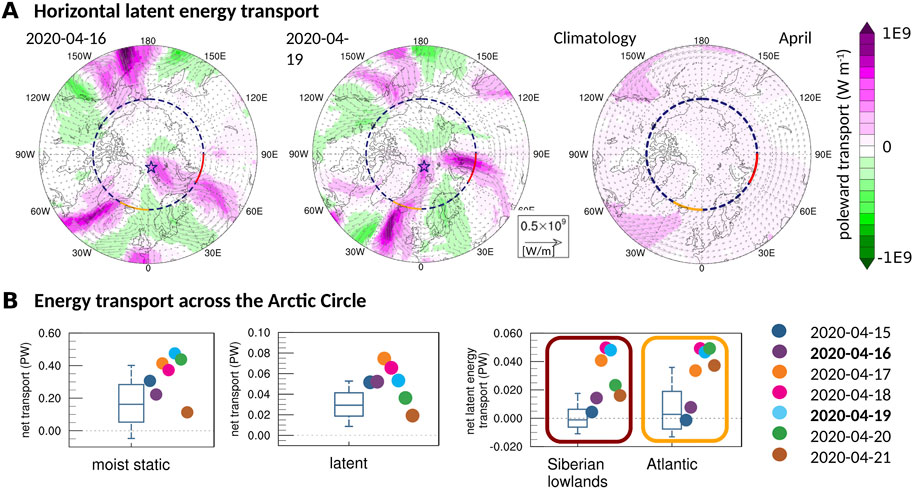
FIGURE 2. (A) Vertically integrated horizontal latent energy transport (arrows), poleward component (pink) and equatorward component (green) on 16 April (left), 19 April (middle), and April climatology from 1979–2020 (right), based on ERA5 reanalysis. The Arctic Circle is marked with a stippled line, the Atlantic segment in orange, the Siberian lowlands segment in red, the position of RV Polarstern with a star. (B) Daily mean net transport across the Arctic Circle in April; moist static energy (left), latent energy (middle), latent energy of Atlantic and Siberian lowlands segments (right). Box plots show the climatology of days in April 1979–2020 from ERA5 reanalysis. Whiskers show the lower decile, lower quartile, median, upper quartile, and upper decile. Colored dots indicate the days of April 2020, from 15 to 21 April.

The analysis of the daily net meridional transport of moist static energy and its latent energy component across the Arctic Circle shows that all days within 15–20 April exhibit strong poleward transport of energy (Figure 2B). The total moist static energy transport into the Arctic exceeds the 90th percentile of the April climatology for April 17, 19 and 20. While the moist static transport is dominated by the dry static component, the latent energy component shows the strongest anomalies. Here, all days between 15–19 April exceed the 90th percentile of the April climatology.

Splitting this further up into the Siberian lowland and Atlantic sections, even stronger anomalies emerge. The first intrusion episode with the pathway from West Siberia is exceptional, with the latent energy transport on 17 April above the 95th percentile of the climatology in that area. Indeed, studies have shown that this Siberian pathway is gaining importance in recent decades (Komatsu et al., 2018; Mewes and Jacobi, 2019). To explain this, several studies have linked the marked retreat of sea ice in the Barents Sea to enhanced local evaporation, moistening, and cyclone-associated precipitation (e.g., Rinke et al., 2019; Crawford et al., 2022), while Pithan and Jung (2021) have questioned the role of local sea-ice changes for the atmospheric moisture budget.

During the second intrusion episode (18–20 April), which occurred along the North Atlantic pathway, the daily mean net latent energy transports range within the 90th-95th percentile of climatology in this area.

3.2 Warm air intrusion as seen at RV Polarstern and its origin

The WAI was record-breaking and influenced the meteorological conditions in the central Arctic (Rinke et al., 2021; Walbröl et al., 2022). This is illustrated by the MOSAiC measurements at RV Polarstern, which show noticeable features during this event (Figure 3, Supplementary Figure S3). The pre-WAI background period of 11–13 April is characterized by low IWV ≅ 3 kg m^-2 (Figure 3A), very little or no clouds (Figures 3B, C), strong radiative cooling of the surface with LW_net ≅ −50 W m^-2 (Figure 3D), and overall negative (neutral) SEB during night (day) (Figure 3E). Correspondingly, T_2m exhibits typical values of around −30°C (Supplementary Figure S3), with a weak diurnal cycle. Beginning on 14 April, this state is notably disturbed. A remarkable increase of IWV up to 12 kg m^-2 is observed, with two maxima on 16 April 0 UTC and 19 April 12 UTC. This high IWV is accompanied by large amounts of cloud liquid and ice water and a transition towards a positive SEB (i.e., surface-heating). T_2m first approaches −2°C and finally 0°C. The surface is now effectively heated by the atmosphere, a crucial prerequisite for snow and ice melt. Interestingly, the largest deviations of the SEB in ERA5 from observations are dominated by biases in the LW_net under pristine conditions, but by turbulent fluxes during the WAI (Supplementary Figure S3). A bias of ERA5 in estimating LW_net has been explained by ERA5’s assumption of a constant sea-ice thickness in combination with a missing insulating snow layer on sea ice (Batrak and Müller, 2019). This causes excessive near-surface air and skin temperatures, and thus overexaggerated upward longwave radiative fluxes. The partially quite strong offset in turbulent fluxes during the WAI period seems not to be caused by errors in wind speeds, as these are mostly reproduced well by ERA5 (Supplementary Figure S3). General errors in representing the vertical thermodynamic boundary layer structure and/or in turbulence parametrizations seem more likely, but a further investigation is beyond the scope of this study.

FIGURE 3

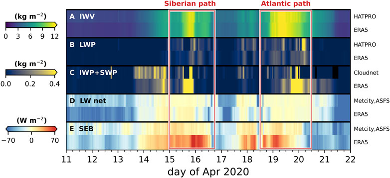
FIGURE 3. Comparison between observed and ERA5-extracted cloud and moisture parameters at RV Polarstern during mid-April 2020. The red boxes denote the peak time periods of the two subsequent episodes of the WAI, with their Siberian and Atlantic pathways. Shown are the hourly means of (A) IWV from HATPRO, (B) LWP from HATPRO, (C) IWP+SWP based on Cloudnet observations, (D) longwave net radiation (LW_net) from measurements at Met City and autonomous Atmospheric Surface Flux Stations (ASFS), (E) SEB, derived at Met City and ASFS. For LW_net and the SEB, downward fluxes are defined as positive. Included in each graph is also the ERA5 reference. Data sources are indicated on the right side.

As discussed above, the air mass origin for the two consecutive intrusions differs quite remarkably (see Section 3.1). To provide more detailed insight, 5-day backward trajectories are calculated (Supplementary Figure S2). Figure 4A shows the median latitude that air parcels resided at in the previous 5 days before arriving at RV Polarstern in different altitudes. During the background period of 11–13 April, air masses at all altitudes are of Arctic origin (lat_med ≧ 70°N). On 14 April, this slowly changes. At first, only air masses at high altitudes (approx. 7 km–11 km above ground) originate from the mid-latitudes, with median latitudes within the previous 5 days partly below 45°N. With every additional hour, starting from the top of the troposphere, more air masses also at lower altitudes stem from the mid-latitudes. This reflects typical behavior of warm fronts. On 16 April at 0 UTC, the whole atmospheric column above RV Polarstern originates from latitudes below 50°N within the past 5 days. This large-scale link is disturbed on 17 April, with the arrival of more regional Arctic air masses. On 18 April, with the onset of the intrusion from the Atlantic pathway, a new link to lower latitudes is established, starting again at higher altitudes. As this second intrusion begins to recede on 20 April, some links to lower latitudes persist at medium to high altitudes.

FIGURE 4

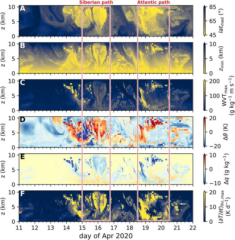
FIGURE 4. Characteristics of 5-day backward trajectories based on ERA5 starting at RV Polarstern for altitudes from the surface up to 10 km, mid-April 2020. Shown are (A) median latitude that the air masses occupied in the previous 5 days, (B) the lowest altitude at which air masses had resided, (C) maximum water vapor transport, (D) maximum change of potential temperature θ with respect to the final state, (E) maximum change of specific humidity q with respect to the state, and (F) maximum temperature tendency due to latent heat release during cloud formation.

To investigate the vertical movement of air masses, Figure 4B depicts the minimum altitude that air parcels occupied in the prior 5 days. During the pre-WAI background period, air masses typically remain relatively close to their arrival height throughout their 5-day drift, which implies the absence of strong vertical displacement. With the arrival of mid-latitude air masses around 14 April, this pattern abruptly changes. Some air parcels observed at 8 km–9 km above RV Polarstern originate close to the surface, i.e., they ascended 8 km–9 km within 5 days. Interestingly, some of these ascended air parcels previously contributed strongly to water vapor transport within the WAI (Figure 4C). In fact, the most extreme values for water vapor transport occur for air masses ending at high altitudes above the MOSAiC site (z>6 km; 14 April, 0–24 UTC and from 18 April, 12 UTC to 19 April, 24 UTC). These are altitudes at which MOSAiC radiosondes observe only very little water vapor (Supplementary Figure S3). This highlights the dynamic nature of WAIs, where air masses constantly enter and exit the corridor of moisture transport convergence.

To further study key mechanisms during air mass transport as related to thermodynamics, the maximum changes of potential temperature (Δθ) and specific humidity (Δq) along trajectories with respect to the final state at RV Polarstern are traced (Figures 4D, E). Generally, air masses arriving in the Arctic are dominantly subjected to diabatic cooling (Δθ<0 K), mostly via longwave radiation (not shown). This pattern is broken for the strongly ascending air masses, where diabatic heating dominates (Δθ>0 K), and extreme Δθ up to +20 K in 5 days are found. Here, a strong loss of water vapor occurred (Δq partly below −10 g kg^-1). This triggered intense latent heat release during cloud formation (Figure 4F), causing the extreme diabatic heating. Such heated air parcels show elevated buoyancy and therefore a greatly accelerated further ascent with or without the presence of a polar dome (Komatsu et al., 2018). In our case, this allowed some air masses to ascend over the steep Greenland orography before reaching the central Arctic (now shown). Furthermore, the lifting and moist-diabatic heating introduces negative potential vorticity anomalies to upper tropospheric levels, a fundamental prerequisite for atmospheric blocking and therefore WAI formation (You et al., 2021; 2022; Murto et al., 2022). Lifting typically occurs 1–6 days before blocking formation in rising branches of mid-latitude cyclones, often over the Atlantic basin. Our values for Δθ and Δq both roughly equal the upper 90th climatological percentile as reported by Murto et al. (2022) for the 50 most extreme high-Arctic wintertime WAIs 1979–2016. Similarly, we also detect the ascent region in close vicinity to Atlantic cyclones south of Greenland (not shown), and likewise find two subsequent warm extremes in short succession, which can be caused by a single blocking. Finally, in contrast to the strongly ascending air masses, the air arriving at RV Polarstern near the surface (z<3 km) typically experienced slight moistening and only medium water vapor transport and continuous longwave cooling on their path northwards.

To summarize this chapter, the observed double-episode WAI impacts not only the lowest layers of the Arctic atmosphere, but leaves its fingerprints on air masses reaching up to 10 km. Thus, the whole troposphere is influenced by the intrusion (Figure 4, Supplementary Figure S3A).

3.3 Air mass transformation

In this section, the evolution of the air mass along its poleward trajectory is analyzed, with focus on cloud formation and development. To estimate the role of two key cloud-determining factors, namely, CCN concentration and moisture availability, we set up dedicated LES and ICON-LAM simulation experiments (Section 2.6). In the following detailed analysis, we focus on the 19 April episode with the Atlantic pathway, centered around 12 UTC. This second intrusion peak is chosen because i) it is characterized by high temperature and moisture extremes (Supplementary Figure S3), ii) it has not been analyzed yet in the literature, and iii) it follows the climatologically more common pathway into the Arctic (as shown in Figure 2).

Figure 5A shows the temporal development of ensemble-averaged cloud LWC and IWC profiles along the trajectories (LAGRANTO calculations based on ERA5 input). In order to indicate environmental boundary conditions, the sea-ice concentration as well as the assumed clear-sky downward solar radiation are additionally depicted at the bottom and top of the graph, respectively. 16 h before encountering RV Polarstern, over the marginal sea ice zone, large amounts of liquid clouds start to form. 12 h–18 h after encountering RV Polarstern, the thick liquid cloud splits into two decks, which hints towards internal decoupling. A comparison with the cloud observations at RV Polarstern (Figure 5C) shows that the ERA5 structure of a low-level liquid-water containing cloud topped by a high-level ice cloud is realistic.

FIGURE 5

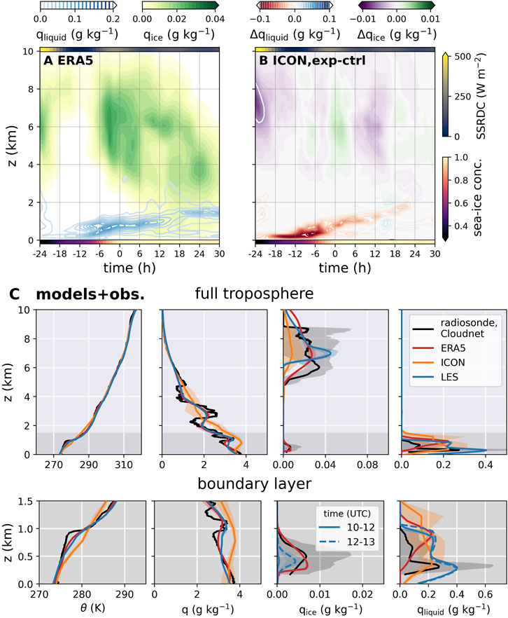
FIGURE 5. (A,B) Height-time cross sections of LWC (q_liquid, in blue) and IWC (q_ice, in green) along trajectories covering 24 h backward and 30 h forward with time. t = 0 h references 19 April 2020, 12 UTC, at RV Polarstern. Colored line at top of graphs: ERA5-based surface shortwave downward radiation under clear-sky conditions (SSRDC), colored line at bottom of graphs: ERA5-based sea-ice concentration. (A) LWC and IWC along the air mass trajectories based on ERA5, (B) LWC and IWC differences “EXP—CTRL” based on ICON-LAM. (C) Vertical thermodynamic and cloud profiles simulated and observed at RV Polarstern on 19 April, averaged for 10–12 UTC. Shown are the outputs from ERA5, control runs of the process models (LES, ICON-LAM) as well as observations from Cloudnet and radiosonde (launched at 11 UTC). Upper panel: profile covering altitudes of 0 km–10 km, bottom panel: zoomed into lowest levels covering 0 km–1.5 km.

Cloud processes critically depend on moisture availability, and therefore a targeted sensitivity experiment (EXP) with ICON-LAM is set up, where the lateral moisture inflow is reduced by up to 30% (see Section 2.6; Supplementary Figure S1). The calculations with LAGRANTO based on the ICON-LAM output show that the control run (CTRL) reflects the general observed cloud structure (Figure 5C). However, we recognize some differences in the boundary layer, at least for the snapshot around 10–12 UTC. Compared to radiosondes, the model in the lowest ca. 1 km is slightly warmer and moister. We also see differences between the simulated cloud ice content and Cloudnet observations in the boundary layer. These mainly stem from the fact that the model output represents the ice only, while the observations represent the combined ice and snow water. But importantly, the cloud liquid water is simulated realistically by ICON (Figure 5C, Supplementary Figure S3B), and this is the key for the cloud radiative effect, which we discuss in Section 3.4.

Next, the focus is set on the sensitivity of the ICON simulations. The drier atmosphere in EXP naturally generates higher surface moisture fluxes (Section 3.4), serving to mitigate the perturbation. Still, all the way from the ocean to the marginal sea ice zone, the formation of liquid water and ice clouds is strongly delayed in EXP vs. CTRL (Figure 5B). Even more notably, during the drift further into the central Arctic (t>0 h, north of RV Polarstern), similar or shortly even higher cloud water contents are found in the reduced moisture EXP. This occurs because in EXP lower temperatures are required for the air masses temperature to significantly drop below the dew point, and these temperatures are only encountered later during the poleward drift, over sea ice. Here, the CTRL clouds have already experienced significant moisture loss via precipitation (see Section 3.4)–a process that takes place later in EXP. Overall, this shift in timing leads to a rather counterintuitive result: While the higher moisture influx of CTRL features much higher cloud water contents over the ocean and marginal sea ice zone, strong precipitation formation over these regions leads to a central Arctic state where the cloud LWC is comparable between CTRL and EXP. Crucially, LWP values larger than 30 g m^-2, typically associated with a radiatively opaque state and saturated longwave cloud radiative forcing (Shupe et al., 2022), are maintained for both simulations for the initial 24 h drift into the central Arctic beyond RV Polarstern. The implications of this finding for the SEB will be discussed in Section 3.4.1.

A further factor that strongly impacts cloud formation is the availability of CCNs, a process that is investigated using Lagrangian LES experiments with the DALES model (Section 2.6). The simulations are initialized upstream of RV Polarstern at 0 UTC on 19 April. Following the low-level flow of air masses, the simulated domain arrives at RV Polarstern at 11 UTC, timed to coincide with a radiosonde launch. Figure 6A depicts the cloud LWC and IWC of the control simulations, using an initial N_CCN of 100 cm^-3. During the approach to the MOSAiC site, a well-defined low-level stratocumulus cloud layer develops. This cloud layer is predominantly of liquid phase, due to the unusually high near-surface air temperatures. At higher altitudes, a relatively thick ice layer is present. The comparison to Figure 5A illustrates that this simulated cloud structure resembles that of ERA5 along the trajectory, which is expected since ERA5 is used to force the LES. At RV Polarstern, the LES captures the observed overall cloud structure (Figure 5C). The liquid-water cloud layer constantly deepens during the air mass drift and later develops a double peak in liquid water similar to the Cloudnet observations.

FIGURE 6

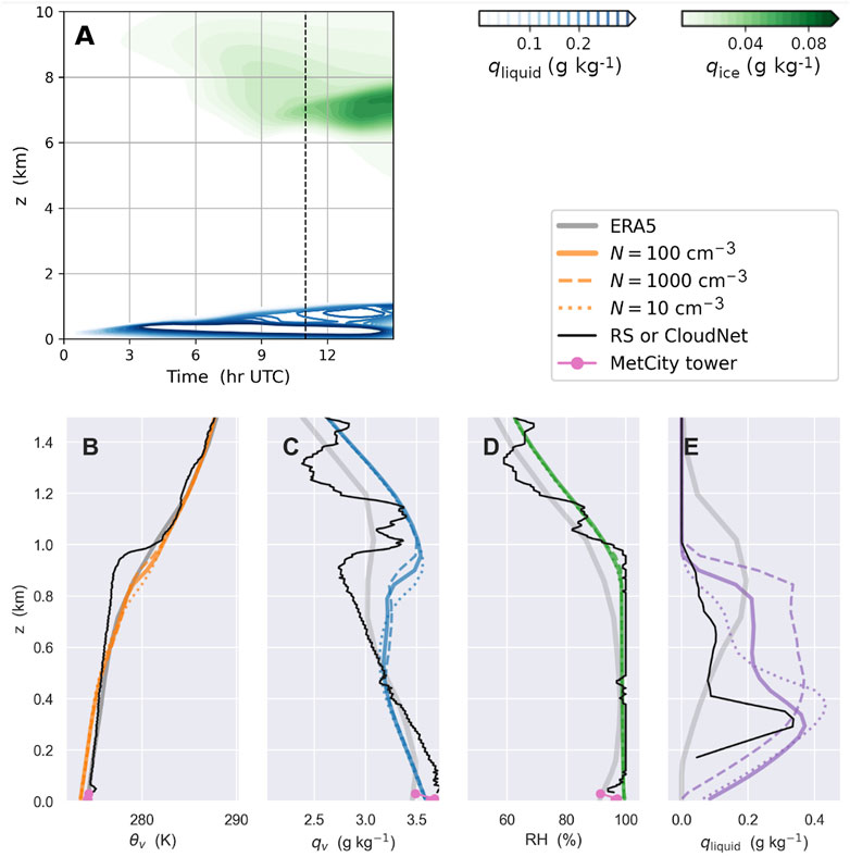
FIGURE 6. Results from Lagrangian LES simulations with the DALES code for 19 April 2020. Upper panel: (A) Height-time cross sections of cloud LWC (q_liquid, in blue) and IWC (q_ice, in green). The dashed black line at 11 UTC indicates the air mass arrival time at RV Polarstern. Lower panels: Domain-averaged thermodynamic profiles at 11 UTC of (B) virtual potential temperature θ_v, (C) water vapor specific humidity q_v, (D) relative humidity RH and (E) cloud liquid water specific humidity q_liquid. Three LES experiments are shown in orange, with N indicating the initial CCN concentration in cm^-3 (dashed, solid and dotted). The radiosonde (RS) and Cloudnet data are shown in black, the 10 m Met Tower data in pink, and ERA5 in gray.

In addition to the control simulation, two sensitivity experiments are performed, in which the initial CCN concentration N_CCN is altered (Figures 6B–E). One reflects pristine Arctic conditions (N_CCN = 10 cm^-3), the other represents the polluted continental concentrations observed at RV Polarstern during this period (N_CCN = 1,000 cm^-3; Dada et al., 2022). This range reflects the observed variation during the selected days, and thus guides the sensitivity experiment. With the basic observed boundary-layer state already reproduced to a reasonable degree in the control experiment, thus one single aspect (the CCN concentration) is varied in a virtual laboratory setting, to assess its impact while keeping all other factors constant. In doing so, it is possible to gain insight into how the CCN concentration can affect the boundary layer structure on its way to RV Polarstern. When interpreting the outcome of the sensitivity test, it should be considered that the imposed large-scale forcings and boundary conditions still carry significant uncertainty, mainly due to a lack of measurements in upstream areas. We thus do not seek perfect agreement with the observations at RV Polarstern; instead, the main goal is to understand impacts, given the observed CCN range.

Several things can be noted by comparing the different LES runs. The impact of CCN concentrations on the boundary layer, in particular on the inversion height, is evident. The polluted air masses feature a slightly deeper boundary layer, exceeding that of the pristine simulation by approximately 100 m and agreeing best with the radiosonde data. The vertical structure and amount of the low-level liquid water clouds changes substantially as well, such that more liquid water occurs at the top part of the cloud in the polluted simulation. The interrelated mechanisms that take place works as follows: With larger N_CCN, the cloud LWC increases. Accordingly, increased longwave cooling at the (now sharper) cloud top makes radiatively driven entrainment more efficient and deepens the boundary layer (Stevens et al., 2005). The intensified entrainment warming partially counteracts the cloud top cooling. These presented mechanisms align well with the findings of Chylik et al. (2021) who employed a LES on a case observed during the ACLOUD field campaign in the Fram Strait (Wendisch et al., 2019).

According to our simulations, this mechanism may also play a role in air mass transformation during WAIs, and may impact the lifetime of cloudy air masses through modification of precipitation. It moreover highlights that accurate observations of N_CCN are needed for realistic model simulations of cloud processes in WAIs.

Another finding is the importance of correctly assed cooling rates. The zoom-in to the boundary layer in Figure 5C compares results using data that is extended from the original 10–12 UTC time window to 12–13 UTC. By allowing the air mass to drift and cool just 1 h longer, sufficient cooling triggers the formation of a low-level mixed phase cloud with q_ice>0 g kg^-1. This is better in line with the Cloudnet observations, which also show a mixed-phase cloud instead of a pure liquid-phase cloud.

3.4 Surface impact

3.4.1 Surface energy budget

The aforementioned cloud changes during the air mass transformation along the WAI path are expected to impact the SEB, which we further discuss in this section. We continue our focus on the 19 April episode. To directly attribute changes in SEB to the intrusion, we again apply the Lagrangian approach and examine the SEB components from ERA5 along the calculated air mass trajectories. We define the SEB as the sum of the radiative and turbulent heat fluxes. Fluxes towards the surface are defined as positive, i.e., warming the surface.

Figure 7A shows the ERA5-LAGRANTO-derived components of the SEB along the trajectory, as well as environmental conditions (sea-ice concentration, surface downward solar radiation under clear sky assumption). In the 24 h preceding its arrival above RV Polarstern, the air mass traverses the ocean and marginal sea ice zone to the east of Greenland, eventually reaching the consolidated ice pack (Supplementary Figures S1, S2). Strongly positive daytime values of the SEB of above +200 W m^-2 and strong sensible heat fluxes from the atmosphere to the surface of up to + 50 W m^-2 are found. The surface net cloud radiative forcing (CRF) is strongly negative as large as −100 W m^-2, indicating a cooling effect of clouds over the ocean and marginal sea ice zone, in part because of the high shortwave radiation at this time of day. CRF is mediated by thick ice clouds, as liquid-water containing clouds are still mostly absent (see Figure 5A). Furthermore, the absence of liquid cloud water correlates with negligible longwave CRF (i.e., warming) and allows for an efficient surface radiative cooling.

FIGURE 7

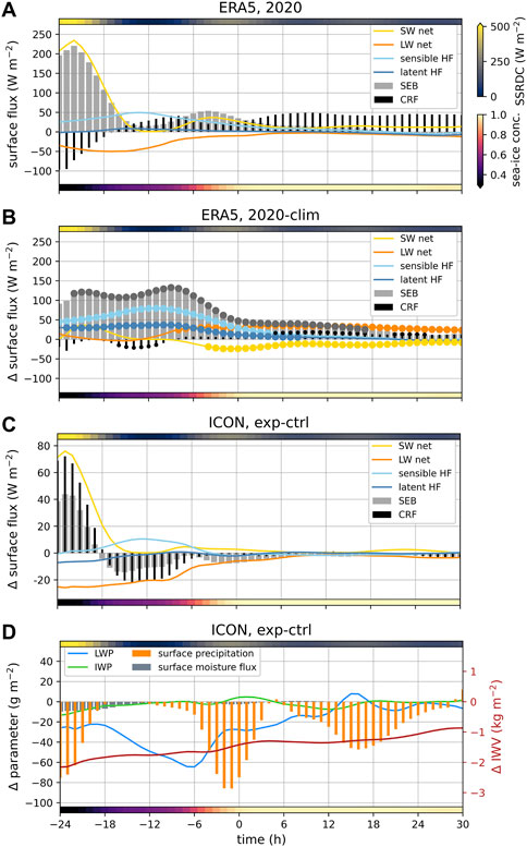
FIGURE 7. (A–C) Time series of the SEB and its components (net short- and longwave SW and LW, sensible and latent heat fluxes HF), as well as CRF along trajectories. At the top of each graph, ERA5-based surface shortwave downward radiation under clear-sky conditions (SSRDC) is depicted. At the bottom of each graph, ERA5-based sea-ice concentration is shown. Time is relative to 19 April, 12 UTC. (A) ERA5 reanalysis, 2020 event (B) Difference of 2020 WAI minus 1979–2020 climatology, based on ERA5. Dots indicate timesteps where surface fluxes exceed one climatological standard deviation. (C) Differences EXP-CTRL based on ICON-LAM simulations. (D) As in (C) but for LWP and IWP, IWV, surface precipitation and surface moisture flux.

During the course of the next few days with cloud formation and the track over the ice, turbulent heat fluxes decrease. CRF is now exclusively positive in the range from +25 W m⁻² to +50 W m⁻² (warming longwave CRF), with slightly reduced values during daytime (cooling shortwave CRF). The longwave net radiation rises to around 0 W m⁻², indicating that strong downward longwave fluxes cancel the upward-directed longwave cooling. The resulting net SEB decreases to values around 0 W m⁻².

Comparing the event to the 1979–2020 climatology along the drift pathway, shown in Figure 7B, we find that the WAI’s impact on the SEB is an overall anomalous warming. However, the main contributions and the absolute effect varies with the surface type. This agrees with other recent studies (e.g., Murto et al., 2022; You et al., 2022). Over open ocean and in the marginal sea ice zone, both latent and sensible heat fluxes are significantly higher than the climatological averages. The WAI leads to a SEB anomaly of up to +140 W m⁻². Over sea ice, the anomalies of all four SEB components are reduced, resulting in a SEB anomaly of only about +50 W m⁻². The contributions of both latent and sensible heat flux are less important in this region, while the longwave radiation anomaly plays a larger role and shows a positive anomaly, i.e., less net longwave radiation loss from the surface happens during the WAI. This is counteracted by a comparable negative shortwave radiation anomaly. Both radiative effects are consistent with enhanced cloud influences during the WAI (Section 3.3, and e.g., Clancy et al., 2022; Finocchio and Doyle, 2021), and the warming CRF effect dominates. Deeper in the central Arctic (t>24 h beyond Polarstern), the short- and longwave contributions add up to only a small anomalous SEB of +20 W m⁻² and the net CRF anomaly remains positive, but small. Overall, the anomalies of SEB components during the mid-April 2020 event are within the order of magnitude as reported for WAIs in other seasons (recently e.g., Murto et al., 2022; Bresson et al., 2022; You et al., 2022). Furthermore, our reported WAI-related SEB anomalies are consistent with surface energy flux anomalies associated with cyclones and related sea-ice changes (recently, Aue et al., 2022; Clancy et al., 2022; Finoccio et al., 2022).

To better understand the influence of advected atmospheric moisture during this event, we explore the ICON-LAM experiments (Section 2.6). Figure 7C shows the difference of the “SEB in EXP with reduced moisture inflow minus CTRL” along the trajectory. The general ability of the ICON-LAM control run to represent the observed SEB during this WAI can be seen in Supplementary Figure S3B. As depicted in Figures 5B, 7D, the reduced moisture inflow results in reduced cloud LWC and IWC. Therefore, at the lower latitudes in the first 6 h of the drift, the shortwave radiation is not blocked as much and is up to +70 W m⁻² higher than in the control run. This effect is also reflected in the much more positive CRF at these time steps. Furthermore, the prevented cloud formation also allows for more energy loss via longwave radiation. This effect is especially important at the marginal sea ice zone and when the trajectory drifts through the night (negligible incoming shortwave radiation). Here, the CRF is about 20 W m⁻² lower than in the control run. These radiative processes result in a slightly colder surface, which then increases the surface sensible heat flux relative to the control run. The latent heat flux only changes over the open ocean due to an increased thermodynamically-driven evaporation. After entering the central Arctic, the difference EXP-CTRL is only minimal, i.e., similar SEBs are found for both simulations. For EXP as well as CTRL, LWP values larger than 30 g m⁻² and thus near-saturated longwave CRF persist into the inner Arctic. Additionally, CTRL has already lost significant amounts of cloud water through precipitation over the ocean and the marginal sea ice zone (Figure 7D), while EXP is able to conserve its cloud water for a longer time. Hence the difference of LWP values narrows.

Overall, the model experiments imply that WAIs with reduced moisture inflow can cause an elevated SEB in the daytime over ocean, but a lowered SEB later when passing the marginal sea ice zone during nighttime, compared to more intense (moister) WAI. Interestingly, as long as a near-saturation of longwave CRF is achieved, for an initially drier WAI the impact on the SEB over the ice-covered central Arctic Ocean might be quite comparable.

3.4.2 Precipitation and snowfall

The time series of hourly snowfall rates at RV Polarstern shows that the mid-April 2020 double-episode WAI event brought considerable amounts of snowfall to the MOSAiC site (Figure 8A). During the first episode (15–16 April), the different measurement platforms observe snowfall rates up to 2 mm h⁻¹. From 16 April noon to 19 April noon, only little precipitation is recorded. Then, on 20 April the precipitation rate increases up to values of 2.5 mm h⁻¹. The figure also highlights the high uncertainty of snowfall estimates. Particularly during the second episode on 20 April, the snowfall rates derived from reanalysis data, satellite and ground-based measurements strongly vary. The temporal evolution of the snowfall rate from ERA5 reanalysis agrees relatively well with the ground-based measurements (KAZR, Pluvio), but shows a tendency to slightly underestimate the snowfall. The snowfall rate estimated from satellites can deviate by up to a factor of two. This deviation can partially be attributed to the fact that the precipitation rates spatially vary significantly across the domain around RV Polarstern, resulting in different precipitation values for the nearest satellite pixels. Moreover, such small-scale variability has an impact on the satellite estimates especially for the large ATMS pixel sizes (viewing angles > 20°) encountered at RV Polarstern’s position. Here, the spatial resolution reduces from 16 × 16 km² at nadir down to 68 × 30 km² at the edges (Weng et al., 2012). Still, the good skill of SLALOM-CT especially on 16 and 19 April warrants further future assessment of this novel algorithm.

FIGURE 8

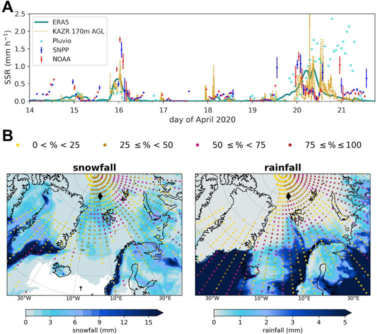
FIGURE 8. (A) Time series of the surface snowfall rate (SSR) at RV Polarstern during the peak intrusion period, from 14 April, 0 UTC until 21 April, 23 UTC. For ERA5 (cyan solid line) the grid cell closest to RV Polarstern position is taken. For satellite ATMS measurements (NOAA-20: red points, SNPP: blue points), SLALOM-CT estimates at RV Polarstern nearest pixel and standard deviations on a 3 × 3 pixel window are shown. In addition, ground-based measurements (Pluvio - turquoise points, KAZR at 170 m above ground - yellow dashed line) are shown. (B) Snowfall (left), and rainfall (right) accumulated for the 9-day period mentioned in (A), based on ERA5. The colored dots illustrate the contribution of the two intense episodes of the WAI to precipitation as detected via the atmospheric river algorithm during that time period. The location of RV Polarstern is marked by the black diamond.

Next, precipitation patterns based on ERA5 are investigated on a larger spatial scale. The fraction of precipitation (rain, snow), as directly caused by the WAIs is calculated based on the atmospheric river shape (Section 2.4; Figure 8B). In the slightly shorter mid-April period considered here (14–22 April), the total 9-day snowfall and rainfall are calculated for each grid cell individually. Then, the fraction of precipitation deposited by the detected atmospheric river is extracted. We find that the atmospheric river components of the WAI contribute about 30% to the total precipitation (27% snowfall, 3% rainfall) at the grid cell nearest to RV Polarstern. A similar magnitude of contribution was calculated during two other campaigns in the Arctic (Lauer et al., 2023). Even larger fractions are discovered further east and south, at the marginal sea ice zone. However, it should be stressed that the exact contribution percentages depend on the detection algorithm applied, and might thus vary for different algorithms (Viceto et al., 2022).

The high uncertainty of precipitation estimates has important consequences. As demonstrated, WAIs bring large amounts of rain and snowfall into the central Arctic. These can have major impacts on the sea ice, such as increased insulation (snow on sea ice), modified surface albedo, or altered mass balance. Depending on the season, this can heavily influence longwave cooling efficiency and shortwave surface heating, and thus SEB and sea-ice cover.

4 Summary and conclusion

In our detailed analysis of the record-breaking WAI observed in mid-April 2020 during the MOSAiC expedition, we come to the following conclusion, according to our three objectives:

• (O1) Synoptic situation and transport: The WAI is characterized by two distinct pathways (Siberian, Atlantic) and exceptional moist static energy transports above the 90th percentile of climatology. The strongest anomaly is found in the latent energy transport along the Siberian pathway. This anomalous moisture transport is driven by a persistent positive NAO and later by a Scandinavian blocking pattern. Air masses at all altitudes between the surface and 10 km feature mid-latitude origins with median latitudes during the 5 previous days of 45°N and below.

• (O2) Air mass transformation via cloud processes: As measured at the MOSAiC site, the WAI establishes low-level liquid water and high-level ice clouds in the central Arctic. The observed LWP larger than 30 g m⁻² is typically associated with the radiatively opaque state of the Arctic atmosphere. Model experiments demonstrate that two key cloud-determining factors, namely, moisture inflow and CCN concentration, can significantly affect the vertical cloud structure and especially the amount of the low-level liquid clouds. In the simulations, a reduction of both factors causes a reduction of LWC at the MOSAiC site. Furthermore, we show how modifications in CCN concentrations can trigger complex cloud-boundary layer feedbacks: Higher CCN concentrations lead to higher LWC in low-level liquid clouds and an associated stronger longwave cloud-top cooling. This leads to stronger entrainment and thus a stronger mixing in the boundary layer.

• (O3) Surface impacts: Along the poleward drift, the WAI has a strong and anomalous warming influence on the SEB. It is mostly driven by turbulent heat fluxes over the ocean and by radiation (longwave radiation, cloud radiative forcing) over the sea ice. For a reduced moisture inflow, major SEB impacts are mainly seen at the beginning of the track over the ocean and the marginal sea ice zone, but not the inner Arctic. The WAI contributes to a large, regionally variable fraction in total precipitation over a 9-day period, reaching up to about 30% at the MOSAiC site. We stress the pronounced uncertainty in precipitation and specifically snowfall observational estimates.

With these new insights, follow-up research is emerging. In the future, additional dedicated model experiments can help to further address the (O2) objective touched on here, namely, to better understand how complex aerosol-cloud-precipitation processes affect air mass transformation. For example, further exploration of processes is needed that are involved in controlling the moisture content of air masses. The simulations conducted here suggest counter-intuitive responses of the air mass to reduced moisture content, and further studies are needed to explore the responses and potential thresholds related to the amount of moisture in WAIs. The role of CCN in these processes also warrants further study. To first order, increased CCN should decrease the precipitation efficiency of an air mass, however it is not clear if, or how, such pollution impacts the cloudiness along the trajectory, the rate at which moisture is removed, or the implications for the SEB (O3). The analysis of the relationship between WAIs and sea-ice concentration is complicated as well and calls for follow-up research. No significant reduction of sea ice concentration is reported during mid-April 2020 from the ship during MOSAiC (Krumpen et al., 2021), but false, too low passive microwave satellite sea-ice concentration retrievals due to weather and surface glazing effects (Schreiber and Serreze, 2020) make interpretation difficult (Krumpen et al., 2021). We manually inspected synthetic aperture radar satellite scenes, which are less contaminated by weather influence, and can confirm that some leads opened and closed during the WAI, but sea ice concentration in the vicinity of RV Polarstern stayed high (> 95%). Overall, more in-depth studies are needed to separate retrieval uncertainties from actual sea ice changes and to further divide the latter into dynamic and thermodynamic components.

Finally, we stress that we present results for a specific case study only. It will be informative to extend some of our methods to climatological data sets in order to substantiate the robustness of our findings.

Data availability statement

Publicly available datasets were analyzed in this study. This data can be found here: MOSAiC meteorological data from Met City and the ASFS are available at the Arctic Data Center (Cox et al. 2021a, b, c, d). Radiation data from Met City (Riihimaki, 2022), Pluvio data (Cromwell and Bartholomew, 2022), and KAZR-based snowfall data (Matrosov et al., 2022) are available from the DOE ARM Archive. IWV and LWP as derived from HATPRO (Walbröl et al., 2022) as well as radiosonde data are freely available at PANGEA: https://doi.pangaea.de/10.1594/PANGAEA.941389, https://doi.org/10.1594/PANGAEA.928656. All data related to reanalysis can be found on the ERA5 data repository: https://www.ecmwf.int/en/forecasts/dataset/ecmwf-reanalysis-v5 (last access: 12 January 2023; Hersbach et al., 2020). The main outputs of LES experiments are available at: https://doi.org/10.5281/zenodo.7544108, while the current version of DALES (dales 4.3 with extension for mixed-phase microphysics, https://doi.org/10.5281/zenodo.5642477) is available on github as https://github.com/jchylik/dales/releases/tag/dales4.3sb3cgn. Lastly, the following data is available by contacting the lead author: SLALOM-CT estimates of surface snowfall; mean sea-level pressure fields of ICON-CTRL; cloud liquid and ice water contents along trajectories based on ERA5, ICON-CTRL and ICON-EXP.

Author contributions

AR, BK, RN, SC, and ST contributed to conception and design of the study. Observational data was supplied and interpretation supported by: AC (SLALOM-CT), AR and MS (SEB components, KAZR), AW (HATPRO), HG (Cloudnet). BK performed synoptic analysis based on ERA5, trajectory calculations based on ERA5 and ICON-LAM, and created most figures. IH and DH investigated preferred circulation regimes and large-scale energy transport. ML compared precipitation estimates from different platforms and weather systems, applying the atmospheric river algorithm. RN and JC performed and analyzed LES simulations. ST performed ICON-LAM simulations and analyzed them together with BK. BK, AR, and ST wrote the first draft of the article. BK coordinated the co-author’s input. AR, BK, IH, ML, RN, and ST wrote sections of the manuscript. All authors actively discussed the draft, contributed to manuscript revision and approved the submitted version.

Funding

We acknowledge funding by the Deutsche Forschungsgemeinschaft (DFG, German Research Foundation)— project 268020496 TRR 172, within the Transregional Collaborative Research Center “ArctiC Amplification: Climate Relevant Atmospheric and SurfaCe Processes, and Feedback Mechanisms (AC)³”. MS acknowledges support of a Mercator Fellowship as part of (AC)³, the National Science Foundation (OPP-1724551), and the NOAA Global Ocean Monitoring and Observing Program (via NA22OAR4320151). AR and DH were partly supported by the European Union’s Horizon 2020 research and innovation framework programme under Grant agreement no. 101003590 (PolarRES). IG thanks FCT/MCTES for financial support to CESAM (UIDP/50017/2020, UIDB/50017/2020, and LA/P/0094/2020), to CIIMAR (UIDB/04423/2020, UIDP/04423/2020) and individual funding 2021.03140.CEECIND through national funds provided by FCT—Fundação para a Ciência e a Tecnologia. Data was collected from the Multidisciplinary drifting Observatory for the Study of the Arctic Climate (MOSAiC) under expedition number MOSAiC20192020 and project identifying AWI_PS122_00. The Gauss Centre for Supercomputing e.V., (www.gauss-centre.eu) is acknowledged for providing computing time on the GCS Supercomputer JUWELS at the Jülich Supercomputing Centre (JSC) under project VIRTUALLAB.The publication of this article was funded by the Open Access Publishing Fund of Leipzig University, supported by the German Research Foundation within the program Open Access Publication Funding.

Acknowledgments

Data was collected from the Multidisciplinary drifting Observatory for the Study of the Arctic Climate (MOSAiC). Some data was obtained from the Atmospheric Radiation Measurement (ARM) User Facility, a U.S. Department of Energy Office (DOE) of Science User Facility managed by the Biological and Environmental Research Program.

Conflict of interest

The authors declare that the research was conducted in the absence of any commercial or financial relationships that could be construed as a potential conflict of interest.

Publisher’s note

All claims expressed in this article are solely those of the authors and do not necessarily represent those of their affiliated organizations, or those of the publisher, the editors and the reviewers. Any product that may be evaluated in this article, or claim that may be made by its manufacturer, is not guaranteed or endorsed by the publisher.

Supplementary material

The Supplementary Material for this article can be found online at: https://www.frontiersin.org/articles/10.3389/feart.2023.1147848/full#supplementary-material

References

Ali, S. M., and Pithan, F. (2020). Following moist intrusions into the Arctic using SHEBA observations in a Lagrangian perspective. Q. J. R. Meteorol. Soc. 146, 3522–3533. doi:10.1002/qj.3859

CrossRef Full Text | Google Scholar

Aue, L., Vihma, T., Uotila, P., and Rinke, A. (2022). New insights into cyclone impacts on sea ice in the Atlantic sector of the Arctic Ocean in winter. Geophys. Res. Lett. 49, e2022GL100051. doi:10.1029/2022GL100051

CrossRef Full Text | Google Scholar

Batrak, Y., and Müller, M. (2019). On the warm bias in atmospheric reanalyses induced by the missing snow over Arctic sea-ice. Nat. Commun. 10, 4170. doi:10.1038/s41467-019-11975-3

PubMed Abstract | CrossRef Full Text | Google Scholar

Bechtold, P., Köhler, M., Jung, T., Doblas-Reyes, F., Leutbecher, M., Rodwell, M. J., et al. (2008). Advances in simulating atmospheric variability with the ECMWF model: From synoptic to decadal time-scales. Q. J. R. Meteorol. Soc. 134 (634), 1337–1351. doi:10.1002/qj.289

CrossRef Full Text | Google Scholar

Binder, H., Boettcher, M., Grams, C. M., Joos, H., Pfahl, S., and Wernli, H. (2017). Exceptional air mass transport and dynamical drivers of an extreme wintertime Arctic warm event. Geophys. Res. Lett. 44, 12028–12036. doi:10.1002/2017gl075841

CrossRef Full Text | Google Scholar

Boisvert, L. N., Petty, A. A., and Stroeve, J. C. (2016). The impact of the extreme winter 2015/16 Arctic cyclone on the Barents–Kara seas. Mon. Wea. Rev. 144, 4279–4287. doi:10.1175/mwr-d-16-0234.1

CrossRef Full Text | Google Scholar

Bresson, H., Rinke, A., Mech, M., Reinert, D., Schemann, V., Ebell, K., et al. (2022). Case study of a moisture intrusion over the arctic with the ICOsahedral non-hydrostatic (ICON) model: Resolution dependence of its representation. Atmos. Chem. Phys. 22, 173–196. doi:10.5194/acp-22-173-2022

CrossRef Full Text | Google Scholar

Bretherton, C. S., Krueger, S. K., Wyant, M. C., Bechtold, P., Van Meijgaard, E., Stevens, B., et al. (1999). A GCSS boundary-layer cloud model intercomparison study of the first ASTEX Lagrangian experiment. Boundary-Layer Meteorol. 93, 341–380. doi:10.1023/A:1002005429969

CrossRef Full Text | Google Scholar

Bretherton, C. S., Uchida, J., and Blossey, P. N. (2010). Slow manifolds and multiple equilibria in stratocumulus-capped boundary layers. J. Adv. Model. Earth Syst. 2 (14). doi:10.3894/JAMES.2010.2.14

CrossRef Full Text | Google Scholar

Camplani, A., Casella, D., Sanò, P., and Panegrossi, G. (2021). The passive microwave empirical cold surface classification algorithm (PESCA): Application to GMI and ATMS. J. Hydrometeorol. 22 (7), 1727–1744. doi:10.1175/jhm-d-20-0260.1

CrossRef Full Text | Google Scholar

Chylik, J., Chechin, D., Dupuy, R., Kulla, B. S., Lüpkes, C., Mertes, S., et al. (2021). Aerosol-cloud-turbulence interactions in well-coupled Arctic boundary layers over open water. Atmos. Chem. Phys. Discuss. [Preprint]. doi:10.5194/acp-2021-888

CrossRef Full Text | Google Scholar

Clancy, R., Bitz, C. M., Blanchard-Wrigglesworth, E., McGraw, M. C., and Cavallo, S. M. (2022). A cyclone-centered perspective on the drivers of asymmetric patterns in the atmosphere and sea ice during Arctic cyclones. J. Clim. 35 (1), 1–47. doi:10.1175/jcli-d-21-0093.1

CrossRef Full Text | Google Scholar

Cox, C., Gallagher, M., Shupe, M., Persson, O., Solomon, A., Ayers, T., et al. (2021b). Atmospheric surface flux station #30 measurements (level 1 raw), Multidisciplinary drifting Observatory for the Study of Arctic Climate (MOSAiC), central Arctic, October 2019 - September 2020. Alexandria, VA, United States: National Science Foundation’s Office of Polar Programs. doi:10.18739/A20C4SM1J

CrossRef Full Text | Google Scholar

Cox, C., Gallagher, M., Shupe, M., Persson, O., Solomon, A., Ayers, T., et al. (2021d). Atmospheric surface flux station #40 measurements (level 1 raw), Multidisciplinary drifting Observatory for the Study of Arctic Climate (MOSAiC), central Arctic, October 2019 - September 2020. Alexandria, VA, United States: National Science Foundation’s Office of Polar Programs. doi:10.18739/A2CJ87M7G

CrossRef Full Text | Google Scholar

Cox, C., Gallagher, M., Shupe, M., Persson, O., Solomon, A., Ayers, T., et al. (2021c). Atmospheric surface flux station #50 measurements (level 1 raw), Multidisciplinary drifting Observatory for the Study of Arctic Climate (MOSAiC), central Arctic, October 2019 - September 2020. Alexandria, VA, United States: National Science Foundation’s Office of Polar Programs. doi:10.18739/A2445HD46

CrossRef Full Text | Google Scholar

Cox, C., Gallagher, M., Shupe, M., Persson, O., Solomon, A., Blomquist, B., et al. (2021a). 10-meter (m) meteorological flux tower measurements (level 1 raw), Multidisciplinary drifting Observatory for the Study of Arctic Climate (MOSAiC), central Arctic, October 2019 - September 2020. Alexandria, VA, United States: National Science Foundation’s Office of Polar Programs. doi:10.18739/A2VM42Z5F

CrossRef Full Text | Google Scholar

Crasemann, B., Handorf, D., Jaiser, R., Dethloff, K., Nakamura, T., Ukita, J., et al. (2017). Can preferred atmospheric circulation patterns over the North-Atlantic-Eurasian region be associated with Arctic sea ice loss? Polar Sci. 14, 9–20. doi:10.1016/j.polar.2017.09.002

CrossRef Full Text | Google Scholar

Crawford, A. D., Lukovich, J. V., McCrystall, M. R., Stroeve, J. C., and Barber, D. G. (2022). Reduced sea ice enhances intensification of winter storms over the Arctic Ocean. J. Clim. 35 (11), 3353–3370. doi:10.1175/jcli-d-21-0747.1

CrossRef Full Text | Google Scholar

Cromwell, E., and Bartholomew, M. J. (2022). Weighing bucket precipitation gauge (WBPLUVIO2). Atmospheric Radiation Measurement (ARM) User Facility. doi:10.5439/1338194

CrossRef Full Text | Google Scholar

Dada, L., Angot, H., Beck, I., Baccarini, A., Quéléver, L. L. J., Boyer, M., et al. (2022). A central Arctic extreme aerosol event triggered by a warm air-mass intrusion. Nat. Commun. 13, 5290. doi:10.1038/s41467-022-32872-2

PubMed Abstract | CrossRef Full Text | Google Scholar

Dahlke, S., and Maturilli, M. (2017). Contribution of atmospheric advection to the amplified winter warming in the Arctic North Atlantic region. Adv. Meteorol. 2017, 1–8. doi:10.1155/2017/4928620

CrossRef Full Text | Google Scholar

Doms, G., Forstner, J., Heise, E., Herzog, H.-J., Mironov, D., Raschendorfer, M., et al. (2011). A description of the nonhydrostatic regional COSMO model. Part II: Physical parameterization. Consortium for small-scale modelling. Available at: http://www.cosmo-model.org.

Google Scholar

ECMWF (2020). ECMWF newsletter number 164 - summer 2020, European Centre for medium-range weather forecasts (ECMWF). Available at: https://www.ecmwf.int/en/newsletter/164/news/warm-intrusions-arctic-april-2020 (Accessed January 16, 2023).

Google Scholar

Falkena, S. K. J., Wiljes, J., Weisheimer, A., and Shepherd, T. G. (2020). Revisiting the identification of wintertime atmospheric circulation regimes in the Euro-Atlantic sector. Q. J. R. Meteorol. Soc. 146, 2801–2814. doi:10.1002/qj.3818

CrossRef Full Text | Google Scholar

Fearon, M. G., Doyle, J. D., Ryglicki, D. R., Finocchio, P. M., and Sprenger, M. (2021). The role of cyclones in moisture transport into the Arctic. Geophys. Res. Lett. 48, e2020GL090353. doi:10.1029/2020gl090353

CrossRef Full Text | Google Scholar

Finocchio, P. M., and Doyle, J. D. (2021). Summer cyclones and their association with short-term sea ice variability in the Pacific sector of the Arctic. Front. Earth Sci. 9, 738497. doi:10.3389/feart.2021.738497

CrossRef Full Text | Google Scholar

Finoccio, P. M., Doyle, J. D., and Stern, D. P. (2022). Accelerated sea ice Loss from late summer cyclones in the New Arctic. J. Clim. 35, 4151–4169. doi:10.1175/jcli-d-22-0315.1

CrossRef Full Text | Google Scholar

Graham, R. M., Cohen, L., Petty, A. A., Boisvert, L. N., Rinke, A., Hudson, S. R., et al. (2017). Increasing frequency and duration of Arctic winter warming events. Geophys. Res. Lett. 44, 6974–6983. doi:10.1002/2017gl073395

CrossRef Full Text | Google Scholar

Graham, R. M., Cohen, L., Ritzhaupt, N., Segger, B., Graversen, R. G., Rinke, A., et al. (2019a). Evaluation of six atmospheric reanalyses over Arctic sea ice from winter to early summer. J. Clim. 32, 4121–4143. doi:10.1175/jcli-d-18-0643.1

CrossRef Full Text | Google Scholar

Graham, R. M., Hudson, S. R., and Maturilli, M. (2019b). Improved performance of ERA5 in Arctic gateway relative to four global atmospheric reanalyses. Geophys. Res. Lett. 46, 6138–6147. doi:10.1029/2019gl082781

CrossRef Full Text | Google Scholar

Graversen, R. G., and Burtu, M. (2016). Arctic amplification enhanced by latent energy transport of atmospheric planetary waves. Q. J. R. Meteorol. Soc. 142, 2046–2054. doi:10.1002/qj.2802

CrossRef Full Text | Google Scholar

Guan, B., Waliser, D. E., and Ralph, F. M. (2018). An intercomparison between reanalysis and dropsonde observations of the total water vapor transport in individual atmospheric rivers. J. Hydrometeorol. 19, 321–337. doi:10.1175/JHM-D-17-0114.1

CrossRef Full Text | Google Scholar

Hannachi, A., Straus, D. M., Franzke, C. L. E., Corti, S., and Woollings, T. (2017). Low-frequency nonlinearity and regime behavior in the Northern Hemisphere extratropical atmosphere. Rev. Geophys. 55, 199–234. doi:10.1002/2015rg000509

CrossRef Full Text | Google Scholar

Henderson, G. R., Barrett, B. S., Wachowicz, L. J., Mattingly, K. S., Preece, J. R., and Mote, T. L. (2021). Local and remote atmospheric circulation drivers of Arctic change: A review. Front. Earth Sci. 9. doi:10.3389/feart.2021.709896

CrossRef Full Text | Google Scholar

Hersbach, H., Bell, B., Berrisford, P., Hirahara, S., Horányi, A., Muñoz-Sabater, J., et al. (2020). The ERA5 global reanalysis. Q. J. R. Meteorol. Soc. 146, 1999–2049. doi:10.1002/qj.3803

CrossRef Full Text | Google Scholar

Heus, T., van Heerwaarden, C. C., Jonker, H. J. J., Siebesma, A. P., Axelsen, S., van den Dries, K., et al. (2010). Formulation of the Dutch atmospheric large-eddy simulation (DALES) and overview of its applications. Geoph. Model Dev. 3, 415–444. doi:10.5194/gmd-3-415-2010

CrossRef Full Text | Google Scholar

Hogan, R. J., and Bozzo, A. (2018). A flexible and efficient radiation scheme for the ECMWF model. J. Adv. Model. Earth Syst. 10, 1990–2008. doi:10.1029/2018ms001364

CrossRef Full Text | Google Scholar

Illingworth, A. J., Hogan, R. J., O'Connor, E. J., Bouniol, D., Brooks, M. E., Delanoé, J., et al. (2007). Cloudnet. Bull. Am. Meteorol. Soc. 88, 883–898. doi:10.1175/bams-88-6-883

CrossRef Full Text

Johansson, E., Devasthale, A., Tjernström, M., Ekman, A. M. L., and L’Ecuyer, T. (2017). Response of the lower troposphere to moisture intrusions into the Arctic. Geophys. Res. Lett. 44, 2527–2536. doi:10.1002/2017gl072687

CrossRef Full Text | Google Scholar

Komatsu, K. K., Alexeev, V. A., Repina, I. A., and Tachibana, Y. (2018). Poleward upgliding Siberian atmospheric rivers over sea ice heat up Arctic upper air. Sci. Rep. 8, 2872. doi:10.1038/s41598-018-21159-6

PubMed Abstract | CrossRef Full Text | Google Scholar

Krumpen, T., von Albedyll, L., Goessling, H., Hendricks, S., Juhls, B., Spreen, G., et al. (2021). MOSAiC drift expedition from October 2019 to July 2020: Sea ice conditions from space and comparison with previous years. Cryosphere 15, 3897–3920. doi:10.5194/tc-15-3897-2021

CrossRef Full Text | Google Scholar

Lauer, M., Rinke, A., Gorodetskaya, I., Sprenger, M., Mech, M., and Crewell, S. (2023). Influence of atmospheric rivers and associated weather systems on precipitation in the Arctic. EGUsphere. [Preprint]. doi:10.5194/egusphere-2023-261

CrossRef Full Text | Google Scholar

Lembo, V., Messori, G., Graversen, R., and Lucarini, V. (2019). Spectral decomposition and extremes of atmospheric meridional energy transport in the Northern hemisphere midlatitudes. Geophys. Res. Lett. 46, 7602–7613. doi:10.1029/2019gl082105

CrossRef Full Text | Google Scholar

Li, L., Cannon, F., Mazloff, M. R., Subramanian, A. C., Wilson, A. M., and Ralph, F. M. (2022). Impact of atmospheric rivers on Arctic sea ice variations. EGUsphere. [Preprint]. doi:10.5194/egusphere-2022-36

CrossRef Full Text | Google Scholar

Liang, Y., Bi, H., Huang, H., Lei, R., Liang, X., Cheng, B., et al. (2022). Contribution of warm and moist atmospheric flow to a record minimum July sea ice extent of the Arctic in 2020. Cryosphere 16, 1107–1123. doi:10.5194/tc-16-1107-2022

CrossRef Full Text | Google Scholar

Littmann, D.-C. (2022). Large eddy simulations of the Arctic boundary layer around the MOSAiC drift track. Dissertation. Germany: University Potsdam, 87.

Google Scholar

Liu, Y., Attema, J., Moat, B., and Hazeleger, W. (2020). Synthesis and evaluation of historical meridional heat transport from midlatitudes towards the Arctic. Earth Syst. Dyn. 11, 77–96. doi:10.5194/esd-11-77-2020

CrossRef Full Text | Google Scholar

Magnusson, L., Day, J., Sandu, I., and Svensson, G. (2020). Warm intrusions into the arctic in April 2020. Shinfield Park, Reading, United Kingdom: European Centre for Medium-Range Weather Forecasts, 164. Available at: https://www.ecmwf.int/en/newsletter/164/news/warm-intrusions-arctic-april-2020.

Google Scholar

Matrosov, S. Y., Shupe, M. D., and Uttal, T. (2022). High temporal resolution estimates of Arctic snowfall rates emphasizing gauge and radar-based retrievals from the MOSAiC expedition. Elem. Sci. Anthr. 10 (1). doi:10.1525/elementa.202100101

CrossRef Full Text | Google Scholar

Messori, G., Woods, C., and Caballero, R. (2018). On the drivers of wintertime temperature extremes in the high Arctic. J. Clim. 31, 1597–1618. doi:10.1175/jcli-d-17-0386.1

CrossRef Full Text | Google Scholar

Mewes, D., and Jacobi, C. (2019). Heat transport pathways into the Arctic and their connections to surface air temperatures. Atmos. Chem. Phys. 19, 3927–3937. doi:10.5194/acp-19-3927-2019

CrossRef Full Text | Google Scholar

Mironov, D., Ritter, B., Schulz, J.-P., Buchhold, M., Lange, M., and MacHulskaya, E. (2012). Parameterisation of sea and lake ice in numerical weather prediction models of the German Weather Service. Tellus A 64, 17330. doi:10.3402/tellusa.v64i0.17330

CrossRef Full Text | Google Scholar

Mortin, J., Svensson, G., Graversen, R. G., Kapsch, M.-L., Stroeve, J. C., and Boisvert, L. N. (2016). Melt onset over Arctic sea ice controlled by atmospheric moisture transport. Geophys. Res. Lett. 43, 6636–6642. doi:10.1002/2016gl069330

CrossRef Full Text | Google Scholar

Murto, S., Caballero, R., Svensson, G., and Papritz, L. (2022). Interaction between Atlantic cyclones and Eurasian atmospheric blocking drives wintertime warm extremes in the high Arctic. Weather Clim. Dynam. 3, 21–44. doi:10.5194/wcd-3-21-2022

CrossRef Full Text | Google Scholar

Naakka, T., Nygård, T., Vihma, T., Sedlar, J., and Graversen, R. (2019). Atmospheric moisture transport between mid-latitudes and the Arctic: Regional, seasonal and vertical distributions. Int. J. Climatol. 39, 2862–2879. doi:10.1002/joc.5988

CrossRef Full Text | Google Scholar

Nash, D., Waliser, D., Guan, B., Ye, H., and Ralph, F. M. (2018). The role of atmospheric rivers in extratropical and polar hydroclimate. J. Geophys. Res. Atmos. 123, 6804–6821. doi:10.1029/2017jd028130

CrossRef Full Text | Google Scholar

Neggers, R. A. J., Chylik, J., Egerer, U., Griesche, H., Schemann, V., Seifert, P., et al. (2019). Local and remote controls on Arctic mixed-layer evolution. J. Adv. Mod. Earth Syst. 11 (7), 2214–2237. doi:10.1029/2019MS001671

CrossRef Full Text | Google Scholar

Nicolaus, M., Perovich, D. K., Spreen, G., Granskog, M. A., von Albedyll, L., Angelopoulos, M., et al. (2022). Overview of the MOSAiC expedition: Snow and sea ice. Elem. Sci. Anthr. 10 (1). doi:10.1525/elementa.2021.000046

CrossRef Full Text | Google Scholar

Nygård, T., Naakka, T., and Vihma, T. (2020). Horizontal moisture transport dominates the regional moistening patterns in the arctic. J. Clim. 33, 6793–6807. doi:10.1175/JCLI-D-19-0891.1

CrossRef Full Text | Google Scholar

Papritz, L., Hauswirth, D., and Hartmuth, K. (2022). Moisture origin, transport pathways, and driving processes of intense wintertime moisture transport into the Arctic. Weather Clim. Dyn. 3, 1–20. doi:10.5194/wcd-3-1-2022

CrossRef Full Text | Google Scholar

Park, D.-S. R., Lee, S., and Feldstein, S. B. (2015). Attribution of the recent winter sea ice decline over the atlantic sector of the Arctic Ocean. J. Clim. 28, 4027–4033. doi:10.1175/jcli-d-15-0042.1

CrossRef Full Text | Google Scholar

Persson, P. O. G., Shupe, M. D., Perovich, D., and Solomon, A. (2016). Linking atmospheric synoptic transport, cloud phase, surface energy fluxes, and seasea-ice growth: Observations of midwinter SHEBA conditions. Clim. Dyn. 49, 1341–1364. doi:10.1007/s00382-016-3383-1

CrossRef Full Text | Google Scholar

Pincus, R., and Stevens, B. (2009). Monte Carlo spectral integration: A consistent approximation for radiative transfer in large Eddy simulations. J. Adv. Model. Earth Syst. 1, 1. doi:10.3894/JAMES.2009.1.1

CrossRef Full Text | Google Scholar

Pithan, F., and Jung, T. (2021). Arctic amplification of precipitation changes—the energy hypothesis. Geophys. Res. Lett. 48 (21), e2021GL094977. doi:10.1029/2021gl094977

CrossRef Full Text | Google Scholar

Pithan, F., Svensson, G., Caballero, R., Chechin, D., Cronin, T. W., Ekman, A. M. L., et al. (2018). Role of air-mass transformations in exchange between the Arctic and mid-latitudes. Nat. Geosci. 11, 805–812. doi:10.1038/s41561-018-0234-1

CrossRef Full Text | Google Scholar

Previdi, M., Smith, K. L., and Polvani, L. M. (2021). Arctic amplification of climate change: A review of underlying mechanisms. Environ. Res. Lett. 16, 093003. doi:10.1088/1748-9326/ac1c29

CrossRef Full Text | Google Scholar

Prill, F., Reinert, D., Rieger, D., and Zängl, G. (2020). Working with the ICON model. Offenbach, Germany: Deutscher Wetterdienst. Available at: www.dwd.de/EN/ourservices/nwv_icon_tutorial/pdf_volume/icon_tutorial2020_en.pdf.

Google Scholar

Rabe, B., Heuzé, C., Regnery, J., Aksenov, Y., Allerholt, J., Athanase, M., et al. (2022). Overview of the MOSAiC expedition: Physical oceanography. Elem. Sci. Anthr. 10 (1). doi:10.1525/elementa.2021.00062

CrossRef Full Text | Google Scholar

Rantanen, M., Karpechko, A. Y., Lipponen, A., Nordling, K., Hyvärinen, O., Ruosteenoja, K., et al. (2022). The Arctic has warmed nearly four times faster than the globe since 1979. Commun. Earth Environ. 3, 168. doi:10.1038/s43247-022-00498-3

CrossRef Full Text | Google Scholar

Riihimaki, L. (2022). Radiation instruments on ice (ICERAD). Atmospheric radiation measurement (ARM) user facility. doi:10.5439/1608608

CrossRef Full Text | Google Scholar

Rinke, A., Cassano, J. J., Cassano, E. N., Jaiser, R., and Handorf, D. (2021). Meteorological conditions during the MOSAiC expedition. Elem. Sci. Anthr. 9. doi:10.1525/elementa.2021.00023

CrossRef Full Text | Google Scholar

Rinke, A., Segger, B., Crewell, S., Maturilli, M., Naakka, T., Nygaard, T., et al. (2019). Trends of vertically integrated water vapor over the Arctic during 1979-2016: Consistent moistening all over? J. Clim. 32 (18), 6097–6116. doi:10.1175/JCLI-D-19-0092.1

CrossRef Full Text | Google Scholar

Sanò, P., Casella, D., Camplani, A., D’Adderio, L. P., and Panegrossi, G. (2022). A machine learning snowfall retrieval algorithm for ATMS. Remote Sens. 14, 1467. doi:10.3390/rs14061467

CrossRef Full Text | Google Scholar

Schreiber, E. A. P., and Serreze, M. C. (2020). Impacts of synoptic-scale cyclones on arctic sea-ice concentration: A systematic analysis. Ann. Glaciol. 61, 139–153. doi:10.1017/aog.2020.23

CrossRef Full Text | Google Scholar

Seifert, A., and Beheng, K. D. (2006). A two-moment cloud microphysics parameterization for mixed-phase clouds. Part 1: Model description. Meteor. Atmos. Phys. 92, 45–66. doi:10.1007/s00703-005-0112-4

CrossRef Full Text | Google Scholar

Shupe, M. D., Rex, M., Blomquist, B., Persson, P. O. G., Schmale, J., Uttal, T., et al. (2022). Overview of the MOSAiC expedition: Atmosphere. Elem. Sci. Anthr. 10 (1). doi:10.1525/elementa.2021.00060

CrossRef Full Text | Google Scholar

Sprenger, M., and Wernli, H. (2015). The LAGRANTO Lagrangian analysis tool – version 2.0. Model Dev. 8, 2569–2586. doi:10.5194/gmd-8-2569-2015

CrossRef Full Text | Google Scholar

Stevens, B., Moeng, C.-H., Ackerman, A. S., Bretherton, C. S., Chlond, A., de Roode, S., et al. (2005). Evaluation of large-eddy simulations via observations of nocturnal marine stratocumulus. Mon. Wea. Rev. 133, 1443–1462. doi:10.1175/MWR2930.1

CrossRef Full Text | Google Scholar

Taylor, P. C., Boeke, R. C., Boisvert, L. N., Feldl, N., Henry, M., Huang, Y., et al. (2022). Process drivers, inter-model spread, and the path forward: A review of amplified Arctic warming. Front. Earth Sci. 9. doi:10.3389/feart.2021.758361

CrossRef Full Text | Google Scholar

Tiedtke, M. (1989). A comprehensive mass flux scheme for cumulus parameterization in large-scale models. Mon. Weather Rev. 117, 1779–1800. doi:10.1175/1520-0493(1989)117<1779:acmfsf>2.0.co;2

CrossRef Full Text | Google Scholar

Tjernström, M., Shupe, M. D., Brooks, I. M., Persson, P. O. G., Prytherch, J., Salisbury, D. J., et al. (2015). Warm-air advection, air mass transformation and fog causes rapid ice melt. Geophys. Res. Lett. 42, 5594–5602. doi:10.1002/2015gl064373

CrossRef Full Text | Google Scholar

Trenberth, K. E. (1991). Climate diagnostics from global analyses: Conservation of mass in ECMWF analyses. J. Clim. 4, 707–722. doi:10.1175/1520-0442(1991)004<0707:cdfgac>2.0.co;2

CrossRef Full Text | Google Scholar

Van Laar, T., Schemann, V., and Neggers, R. A. J. (2019). Investigating the diurnal evolution of the cloud size distribution of continental cumulus convection using multi-day LES. J. Atmos. Sci. 76 (3), 729–747. doi:10.1175/JAS-D-18-0084.1

CrossRef Full Text | Google Scholar

Viceto, C., Gorodetskaya, I. V., Rinke, A., Maturilli, M., Rocha, A., and Crewell, S. (2022). Atmospheric rivers and associated precipitation patterns during the ACLOUD and PASCAL campaigns near svalbard (May–June 2017): Case studies using observations, reanalyses, and a regional climate model. Atmos. Chem. Phys. 22, 441–463. doi:10.5194/acp-22-441-2022

CrossRef Full Text | Google Scholar

Walbröl, A., Crewell, S., Engelmann, R., Orlandi, E., Griesche, H., Radenz, M., et al. (2022). Atmospheric temperature, water vapour and liquid water path from two microwave radiometers during MOSAiC. Sci. Data 9, 534. doi:10.1038/s41597-022-01504-1

PubMed Abstract | CrossRef Full Text | Google Scholar

Webster, M., Gerland, S., Holland, M., Hunke, E., Kwok, R., Lecomte, O., et al. (2018). Snow in the changing sea-ice systems. Nat. Clim. Change 8, 946–953. doi:10.1038/s41558-018-0286-7

CrossRef Full Text | Google Scholar

Wendisch, M., Brückner, M., Crewell, S., Ehrlich, A., Notholt, J., Lüpkes, A., et al. (2022). Atmospheric and surface processes, and feedback mechanisms determining Arctic amplification: A review of first results and prospects of the (AC)3 project. Bull. Am. Meteorol. Soc. 104, E208–E242. doi:10.1175/bams-d-21-0218.1

CrossRef Full Text | Google Scholar

Wendisch, M., Handorf, D., Tegen, I., Neggers, R., and Spreen, G. (2021). Glimpsing the ins and outs of the Arctic atmospheric cauldron. Eos 102. doi:10.1029/2021eo155959

CrossRef Full Text | Google Scholar

Wendisch, M., Macke, A., Ehrlich, A., Lüpkes, C., Mech, M., Chechin, D., et al. (2019). The Arctic cloud puzzle: Using ACLOUD/PASCAL multiplatform observations to unravel the role of clouds and aerosol particles in Arctic amplification. Bull. Am. Meteorol. Soc. 100, 841–871. doi:10.1175/bams-d-18-0072.1

CrossRef Full Text | Google Scholar

Weng, F., Zou, X., Wang, X., Yang, S., and Goldberg, M. D. (2012). Introduction to Suomi national polar-orbiting partnership advanced technology microwave sounder for numerical weather prediction and tropical cyclone applications. J. Geophys. Res. 117, D19112. doi:10.1029/2012jd018144

CrossRef Full Text | Google Scholar

Woods, C., and Caballero, R. (2016). The role of moist intrusions in winter Arctic warming and sea ice decline. J. Clim. 29, 4473–4485. doi:10.1175/jcli-d-15-0773.1

CrossRef Full Text | Google Scholar

You, C., Tjernström, M., and Devasthale, A. (2021). Eulerian and Lagrangian views of warm and moist air intrusions into summer Arctic. Atm. Res. 256, 105586. doi:10.1016/j.atmosres.2021.105586

CrossRef Full Text | Google Scholar

You, C., Tjernström, M., and Devasthale, A. (2022). Warm and moist air intrusions into the winter Arctic: A Lagrangian view on the near-surface energy budgets. Atmos. Chem. Phys. 22, 8037–8057. doi:10.5194/acp-22-8037-2022

CrossRef Full Text | Google Scholar

Zängl, G., Reinert, D., Rípodas, P., and Baldauf, M. (2014). The ICON (ICOsahedral Non-hydrostatic) modelling framework of DWD and MPI-M: Description of the non-hydrostatic dynamical core. Q. J. R. Meteorol. Soc. 141, 563–579. doi:10.1002/qj.2378

CrossRef Full Text | Google Scholar