Towards landslide space-time forecasting through machine learning: the influence of rainfall parameters and model setting

1 Introduction

Landslides are one of the most frequent natural hazards worldwide and cause massive economic damage and human loss every year (Kirschbaum et al., 2015). Froude and Petley (2018) reported 55′997 fatalities from 4,862 landslide events that occurred worldwide from 2004 to 2016, identifying rainfall as the main triggering factor for 79% of cases, while Sim et al. (2022) estimated a global average annual economic loss of 20 billion $ in the new millennium, with Italy as first country with 2.6-5 billion $. Indeed, the consequences of landslides in Italy are a real socio-economic problem. According to EuroGeoSurveys (Herrera et al., 2018), the Inventory of Landslide Phenomena of Italy (IFFI) contains 2/3 of the approximately 900′000 landslides recorded in the databases of various European countries, for a total of over 625′000 landslides. Franceschini et al. (2022), using an automated web data mining engine, created a new landslides inventory composed of 32′525 landslide news reported in Italy from 2010 to 2019, showing an average of about 260 days/year with at least one landslide occurring in the national territory in the last decade. The Italian National Research Council (CNR) also compiled an inventory of landslides that caused direct consequences for people in Italy. In the latest publication, considering the period from 1972 to 2021, 1,071 deaths, 10 missing persons, 1,423 injuries and almost 150′000 evacuated people have been reported (Bianchi and Salvati, 2022). According to the ItaliaSicura web platform (http://mappa.italiasicura.gov.it/ last accessed on 20 July 2022) the economic damage due to landslides in Italy was about 8 billion € from 2013 to 2017.

One possible solution for landslide risk reduction is to establish forecasting models for early warning purposes. Typically, regional early warning systems are based on rainfall thresholds, which can be defined as rainfall values identified by solid statistical analysis, beyond which slope instability occurs (Segoni et al., 2018a; Piciullo et al., 2018; Rosi et al., 2019; Abraham et al., 2020; Rosi et al., 2021). This technique has the advantage of being suitable for regional scale prediction but is less precise due to its empirical nature and because the rainfall condition alone could be insufficient for accurate predictions. A wider range of factors can be accounted by physically based models, which combine rainfall data and several geotechnical and hydrological parameters through complex mathematical equations to simulate the slope failure mechanism. Despite the theoretical complexity, the outcomes of this technique are limited due to the difficulties in acquiring reliable input data, and to date, its applications are mainly limited to small basins (Tofani et al., 2017).

Another popular methodology is the landslide susceptibility assessment, especially developed through machine learning approaches (Lee et al., 2003; Brenning, 2005; Ermini et al., 2005; Yilmaz, 2010; Catani et al., 2013; Tien Bui et al., 2016; Zhou et al., 2018; Segoni et al., 2020). Machine learning is a branch of artificial intelligence that uses statistical methods capable of progressively improving the performance of an algorithm in recognizing a logical scheme that links the input data (the independent variables, in our case, the landslide predisposing factors) to the output (the dependent variable, in our case the presence or absence of landslides) (Bishop, 2006). Landslides susceptibility maps depict the probability of occurrence of a given type of landslide in a given area, accounting of several predisposing factors, but without taking into consideration the probability of occurrence in time (Brabb, 1984): they only highlight where landslides are likely to occur in the future, without specifying when. For landslide susceptibility assessments, it is necessary to have a large landslide inventory and overlay it with the independent variables, considered constant throughout the study period and in the future. Among the most used static parameters, there are geomorphological parameters such as elevation, slope orientation (aspect), slope gradient, slope curvature; thematic parameters such as land use/cover and lithology; other parameters such as the distance from faults, roads, and rivers (van Westen et al., 2008; Reichenbach et al., 2018) and hydrological parameters, such as the stream power index, flow directions, and drainage area (Frodella et al., 2022). Dynamic parameters, such as cumulative rainfall, cannot be used directly as input parameters because their time dependency is inconsistent with the static approach used in susceptibility analyses. In literature, there are only a few attempts to include static rainfall parameters as proxies for climate variability. For example, Catani et al. (2013) uses maps of the return period for a given total rainfall amount over a given time lapse, whereas Schicker and Moon (2012); Günther et al. (2013); Sabatakakis et al. (2013) and Feizizadeh and Blaschke (2013) use maps of the mean or maximum annual rainfall.

Recently, several methodologies have been proposed to provide spatiotemporal landslides prediction directly or indirectly using machine learning algorithms. Segoni et al. (2018c) combines the susceptibility map with rainfall thresholds to develop a hazard matrix to obtain a spatial and temporal definition of landslide hazard, and a similar approach has been recently adopted by others (Park et al., 2019; Lu et al., 2020; Pecoraro and Calvello, 2021; Palau et al., 2022). Ng et al. (2021) apply several machine learning models only for a rainstorm-based landslides inventory with related short and antecedent rainfalls. Similarly, Liu et al. (2021) uses a landslides inventory related to the same triggering rainstorm event for the application of various machine learning models. Stanley et al. (2021) added snow water equivalent and soil moisture content data as dynamic input parameters for an eXtreme Gradient Boosting model, representing the non-occurrence of landslide cells by selecting them across space and time. Distefano et al. (2022) used Artificial Neural Networks to automatically identify the intensity-duration rainfall thresholds with higher predictive power. However, the spatiotemporal prediction of landslides combining static and dynamic parameters in machine learning algorithms is still in a preliminary phase (Collini et al., 2022; Distefano et al., 2022; Tehrani et al., 2022).

This paper presents a series of tests and verification approaches to analyse the sensitivity of a machine learning algorithm to different dynamic parameters (cumulative rainfall recorded at various reference time intervals) and to different definitions of non-landslide events. The analysis was conducted for the territory of the Metropolitan City of Florence (MCF), central Italy. Starting from a detailed landslides inventory for the period 2010–2019 (composed mainly of rainfall induced landslide), we tested 6 different methods of considering non-landslide events (based on the combination of positive/negative occurrences according to the location and/or the reporting day of the known landslides) and 4 different model configurations (based on the number of non-landslide events and the number of input variables). The prediction model is based on the Random Forest (RF) model, which is a widely acknowledged machine learning algorithm first developed by Breiman (2001). Among its advantages, there is the possibility to estimate the Out-of-Bag error (OOBE) for each variable, a measure of the error that would be committed if a given input variable was excluded from the RF classifier (Liaw and Wiener, 2002), and to realize the Partial Dependence Plots (PDPs) that show the relationship between each class of an input variable and the model outcome (Friedman, 2001). OOBE and PDPs were used to rank the input variables and to identify the most representative dynamic rainfall variables that seemed to be more correlated to the triggering of landslide events. The variables’ importance is then discussed from the perspective of developing a model based on the proposed dynamic methodology, which could be able to capture the physics of the triggering mechanism and improve the spatiotemporal accuracy of warning systems. For this first attempt, we did not realize a landslide probability map, but the goals are to: i) understand how to populate training and test datasets over space and time; ii) observe which rainfall variables have a statistically significant influence on the time and location of landslides occurrence; iii) verify the applicability of the RF model based on the proposed dynamic approach for landslides probability assessment.

2 Study area

The study area is the Metropolitan City of Florence (MCF), located in the north-east of Tuscany (central Italy). This area was chosen for the availability of a comprehensive landslides inventory, described in Section 3.2, which contained information on the day and location of each landslide occurrence. MCF covers an area of 3,514 km², and presents a high morphological variety, from flat areas such as the Florence Plain, crossed by the Arno River, to peaks over 1,600 m (the highest peak: Falterona Mount–1,655 m a.s.l.) (Figure 1A).

FIGURE 1

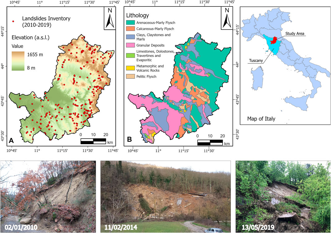
FIGURE 1. (A) elevation map of the MCF with the landslides inventory overlapped; (B) lithological map; three images of example of landslide events from the inventory used, triggered in January 2010, February 2014 and May 2019.

The MCF is located on the Tyrrhenian side of the Northern Apennine, a fold and thrust mountain system with a very complex geological structure, often prone to phenomena of instability (Rosi et al., 2018). It originated from the closure of the Ligurian Ocean, which began in the Cretaceous and lasted until the Oligo-Miocene collision between the Corso-Sardinian continental block and Adria microplate (Boccaletti et al., 1982). From the end of Miocene, due to the relaxation of the tectonic stack, the Northern Apennine was affected by deformations (Elter, 1975), still active nowadays, that produced tectonic depressions (or graben) called neo-autochthon basins, covered by fluvial and alluvial Pliocene-Quaternary deposits, separated by dorsal (or horst) with a NW–SE trend (Bonini and Sani, 2002). The bedrock is made up of flysch units, such as the arenaceous-marly flysch of the Tuscan and Umbro-Marchigian Domain, which are prevalent in the mountainous areas of North-East. The southern sectors of the area are occupied by hilly reliefs composed of eroded alluvial Pliocene-Quaternary granular and cohesive deposits (Carmignani et al., 2013) (Figure 1B).

From a climatic point of view, the MCF has a temperate climate with mild and moist winters and hot and dry summers (class “Csa” from the Köppen classification; Köppen, 1936). The mean annual precipitation varies between 600 mm/year in the south areas and in the Florence Plain and 1,200 mm/year in the mountainous areas of the north (Maracchi et al., 2005). Seasonal rainfall peaks occur in autumn and spring, particularly February and November, which are the rainiest months, whereas the minimum rainfall peak occurs in summer.

3 Materials and methods

3.1 Random Forest model

To analyse the influence of dynamic rainfall parameters on landslides triggering through machine learning model, we used a Random Forest implementation on MATLAB software code (MathWorks version R2022a, TreeBagger object of Statistics and Machine Learning Toolbox™). Random Forest model (RF) is a nonparametric and multivariate machine learning algorithm proposed by Breiman (2001) and widely used for landslides susceptibility assessment (Brenning, 2005; Catani et al., 2013; Lagomarsino et al., 2017; Canavesi et al., 2020; Luti et al., 2020; Segoni et al., 2020; Liu et al., 2021). Its popularity is due to several advantages, including the possibility of employing both numerical and categorical variables without any assumptions regarding the statistical distribution of the data. Moreover, it can automatically perform validation by building a Receiver Operating Characteristic Curve (ROC Curve) and calculating the relative Area Under the Curve (AUC). The AUC is widely used as a quantitative indicator for the predictive effectiveness of susceptibility models, ranging from 0.5 (completely random predictions) to 1.0 (perfect predictions) (Frattini et al., 2010).

RF requires the subdivision of the input database into two subsets: the training dataset, used first to train the algorithm to recognize the target event (in our case, the presence or absence of landslides), and the test dataset, used later to verify the predictive capabilities of the model. The RF model is based on the bootstrap aggregating technique, or bagging (Hastie et al., 2001): Bayesian trees are generated by splitting each node (yes/no) through observations randomly sampled from the training dataset. Observations excluded from the sampling are called Out-Of-Bag (OOB). This allows to calculate the Out-of-Bag Error (OOBE), another powerful tool of the RF model. This index, in addition to being used to find the tree with the greatest predictive capability (Luti et al., 2020), can be used to assess the relative importance of each independent variable, therefore, in our case to rank the variables according to their influence on landslides triggering (Catani et al., 2013). Essentially, for classification problems, OOBE computes the Misclassification Rate for a selected tree (t) built with the observations sampled from the training dataset, comparing the number of erroneous classifications against the total number of observations. MATLAB’s TreeBagger tool uses the following equation to calculate OOBE (Loh, 2002):

${\mathit{O}\mathit{O}\mathit{B}\mathit{E}}_{\mathit{t}}=\frac{\mathbf{1}}{{\displaystyle \sum _{\mathit{j}=\mathbf{1}}^{\mathit{n}}}{\mathit{w}}_{\mathit{j}}}{\displaystyle \sum _{\mathit{j}=\mathbf{1}}^{\mathit{n}}}{\mathit{w}}_{\mathit{j}}\left({\mathit{y}}_{\mathit{j}}\ne \overline{{\mathit{y}}_{\mathit{t}\mathit{j}}}\right)$

where $\left({\mathrm{y}}_{\mathrm{j}}\ne \overline{{\mathrm{y}}_{\mathrm{t}\mathrm{j}}}\right)$ represents the erroneous classifications, and w_j is the weight assigned to the jth observation; in our case equals to 1 because it is unknown a priori.

To estimate the importance of a variable (x), within the t-tree the value of a variable is randomly permuted, that is, an OOB observation is included, and then OOBE is computed again for the resulting tree (OOBE_tp). Subsequently, the difference (d_t) between the two errors is determined as:

${{\mathit{d}}_{\mathit{t}}\left(\mathit{x}\right)=\mathit{O}\mathit{O}\mathit{B}\mathit{E}}_{\mathit{t}\mathit{p}}-{\mathit{O}\mathit{O}\mathit{B}\mathit{E}}_{\mathit{t}}$

This measure is computed for the selected variable for each tree, then, mean ($\overline{{\mathrm{d}}_{\mathrm{x}}}$) and standard deviation (σ_x) are calculated. The estimate of the importance of the selected variable x, called OOB Permuted Predictor Importance Estimate, is:

$\mathit{O}\mathit{O}\mathit{B}\mathit{P}\mathit{e}\mathit{r}\mathit{m}\mathit{u}\mathit{t}\mathit{e}\mathit{d}\mathit{P}\mathit{r}\mathit{e}\mathit{d}\mathit{i}\mathit{c}\mathit{t}\mathit{o}\mathit{r}\mathit{I}\mathit{m}\mathit{p}\mathit{o}\mathit{r}\mathit{t}\mathit{a}\mathit{n}\mathit{c}\mathit{e}\mathit{E}\mathit{s}\mathit{t}\mathit{i}\mathit{m}\mathit{a}\mathit{t}\mathit{e}\left(\mathit{x}\right)=\frac{\overline{{\mathit{d}}_{\mathit{x}}}}{{\mathit{\sigma }}_{\mathit{x}}}$

Finally, this procedure is repeated for each independent variable, and the results are inserted into the histogram of the variables’ importance. This provides rough guidance for judging which independent variables are significant and which are not. In fact, if a variable is important in prediction, then permuting its values should affect the model error. If a variable is not important, permuting its values should have little or no effect on the model error (Breiman, 2001; Gregorutti et al., 2017).

In addition to the variables’ importance, the RF model also provides the Partial Dependence Plots (PDPs), which allow to identify the most important classes or ranges of values within each individual variable. PDPs show the relationship between each class of values from one predisposing factor and the predicted outcome of a machine learning model; therefore, they can show whether this is linear, monotonic or more complex (Friedman, 2001). The partial dependency of a binary-tree model is estimated by assigning a weight equal to 1 to the root node of a tree. Considering x_s as a value of the independent variable x, if the following node is split by x_s, it is assigned the same weight as the previous node. If a node splits by other values than x_s, the weight of each child node becomes the value of its parent node multiplied by the fraction of observations corresponding to each child node. Then, the algorithm computes the average weight for the individual tree, and for an ensemble of bagged trees the estimated partial dependence is an average of the weight over each tree (Hastie et al., 2001). PDPs are a powerful tool useful for deeply analysing the variables’ importance and therefore, in our case to prove that the statistical outcomes of the model are consistent with the physics of landslides triggering.

3.2 Dependent variable

Regarding the dependent variable, which consists of the presence or absence of landslides in a given space and in a given time, it was decided to use the database of landslides reports collected from the diary of the situation room of the civil protection of the MCF. It is an archive which collects all critical events, landslides and not, reported to the situation room. The archive contains the description of the events and the on-site interventions to restore the ordinary situation. Initially, all landslide events were selected; then, to obtain a landslides inventory suitable for the proposed analysis, they were filtered based on the reporting day, the location, and the type of landslide; and finally, they were exported in a GIS environment. The archive entries with missing information about the reporting day, location or type were automatically discarded.

The landslide date is essential to associate each landslide to the respective triggering rainfall. In the inventory generated, the reporting days of the landslide events to the situation room are indicated, which can be different from the real triggering day. The estimated temporal accuracy is 1 day; in fact, some events can be reported later than the real instant of triggering, in particular for those events occurred in remote locations and during the night, without causing critical damage and therefore reported only several hours later.

All the landslides contained into the inventory were georeferenced according to the descriptions provided by the diary. Accurate information is often available, such as the GPS coordinates of a landslide point; however, in some cases, the information is incomplete or absent, making georeferencing impossible. In these cases, the landslides were discarded. Specifically, the landslides were georeferenced as point geometry using GPS coordinates or through meticulous research of the trigger points using Google Maps and all the information contained in the diary, and lastly, using the road references reported in the diary, usually containing the exact milestone. Therefore, the estimated error is maximum 1 km for the events georeferenced through the road references without the milestone information but knowing only the road kilometres.

Another key feature is the correct description of the type of landslide. It is necessary to use for the proposed analysis only those events whose triggering is due to rainfall only, as shallow landslides and debris or mudflows. Other types of landslides for which rainfall is not the main triggering factor (for example, rockfalls or anthropic-induced landslides) have been discarded. In the analysed period, there were no landslide linked with main earthquake events, so the presence of earthquake-triggered landslides can be excluded.

Therefore, from the diary of the situation room, a total of 410 landslides were extracted, mainly shallow landslides and small debris or mudflows, for the period from 2010 to 2019; with an estimated spatial and temporal resolution of 1 km and 1 day (Figure 1A) respectively.

3.3 Independent variables

As independent variables, expressing the landslides predisposing factors, it was decided to use the parameters listed below.

- Cumulative rainfall (CR_x [mm]): cumulative rainfall computed at various time steps (with x ranging from 1 to 30 days). This represents the first dynamic parameter used in this study to test the capability of the RF algorithm in recognizing the importance of rainfall in landslide triggering. In fact, landslides can be divided into two main types: shallow landslides and deep-seated landslides. There is a general agreement in literature that shallow landslides are primarily triggered by short-term and intense rainfall, which causes the rapid infiltration of abundant water into the soil and determines the increase in water pressure. The activation of deep-seated landslides, on the other hand, is influenced by long-term rainfalls, even with a lower intensity, as they require longer infiltration times (Martelloni et al., 2012; Tehrani et al., 2022). The cumulative rainfall allows to consider both short-term but intense rainfall (for instance, the cumulative rainfall between 1–3 days) and long-term but less intense rainfall (for instance, the monthly cumulative rainfall), and therefore both types of landslides.

 Consequently, the cumulative rainfall from 1 to 30 days from 2010 to 2019 was calculated using the meteorological radar data provided by the Italian Civil Protection Department (Figure 2). Meteorological radars are ground-based remote sensing systems that operate in the microwave band and measure the electromagnetic pulse reflected by water drops within a 200 km radius to estimate the rainfall intensity. In fact, the measured reflectivity value is converted to rainfall intensity using the Marshall-Palmer equation:

FIGURE 2

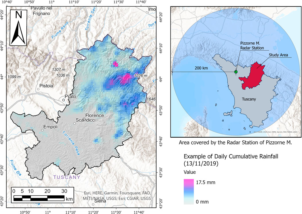
FIGURE 2. Example of radar daily cumulative rainfall (for 13/11/2019) from meteorological radar data.

$\mathit{R}={\mathit{\alpha }\mathit{Z}}^{\mathit{\beta }}$

 where R represents the rainfall intensity (mm/h), Z is the reflectivity calculated on the radar pulse duration (mm⁶/m³ or decibel) and α and β are empirical coefficients that vary according to the type of precipitation measured (whether stratiform or convective), and regarding the state of the water composing it (liquid, snow, or hail) (Marshall and Palmer, 1948; Petracca et al., 2018). The Italian Civil Protection Department manages a total of 24 radars distributed throughout the national territory, and the nearest meteorological radar station to the MCF is on the Pizzorne Mount, in the Lucca province, which covers the entire Tuscany region. Radar data were used instead of rain gauges because they provide spatialized data, making the association between landslides and related rainfall more accurate. The data used is called Surface Rainfall Intensity (SRI), which expresses the amount of water falling on the ground surface for the duration of the radar pulse. The database contains data at 5 min temporal resolution, from 2010 to 2019, in BUFR format (Binary universal Form for the Representation of meteorological data). The data were converted into ASCII format and then summarized to obtain the cumulative rainfall from 1 to 30 days from 2010 to 2019. Unfortunately, the radar database contains some gaps; therefore, only 315 out of 410 landslides can be associated with 30 day antecedent rainfall and can be fully used for the proposed analysis.

 The use of cumulative rainfall at various time steps as independent variables allows to consider both the rainfall occurred on the reporting day and those that occurred in the previous days; therefore, the temporal error contained into the landslide database can be considered negligible. In addition, the spatial resolution of the radar data is 1 km, which is comparable to the maximum spatial error of the used landslides.

- The month of observation of the events (landslide or non-landslide events) (Month [-]): this second dynamic parameter, inserted as a categorical type (from 1 to 12), was used to observe if the RF model can conveniently use the information on rainfall seasonality to improve predictions. The seasonal variability is considered one of the most influential factors in triggering landslides (Gariano and Guzzetti, 2016), in fact, less intense and short-term rainfall can trigger landslides if it occurs during the wet season rather than in the dry season, because it will occur into an already partially saturated soil with an already high water pressure (Segoni et al., 2018b; Rosi et al., 2021).

- Landslide Susceptibility Index (LSI [-]) (Figure 3A): it represents the landslide susceptibility map with a spatial resolution of 100 m² developed for the study area by means of the RF model application with the base independent variables, which does not include the newly proposed dynamic parameters but only a set of static parameters commonly used in literature: elevation, slope, aspect, total curvature, profile curvature, planar curvature, lithology, and land use (Reichenbach et al., 2018; Segoni et al., 2021). It was decided to use a base LSI to observe more clearly how the RF model considers dynamic rainfall parameters respect to the main static geological characteristics for the spatio-temporal landslides prediction. In addition, the direct use of landslide susceptibility as input data, instead of every single geomorphological parameter, reduces computational time. Because LSI has only a spatial meaning, while the dynamic application it will add the temporal information, inserting LSI as input variable does not intentionally help the dynamic model to make predictions, since the landslides data are treated in a completely different way in the two cases. For this reason it will be necessary to perform in a further step the training and testing phases also for the dynamic model. To create the LSI, as dependent variable, the events contained in the abovementioned inventory were integrated with other 69 events for the period 2000–2009, chosen among those with higher spatial accuracy from Rosi et al. (2015); for a total of 479 landslides. Each landslide is geolocated as punctual geometry, and this might be a problem for the susceptibility assessment, because the characteristics of the area around these points are considered peculiar of stable area, whereas they could belong to the landslides body with a high probability; this misclassification can lead to unreliable results. For this reason, it was decided to recreate the unstable area affected by landslides through an alternative elaboration in GIS environment and described in Figure 3B: using the Watershed tool in ArcGIS PRO, the drainage areas upslope each landslide point was defined, thus defining a portion of the slope upstream of the landslide point in which the water flows into it. Some of these polygons occupied large areas, so they were clipped with a 100 m buffer from the landslide point. The resulting polygon can be considered a good approximation of the area subject to instability, much more realistic than the simple buffer, and can be proposed in cases such as this, where the polygonal landslides database is not available.The model for LSI was applied using 500 trees, in order to obtain a more stable OOBE. Initially, a random parameter with values between 0 and 1 was inserted among independent variables in order to observe the model response. Then, once it was verified the ability of the model to recognize this variable as irrelevant in landslides triggering, it was discarded. The database contains 479 landslide polygons, which occupy a total of 30′167 pixels with a 10 m resolution. The same number of pixels was selected to identify the non-landslide points. The database was divided into two portions: 70% for the training phase and 30% for the test phase. Subsequently, the model was reapplied to all pixels in the study area (35′128′678 pixels) for a further validation. The map obtained was then resampled at 100 m resolution to make it more homogeneous. This spatial resolution is adequate to connect each landslide point with the correct susceptibility value, in order to conduct the analyses proposed in this study. The map obtained has an AUC value of 0.86, and the Efficiency, which is the ratio between the number of correct predictions (sum between True Positive or TP and True Negative or TN) versus the number of total predictions (sum between the abovementioned correct predictions and wrong prediction, the False Positive or FP and False Negative or FN), returns a value equal to 0.80, demonstrating an accurate spatial prediction of landslides. The OOB variable’s importance method classifies as the most significant variables, in order: elevation, lithology, slope, and land use. The use of LSI as an input to the dynamic model does not lead the latter to overfitting problems, because it does not represent a faithful map of the landslide’s perimeter. This is demonstrated by the use of a larger landslide inventory to develop LSI than that employed in the subsequent dynamic modelling, and by the obtained value of AUC, far from 1, which would instead indicate a prediction perfectly faithful to the landslide inventory.

- Random variable (Random [-]): to monitor the effectiveness of the variables used, was also included in the analysis a random variable, with values between 0 and 1. This parameter is used as a control to identify (and discard) any independent variable with a predictive power similar to the one assigned to the Random variable and evidently not linked with landslide triggering.

FIGURE 3

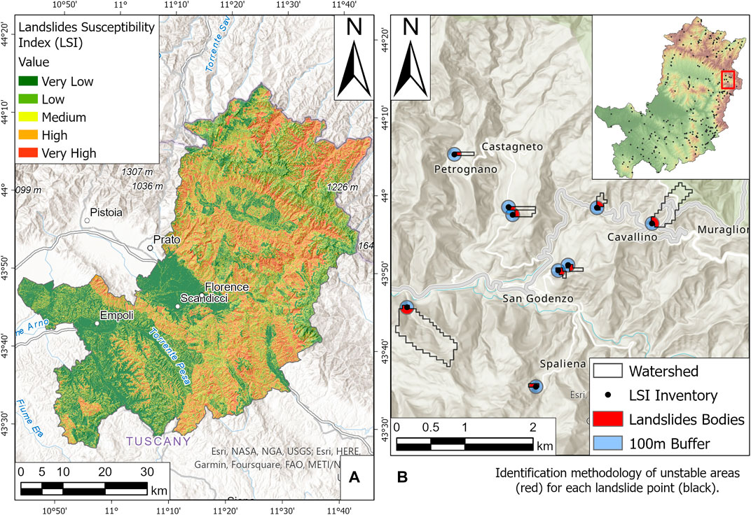
FIGURE 3. (A) map of Landslides Susceptibility Index (LSI); (B) magnification depicting the proposed method to recreate the landslides bodies.

4 Methods

The application of the RF model requires a pre-processing of the input data. The independent variables are placed in overlapping layers, then sampled for each landslide point. In the same way we proceed with nonlandslide points, which are chosen in equal number to landslide points to balance the database, in a random way. Finally, the samples are inserted into a matrix that represents the input of the RF model. For the realization of a landslide susceptibility map with this method both landslide events and non-landslide events vary only in space and not in time, so it is not possible to insert dynamic variables as input data. For this reason, the resulting susceptibility map represents the spatial probability of occurrence of landslides projected into the future valid as long as the input variables remain constant over time (Fell et al., 2008). In our research, several tests have been carried out to account for both spatial and temporal variability of landslide and non-landslide events. The goal is not to set up a landslide probability map, but to observe which rainfall variables had a statistically significant influence on the time and location where landslides occurred, to verify the applicability of a forecasting model based on the proposed dynamic approach.

4.1 Data pre-processing

Six different methods of pre-processing the data were analysed, listed below and summarized in Table 1, based on the identification of non-landslide events in comparison with the reporting day and the location of the landslide. The first three tests are developed to use a balanced database, so in our case, with 315 non-landslide events and 315 landslide events.

- first test: the non-landslide events were selected in the same pixels compared to the landslide events, but on different days selected randomly;

- second test: the non-landslide events were selected on the same day compared to the landslide events, but in different pixels selected randomly;

- third test: the non-landslide events were selected at randomly generated pixels and days, both different from the landslide events.

TABLE 1

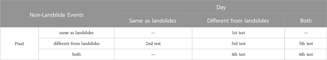
TABLE 1. Summary table of the six tests used in the proposed methodology. Each non-landslide event was selected by comparison with the days and the pixels of the landslide events.

The other three tests were performed by a mixed criteria, merging the aforementioned datasets with different combinations, accounting for all possible approaches to select non-landslide events: both same and different pixels and/or both same and different days. For the previous three tests, each landslide event was balanced by a non-landslide event (1:1 ratio), but in the mixed criteria cases, we used an unbalanced database (1:2 ratio between landslides and non-landslide events) to better represent all possible definitions of non-landslide events in the training dataset.

- fourth test: 315 non-landslide events were sampled in the same pixels of the landslides and other 315 in different pixels, in both cases on different days, compared to landslide events;

- fifth test: 315 non-landslide events were selected on the same days of the landslides and other 315 on different days, in both cases in different pixels, compared to landslide events;

- sixth test: test generated by merging the first two tests, but with new non-landslide events chosen randomly; so, 315 non-landslide events were chosen in the same pixels but on different days of the landslides and another 315 were chosen on the same days but in different pixels, compared to the landslides.

4.2 Model configuration

A crucial step in the model setting is the choice of the database splitting method for training and test phases. It was chosen to analyse four different model configurations, listed below and summarized in Table 2

- first configuration: for the first run of the model, the analysis was performed using all the independent variables listed above (cfr. Section 3.3). The database of observations (landslide plus non-landslide events) was divided into two datasets: one for the model training (containing 70% of the observations) and one for the model testing (containing the remaining 30%). For the first three tests, with a balanced database (same number of landslide and non-landslide events in each dataset), both the training and testing datasets contained 50% landslide events and 50% non-landslide events. Instead, for the other three tests with an unbalanced database (number of non-landslide events double than the number of landslide events), also the training and testing subsamples are unbalanced, with the same relationship 1:2, therefore with 33.3% of landslide events and 66,7% for non-landslide events.

- second configuration: another run with all the independent variables as input data was carried out, but with a highly unbalanced database with a relationship of 1:10 for every test, so containing all the 315 landslide events and 3,150 (ten times more) non-landslide events, and also the training and test subsample are unbalanced with the same relationship, so with 9% of landslide events and 91% of non-landslide events. The aim of using this strongly unbalanced databases is to verify if, with a higher number of non-landslide events than landslide events, the results in terms of variables’ importance do not vary and if the model is still able to recognize the influence of rainfall on the spatial and temporal occurrence of landslides. It is important to test the capability of the model with unbalanced datasets because they are more representative of the real population of events, where pixels and days without landslide are much more numerous than those with landslide.

- third configuration: the same as the first configuration (i.e.,: for the first three test was used a balanced database 1:1 and for the other three tests was used an unbalanced database 1:2, between landslide and non-landslide events). The main difference lies in the fact that for this configuration, the analysis was carried out only with the most important short-term cumulative rainfall found by applying the previous configurations, some symbolic long-term cumulative rainfall (in particular, the ones at 7, 14, 21, and 30 days), the Month and the LSI variables.

- fourth configuration: the same as the second configuration (i.e.,: for each test was used an unbalanced database 1:10, between landslide and non-landslide events). In addition, in this case, fewer independent variables are used as inputs, as well as the third configuration.

TABLE 2

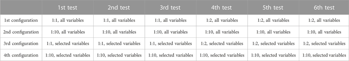
TABLE 2. Summary table of the four configurations used in the proposed methodology, summarizing the ratio between training and test samples and the number of independent variables used as input for the RF application.

For each configuration, the model was run 7 times, to observe whether the results vary with the random selection of training and test database and to obtain the confidence interval; for a total amount of 168 model applications. Finally, all runs were carried out by building 2000 trees, until a more stable OOBE is obtained.

5 Results

In this chapter, the results obtained are presented in two consecutive steps. First, we compared the variables’ importance by the histograms of OOB Permuted Predictor Importance Estimate, to verify the consistency of the model with the mechanism of triggering of the landslides analysed. Second, we use the PDPs to compare not only the variables amongst themselves, but also to compare each class or value of each variable, to understand more deeply if the RF algorithm follows a physically correct scheme to link dependent and independent variables.

5.1 OOB Permuted Predictor Importance Estimates

The variables’ importance for each test and configuration is shown from Figures 4–7. The histograms were obtained by averaging the outcomes of the 7 model runs, and the error bars show the maximum and the minimum values of importance found as confidence intervals.

FIGURE 4

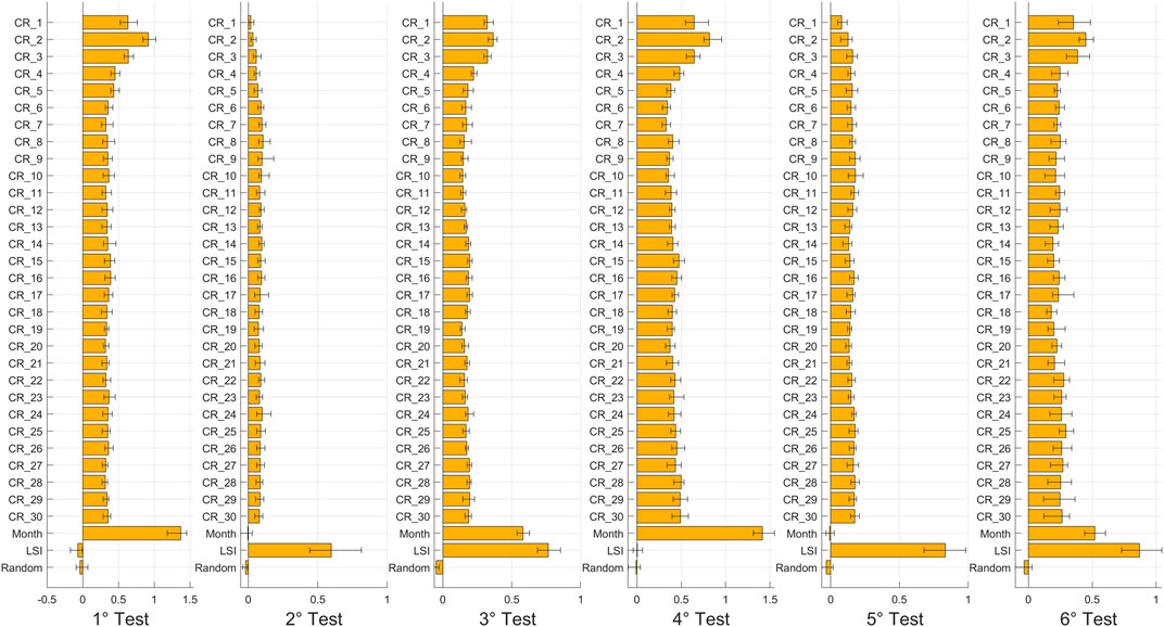
FIGURE 4. Histograms of OOB Permuted Predictions Importance Estimates for each test for the first configuration.

FIGURE 5

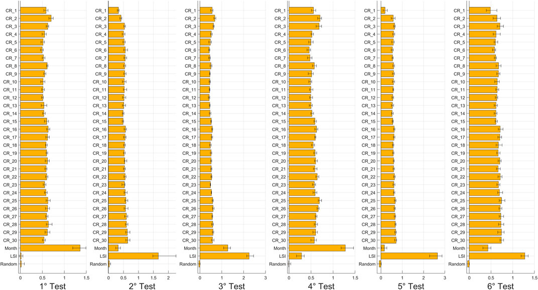
FIGURE 5. Histograms of OOB Permuted Predictions Importance Estimates for the second configuration.

FIGURE 6

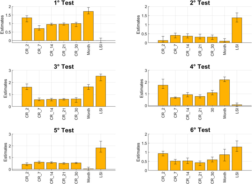
FIGURE 6. Histograms of OOB Permuted Predictions Importance Estimates for the third configuration.

FIGURE 7

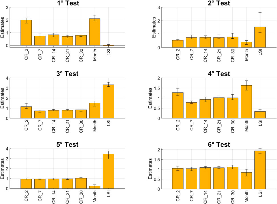
FIGURE 7. Histograms of OOB Permuted Predictions Importance Estimates for the fourth configuration.

First, for each figure, the Random variable shows low or negligible importance. Negative OOB values identify pejorative input variables that increase the error of the prediction: the model recognizes the irrelevance of the Random parameter, as expected, and allows recognizing, in a few configurations, some variables that play a role less meaningful than a random number. Thus, the Random variable and all parameters with similar importance were removed for the analysis of third and fourth configurations.

For the first configuration, Figure 4 shows that the short-term rainfall (i.e., the cumulative rainfall at 1, 2, and 3 days) are the most important rainfall variables for the first and fourth tests, which have in common the choice of non-landslide events on different days from the landslides. In addition, for them, the Month variable is the most important, and the LSI is the least important. This result is not surprising and is explained by the model configuration: if non-landslide events are chosen in the same pixel but on different days with respect to the landslide events, then the difference between stable and non-stable instances depends only on the rainfall characteristics at the time of the sample. In fact, the susceptibility index cannot be effectively used to discriminate between stable and unstable instances in this case because all samples were taken in unstable zones, but at different times, and LSI cannot take this dynamic factor into account. Conversely, for the second and fifth tests, which have in common the choice of non-landslide events in different pixels from the landslide events, rainfall has a low value of importance, the Month variable is the least important, and the LSI is the most relevant. Instead, in these cases, the difference between stable and non-stable instances depends mainly on the susceptibility value in the location of the sample, and secondly on the spatial variability of rainfall. The seasonal variability, expressed by the Month variable, cannot be used to explain this spatial variability. Indeed, for the third and sixth tests, which have in common the use of both different pixels and days to identify non-landslide events against landslide events, the results are a merge of those of previous tests. In both cases the short-term rainfalls are the most important rainfall, and the Month variable has a high importance, as in the first and fourth tests; but also the LSI has a very high importance, as in the second and fifth tests.

These results are also confirmed for the second configuration, shown in Figure 5, but here the differences of importance are fading due to the effects of using a highly unbalanced database. The most important short-term rainfall is the 2-day cumulative rainfall, while for longer rainfall durations, the cumulative rainfalls in a weekly step (namely, at 7, 14, 21, and 30 days) were selected as the most representative parameters. This is because, for long periods, the values of importance are very similar, and it is not possible to identify which of these cumulative rainfalls is the most representative. These data, along with the month and the LSI variables, were used to carry out the configurations 3 and 4. As mentioned above, the Random variable, as well as the other less relevant cumulative rainfalls, were removed from the analysis.

These outcomes are confirmed in the third (Figure 6) and the fourth (Figure 7) configurations, in which it’s observed an increased difference between long-term rainfalls, the least important variables, and the short-term rainfalls, the Month and the LSI variables, which are the most important, even with the use of a highly unbalanced database.

5.2 Partial Dependence Plots

Due to space constrains, from Figures 8–10 are depicted the PDPs only for the first, second, and third tests and the first configuration, that is, of the most representative cases. They showed the results for the most representative variables, namely, the cumulative rainfall at 1, 2, 3, 7, 14, 21, and 30 days, the Month, the LSI and the Random variables, to observe the general relationships among them and the model output. The graphs contain the curves obtained for each of the 7 models run to account for the confidence interval.

FIGURE 8

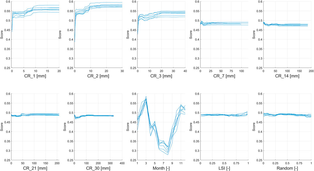
FIGURE 8. PDP for the first test and the first configuration.

FIGURE 9

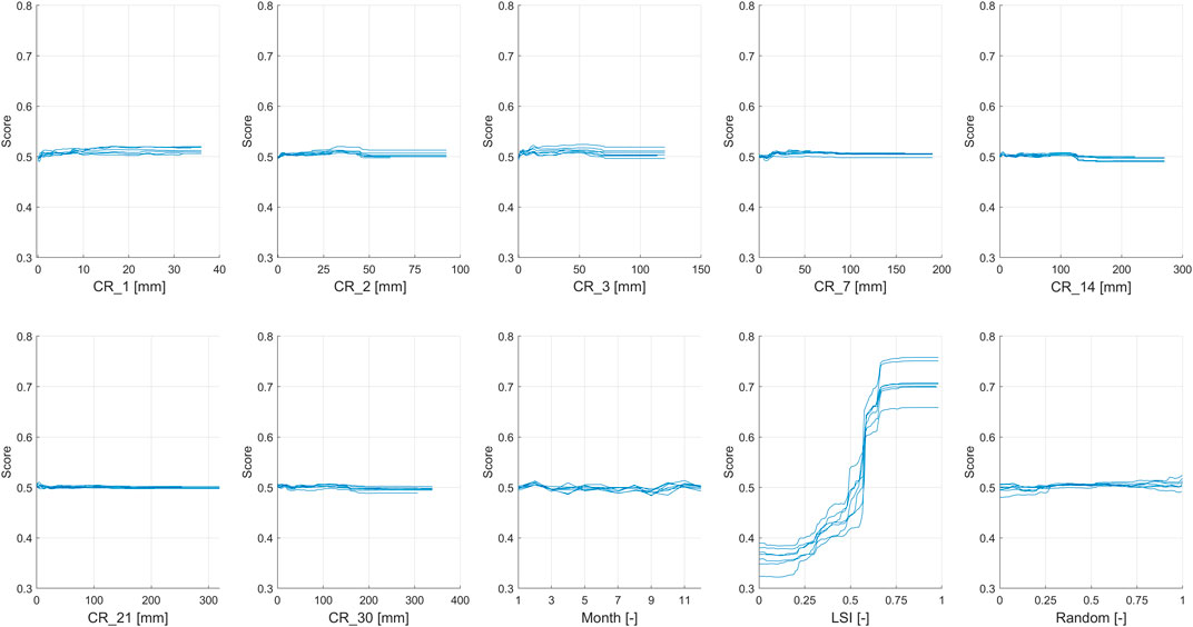
FIGURE 9. PDP for the second test and the first configuration.

FIGURE 10

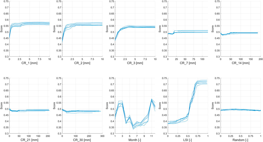
FIGURE 10. PDP for the third test and the first configuration.

The PDP of the first test (Figure 8), which identifies the non-landslide events in the same pixels but on different days from the landslides, shows a convex shape for the short-term rainfalls, indicating a lower importance for the less intense rainfalls and a greater importance for the most intense rainfalls, as expected, until a peak is reached, greater for the 2 days duration, beyond which the importance assumes a constant value. For the cumulative rainfall at 7 days, it is still possible to recognize the convex trend, even if with a lower peak; then, for the other cumulative rainfall values the PDP graphic is almost flat, demonstrating that longer durations do not have any clear relationship with the model outcome. The Month variable presents a multivariate behavior, with the main positive peak in February, March (end of winter and beginning of spring) and November (autumn) and the lowest peak during the summer (June, July, and August). The PDP of LSI is flat, confirming the results found in the variables’ importance analysis for the same test, in which LSI has no importance in this case.

For the second test, which identifies the non-landslide events on the same days but on different pixels from the landslides, the PDPs of each cumulative rainfall are flat, as shown in Figure 9, indicating the absence of a relationship with the model outcome. Even for the Month variable, it is not possible to recognize a clear relationship. For LSI the curve starts from a low and flat importance that remains constant until a rapid increase among LSI value equal to 0.5, reaching a peak at about 0.75 and again continue with a constant and flat trend, showing a strong relationship with the model output.

The PDP of the third test (Figure 10), which identifies the non-landslide events both on different days and different pixels from the landslides, seems to be a combination of the previous two tests. The short-term cumulative rainfalls and the Month variables show a strong relationship, for the first ones with a convex curve, with the intense rainfall events as the most important against the low intense ones, and the second one with positive peaks during the months of February, March, and November, and a negative peak during the summer, similar to the first test. While the LSI shows a trend starting from a low and flat importance under the LSI value of 0.5; then shows a rapid increase until a peak at about 0.75, as well as the second test. The long-term rainfall and the Random variables are flat, showing no relationship with the model outcome, as well as both first and second tests.

Figure 11 shows the PDPs obtained for variable CR_2, for the third test, for all configurations. Between first and third configurations, no significant differences can be observed: the peak of importance of CR_2 is reached for values of rain around 2.5 mm. Instead, moving from balanced to unbalanced dataset, a shift of the peak to higher values of rain is observed: for second and fourth configurations, it reaches values of about 30 mm.

FIGURE 11

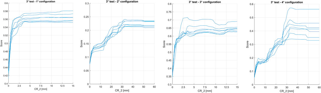
FIGURE 11. PDPs obtained for variable CR_2, for the third test, for all configurations.

It was decided to further investigate how the peak of importance of PDPs of the CR_2 variable varies by increasing the degree of imbalance. Imbalanced datasets were generated by considering a number of non-landslide events equal to 3, 5, 7, 20, 50 and 100 times the landslide events. The configuration with only the selected cumulative rainfalls was tested. The results are shown in Figure 12 (the symbology x3, x5, x7, x10, x20, x50 and x100 indicate the degree of imbalance of the database). It was observed that as the degree of imbalance increases, there is a progressive shift of the peak of importance of CR_2 to higher values of rain: from a peak of approximately 2.5 mm for the balanced database, a rapid increase is observed, up to about 20 mm for the unbalanced database x5, and up to approximately 30 mm for the unbalanced database x7. After that, as the degree of imbalance increases, the peak remains quite stable, at about 30–35 mm. By increasing the number of observations available, a more accurate frequency distribution of rainfall is obtained, at which the model is readapted, finding a new logical scheme used to discriminate ordinary events from those that trigger landslides.

FIGURE 12

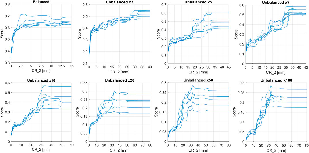
FIGURE 12. PDPs of the CR_2 variable obtained by applying the third test, with only the selected cumulative rainfalls, and using a balanced database or different degree of imbalance (x3, x5, x7, x10, x20, x50 and x100).

6 Discussions

Regarding the results obtained from the histograms of variables’ importance, they show a clear influence of short-term cumulative rainfall and the Month variable for first and fourth tests, while for second and fifth tests LSI is the most important one. These differences are lead by the method used for the identification of non-landslide events; in fact, the common feature between first and fourth tests is the choice of non-landslide events on different days from the landslides; therefore, in these cases, the analysis is focused on the temporal prediction, for this reason the dynamic parameters are the most important and LSI has no influence. The opposite situation can be verified in the second and fifth tests, that have in common the choice of non-landslide events in different pixels from the landslide events. In these cases, the analysis is focused on the spatial prediction, so the static parameter, the LSI, is the most important one, and the dynamic ones are the least important. The third and sixth tests account both different pixels and days from landslide events to identify the non-landslide events, even if in different proportions, so these analyses are focused both for spatial and temporal forecasting, and in fact, both dynamic and static parameters show an influence on the model outcome; and this is a more realistic situation in respect to the other tests.

The most important short-term rainfall is the cumulative rainfall of 2 days. This means that, generally, to initiate a landslide, a certain time interval after a rainfall event is needed to build the necessary pore water pressure, which is obtained after more than 24 h. This result can also be influenced by the dating accuracy of some landslides, which can be reported the day after the triggering. LSI is the most important parameter for the majority of the tests, proving the high influence of the geological and geomorphological characteristics of the study area on the assessment of the exact location where landslides may be triggered.

For the third test, the PDPs show a convex trend for short-term rainfalls, this means that the less intense rainfalls are less important than the more intense rainfall, as expected. The long-term rainfalls seem not to have any relationship with the model outcome; this is in line with what was expected, because this study was carried out for a landslide inventory composed of shallow landslide, mainly affected by short-term but intense rainfalls. With regard to the Month variable, the PDPs show a multivariate trend, with positive peaks during the wet seasons and negative peaks during the dry seasons. This result is in line with what was expected, because during the wet season, even less intense rainfall is sufficient to trigger landslides, due to the presence of an already partially saturated soil, and the opposite occurs during the dry season, in which a higher rainfall amount is necessary to trigger landslides, because the soil is completely or almost dry. The use of the Month variable can contribute to enhancing the results in a logical way, showing that this variable is used by the machine learning algorithm as an empirical proxy for the humidity of the soil. As expected, the PDPs of the LSI variable show an ascending importance with the increase of the susceptibility value.

It was also verified that the peak of importance of the PDPs of the variable CR_2 by increasing the degree of imbalance of the database progressively moves towards higher values of rain. It goes from a value of 2.5 mm for the balanced database to 30 mm for the unbalanced database x7; the peak then remained stable until the unbalanced database x100. This behavior can be interpreted considering that, by increasing the number of observations, the model recognizes the 2.5 mm rains as actually more frequent than those observed with a balanced database. In response, the model shifts the peak of importance towards higher values of rain to better discriminate the rain that causes the triggering of landslides, generally more intense, from the ordinary ones, less intense. The use of an unbalanced database is also consistent with the real frequency distribution of landslide and non-landslide events, the latter more frequent than the former; however, considering an incomplete landslides inventory, it could be potentially possible to identify not reported landslides as non-landslide events. These erroneous classifications could lead to a greater uncertainty of the results, so the imbalance should be carefully evaluated. For instance, this test shows that the x7 imbalance seems to be the optimal one to be used in similar analyses: an increase in the unbalanced proportion did not produce significant modification.

These results are in line with the actual knowledge of the physical mechanism of the triggering of shallow landslides and debris or mud flows, which are mainly influenced by short and intense rainfalls, the seasonality that reflects the degree of saturation of the soil, and the predisposition to landslide of the study area. The tests that seem to have the highest capability of representing the real situation are the third and sixth tests, for each configuration: they account for non-landslide events that vary over both space and time and show a high importance of both dynamic (short-term rainfall and Month) and static (LSI) variables. Using an unbalanced dataset can also help to better represent the real situation, because landslide events are much less numerous than non-landslide ones and increasing the observations allows to consider a more representative frequency distribution of rainfall. Therefore, the RF model applied through the proposed methodology shows encouraging results, representing a promising basis for understanding how to sample non-landslide events over space and time for the population of training and test datasets, identifying the most important variables and to verify the applicability of machine learning models for landslides probability assessment.

To verify again the results obtained and to better understand which is the test and the configuration with the highest predictive power, looking for a future application of the model for landslides forecasting activities, a performance analysis is mandatory. The AUC value is calculated for each test and configuration; for each of the 7 model runs, then averaged. The results are shown in Figure 13. We observed that the highest AUC value is obtained for the third test, the one with non-landslide events chosen both in different pixel and days from the landslides, and for the third and fourth configurations, those with a lower number of input variables, but only the most representative ones, namely, with AUC values equal to 0.90 and 0.91 respectively. The third test results the better once again, confirming the results described above.

FIGURE 13

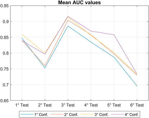
FIGURE 13. Mean AUC value for each test and configuration.

For the performance analysis, we calculated the number of TP, FP, TN and FN for each test and configuration, for each model run, then averaged. They are used to calculate several statistical indices that are commonly used for model prediction performance evaluations (Calvello and Piciullo, 2015; Piciullo et al., 2020; Bulzinetti et al., 2021). The extremely high number of TN for the tests and configurations with an unbalanced database could lead to unreliable results of performance analysis. To avoid this issue, statistical indicators that do not account for the number of TN have been mainly used, with the exception of the Efficiency, where the TN number is used both at numerator and denominator. In Table 3 all the used performance indicators are listed along with their equations, and in Figure 14 the graphs obtained for each test and configuration are shown.

TABLE 3

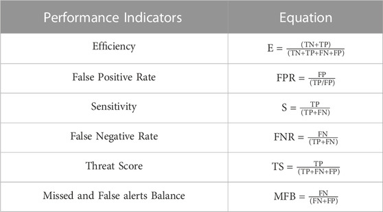
TABLE 3. List of performance indicators used in the analysis and their equations.

FIGURE 14

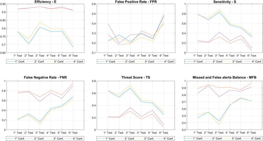
FIGURE 14. Trend of the various performance indicators analysed based on each test and combination.

As regard the tests, the highest values of E (Efficiency), S (Sensitivity) and TS (Threat Score) have been observed in the third test, due to the high number of TP obtained for this test. Instead, for FNR (False Negative Rate) and MFB (Missed and False alerts Balance) the third test shows the lowest values, which indicate a low number of FN. The lowest values of FPR (False Positive Rate) indicates the lowest number of FP and is reported for the second and third tests.

As regard the configurations, E is high for the third and fourth configurations, because of the high values of TN associated with the unbalanced database. The first and second configurations have the highest values for S and TR, indicating a high number of TP. They have the lowest value for FNR and MFB, indicating that they have the lowest number of FN. For FPR the second configuration presents the lowest value, but only for the second and sixth tests, with a very low difference with the third configuration, who are on the same level for the third test.

Observing the trend of TP, FN, and FP with the increase in the degree of imbalance (Figure 15), it is possible to notice, beyond a gradual decrease in TP and a consequent increase in FN, also a decrease in FP, which is already halved with an unbalanced database x3, which can represent a positive result with the prospect of using such model in an early warning system. Therefore, the imbalance of the database could be a factor on which it worth to focus for the calibration of the model, in order to obtain more realistic landslide probability maps, with a reliable predictive capability.

FIGURE 15

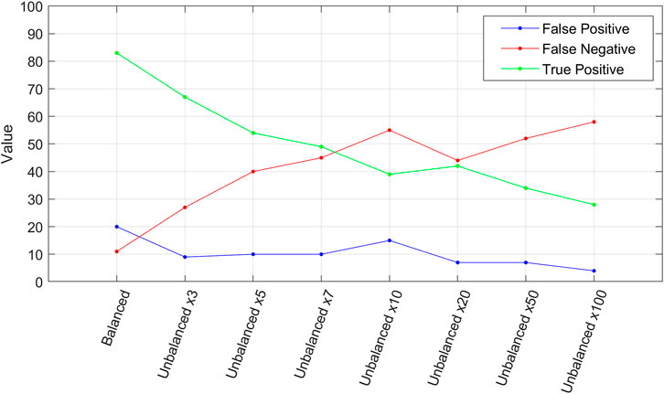
FIGURE 15. Variation of the number of TP, FP and FN varying the degree of imbalance of the database.

In a previous research (Collini et al., 2022), the SIGMA model (Martelloni et al., 2012), a rainfall thresholds-based landslides forecasting model, was applied to the same study area using the same source to collect the landslide inventory. A comparison of the evaluation metrics of the SIGMA model and of the method proposed in this study was carried out, to further validate the results obtained. The values of AUC and S obtained with the proposed method are greater than the ones obtained by applying the SIGMA model (0.91 and 0.83 against 0.53 and 0.06, respectively); while the value of E is slightly lower (0.84 against 0.99). This shows that the proposed approach can compete with the traditional statistical methods. Further comparisons with different models will be essential in order to move toward a LEWS based on the proposed approach. Summing up, this analysis of the model’s performance indicates that the third test, which defines non-landslide events both in different pixels and days from landslide, leads the machine learning model to get the highest predictive power; especially when a configuration that balances the possible occurrences of landslide and non-landslides in the input datasets is used and when only a selected ensemble of significant explanatory variables is selected. This is in line with the results obtained for the variables’ importance and PDPs analysis, which highlighted the third test as the most suitable to represent the real situation and to account for both a spatial and a temporal prediction at the same time.

7 Conclusion

Machine learning models are widely used to devise susceptibility maps, representing the spatial probability of occurrence of landslides, but to date have not been established as a consistent approach to obtain spatiotemporal prediction of landslides over wide areas. We propose a methodology for the application of a machine learning model including dynamic variables, such as cumulative rainfalls at various time steps, to observe the model behaviour and verify the possibility of a future application of this methodology not only for spatial but also temporal prediction purposes.

We used the RF algorithm, in an implementation that allows to calculate OOBE and PDPs, two statistical indexes used in this study to verify which model configuration and which variables are consistent with the physical mechanism of the triggering of the modelled landslides.

The study area is the MCF, located in Central Italy, chosen for the availability of a comprehensive landslides inventory reporting more than 300 landslides in the last decade, mainly rainfall-induced shallow landslides.

The first dynamic independent variables are the cumulative rainfall at various time steps, from 1 to 30 days, to consider both critical and antecedent rainfalls. The second dynamic variable is the Month, which is used to consider the seasonality of the rains and therefore the soil saturation conditions. As a static variable, a susceptibility map, named LSI, was inserted directly as an input variable to compare the dynamic rainfall variables with the static predisposition to landslide of the study area.

The proposed methodology is based on the evaluation of several tests conducted to account both spatial and temporal variability of landslide and non-landslide instances. Namely, we identified 6 possible tests based on different combinations for the individuation of non-landslide events. In addition, each test was applied for 4 different model configurations, based on the number of non-landslide events and the number of variables used. The results were analysed using the histograms of variables’ importance, the PDPs, and some performance indicators to verify if are consistent with the mechanism of triggering of the landslides analysed, and to identify which test and configuration show the highest predictive power, in the perspective of a future application for spatio-temporal forecasting of landslides.

We conclude that the results are consistent with our knowledge of the physics of the slope failure mechanism for shallow landslides. In fact, the most important rainfalls are the short-term ones, with an increase in importance for the more intense rainfall, the rainfall seasonality results extremely important, particularly during the wet months in which the landslides probability is expected to increase and LSI is also extremely important, confirming the key role of a well-developed landslide susceptibility analysis. The third test, characterized by the choice of non-landslide events both in different pixels and days from the landslide events, was identified as the method that led the model to obtain the highest predictive capabilities, and it was observed that the degree imbalance of the database plays a key role in the model calibration, as it allows to consider a more realistic characterization of the events. Therefore, the RF model employed through the proposed methodology shows encouraging results and represents a promising preliminary research for what is the final goal: the landslide probability mapping through machine learning approach. The original methodology proposed in this manuscript represents a general approach that can be applied elsewhere to accomplish spatial and temporal prediction of landslides at the same time; however, the specific results obtained are highly site-specific and for other applications it is advisable to calibrate the method from the start to identify a specific optimal parameters’ configuration, especially if other landslide typologies and other dynamic parameters are considered.

Data availability statement

The raw data supporting the conclusion of this article will be made available by the authors upon request.

Author contributions

NN has conceived the work, performed the analysis, contributed to the interpretation of the results and wrote the manuscript. AR has conceived the work, contributed to the interpretation of the results and to write the manuscript. SS has contributed to the interpretation of the results and to write the manuscript. RF has supervised the work.

Funding

This work was funded by “Dipartimento della Protezione Civile-Presidenza del Consiglio dei Ministri” (Presidency of the Council of Ministers-Department of Civil Protection); this publication, however, does not reflect the position and social policies of the Department.

Acknowledgments

We gratefully thank the civil protection of the Metropolitan City of Florence, for making available the landslide reports collected to obtain the inventory used in this study.

Conflict of interest

The authors declare that the research was conducted in the absence of any commercial or financial relationships that could be construed as a potential conflict of interest.

Publisher’s note

All claims expressed in this article are solely those of the authors and do not necessarily represent those of their affiliated organizations, or those of the publisher, the editors and the reviewers. Any product that may be evaluated in this article, or claim that may be made by its manufacturer, is not guaranteed or endorsed by the publisher.

References

Abraham, M. T., Satyam, N., Rosi, A., Pradhan, B., and Segoni, S. (2020). The Selection of rain gauges and rainfall parameters in estimating intensity-duration thresholds for landslide occurrence: Case study from Wayanad (India). Water (Switzerland) 12, 1000. doi:10.3390/W12041000

CrossRef Full Text | Google Scholar

Bianchi, C., and Salvati, P. (2022). Rapporto Periodico sul Rischio posto alla Popolazione italiana da Frane e Inondazioni. Istituto di Ricerca per la Protezione Idrogeologica (IRPI). Consiglio Nazionale delle Ricerche (CNR). Available at: polaris.irpi.cnr.it (Accessed July 20, 2022).

Google Scholar

Bishop, C. M. (2006). Pattern recognition and machine learning, 4. New York: Springer. No. 4.

Google Scholar

Boccaletti, M., Decandia, F. A., Gasperi, G., Gelmini, R., Lazzarotto, A., and Zanzucchi, G. (1982). Carta strutturale dell’Appennino Settentrionale. Note illustrative. CNR Progetto Finalizzato Geodinamica. Sottoprogetto 5-Modello Strutturale. Gruppo Appennino Settentrionale. Tipografia Senese, 203.

Google Scholar

Bonini, M., and Sani, F. (2002). Extension and compression in the northern apennines (Italy) hinterland: Evidence from the late miocene-pliocene siena-radicofani basin and relations with basement structures. Tectonics 21, 1–32. doi:10.1029/2001TC900024

CrossRef Full Text | Google Scholar

Brabb, E. E. (1984). “Innovative approaches to landslide hazard mapping,” in Proc., Fourth International Symposium on Landslides. Toronto, Canada: Canadian Geotechnical Society. 1, 307–324.

Google Scholar

Breiman, L. (2001). Random Forest. Mach. Learn 45, 5–32. doi:10.1023/a:1010933404324

CrossRef Full Text | Google Scholar

Brenning, A. (2005). Spatial prediction models for landslide hazards: Review, comparison and evaluation. Nat. Hazards Earth Syst. Sci. 5, 853–862. doi:10.5194/nhess-5-853-2005

CrossRef Full Text | Google Scholar

Bulzinetti, M. A., Segoni, S., Pappafico, G., Masi, E. B., Rossi, G., and Tofani, V. (2021). A tool for the automatic aggregation and validation of the results of physically based distributed slope stability models. Water (Switzerland) 13, 2313. doi:10.3390/w13172313

CrossRef Full Text | Google Scholar

Calvello, M., and Piciullo, L. (2015). Assessing the performance of regional landslide early warning models: The EDuMaP method. Nat. Hazards Earth Syst. Sci. 16, 103–122. doi:10.5194/nhess-16-103-2016

CrossRef Full Text | Google Scholar

Canavesi, V., Segoni, S., Rosi, A., Ting, X., Nery, T., Catani, F., et al. (2020). Different approaches to use morphometric attributes in landslide susceptibility mapping based on meso-scale spatial units: A case study in rio de Janeiro (Brazil). Remote Sens. (Basel) 12, 1826. doi:10.3390/rs12111826

CrossRef Full Text | Google Scholar

Carmignani, L., Conti, P., Cornamusini, G., and Pirro, A. (2013). Geological map of Tuscany (Italy). J. Maps 9, 487–497. doi:10.1080/17445647.2013.820154

CrossRef Full Text | Google Scholar

Catani, F., Lagomarsino, D., Segoni, S., and Tofani, V. (2013). Landslide susceptibility estimation by random forests technique: Sensitivity and scaling issues. Nat. Hazards Earth Syst. Sci. 13, 2815–2831. doi:10.5194/nhess-13-2815-2013

CrossRef Full Text | Google Scholar

Collini, E., Palesi, L. A. I., Nesi, P., Pantaleo, G., Nocentini, N., and Rosi, A. (2022). Predicting and understanding landslide events with explainable AI. IEEE Access 10, 31175–31189. doi:10.1109/ACCESS.2022.3158328

CrossRef Full Text | Google Scholar

Distefano, P., Peres, D. J., Scandura, P., and Cancelliere, A. (2022). Brief communication: Introducing rainfall thresholds for landslide triggering based on artificial neural networks. Nat. Hazards Earth Syst. Sci. 22, 1151–1157. doi:10.5194/nhess-22-1151-2022

CrossRef Full Text | Google Scholar

Elter, P. (1975). Introduction à la géologie de l’Apennin Septentrional. Bull. Soc. Geol. Fr. 17, 956–962. doi:10.2113/gssgfbull.s7-xvii.6.956

CrossRef Full Text | Google Scholar

Ermini, L., Catani, F., and Casagli, N. (2005). Artificial Neural Networks applied to landslide susceptibility assessment. Geomorphology 66, 327–343. doi:10.1016/j.geomorph.2004.09.025

CrossRef Full Text | Google Scholar

Feizizadeh, B., and Blaschke, T. (2013). GIS-multicriteria decision analysis for landslide susceptibility mapping: Comparing three methods for the Urmia Lake basin, Iran. Nat. Hazards 65, 2105–2128. doi:10.1007/s11069-012-0463-3

CrossRef Full Text | Google Scholar

Fell, R., Corominas, J., Bonnard, C., Cascini, L., Leroi, E., and Savage, W. Z. (2008). Guidelines for landslide susceptibility, hazard and risk zoning for land use planning. Eng. Geol. 102, 85–98. doi:10.1016/j.enggeo.2008.03.022

CrossRef Full Text | Google Scholar

Franceschini, R., Rosi, A., Catani, F., and Casagli, N. (2022). Exploring a landslide inventory created by automated web data mining: The case of Italy. Landslides 19, 841–853. doi:10.1007/s10346-021-01799-y

CrossRef Full Text | Google Scholar

Frattini, P., Crosta, G., and Carrara, A. (2010). Techniques for evaluating the performance of landslide susceptibility models. Eng. Geol. 111, 62–72. doi:10.1016/j.enggeo.2009.12.004

CrossRef Full Text | Google Scholar

Friedman, J. (2001). Greedy function approximation: A gradient boosting machine. Ann. Statistics 29, 1189–1232. doi:10.1214/aos/1013203451

CrossRef Full Text | Google Scholar

Frodella, W., Rosi, A., Spizzichino, D., Nocentini, M., Lombardi, L., Ciampalini, A., et al. (2022). Integrated approach for landslide hazard assessment in the High City of Antananarivo, Madagascar (UNESCO tentative site). Landslides 19, 2685–2709. doi:10.1007/s10346-022-01933-4

CrossRef Full Text | Google Scholar

Froude, M. J., and Petley, D. N. (2018). Global fatal landslide occurrence from 2004 to 2016. Nat. Hazards Earth Syst. Sci. 18, 2161–2181. doi:10.5194/nhess-18-2161-2018

CrossRef Full Text | Google Scholar

Gariano, S. L., and Guzzetti, F. (2016). Landslides in a changing climate. Earth Sci. Rev. 162, 227–252. doi:10.1016/j.earscirev.2016.08.011

CrossRef Full Text | Google Scholar

Gregorutti, B., Michel, B., and Saint-Pierre, P. (2017). Correlation and variable importance in random forests. Stat. Comput. 27, 659–678. doi:10.1007/s11222-016-9646-1

CrossRef Full Text | Google Scholar

Günther, A., Reichenbach, P., Malet, J. P., van den Eeckhaut, M., Hervás, J., Dashwood, C., et al. (2013). Tier-based approaches for landslide susceptibility assessment in Europe. Landslides 10, 529–546. doi:10.1007/s10346-012-0349-1

CrossRef Full Text | Google Scholar

Hastie, T., Tibshirani, R., and Friedman, J. (2001). The elements of statistical learning. New York: Springer-Verlag. doi:10.1007/978-0-387-21606-5

CrossRef Full Text | Google Scholar

Herrera, G., Mateos, R. M., García-Davalillo, J. C., Grandjean, G., Poyiadji, E., Maftei, R., et al. (2018). Landslide databases in the geological surveys of europe. Landslides 15, 359–379. doi:10.1007/s10346-017-0902-z

CrossRef Full Text | Google Scholar

Kirschbaum, D., Stanley, T., and Zhou, Y. (2015). Spatial and temporal analysis of a global landslide catalog. Geomorphology 249, 4–15. doi:10.1016/j.geomorph.2015.03.016

CrossRef Full Text | Google Scholar

Köppen, V. P. (1936). Das geographische system der Klimate. Hand-buch der Klimatologie, Editor W. Koppen, and R. Geiger ( Berlin: Gebruder Borntr ager), 44.

Google Scholar

Lagomarsino, D., Tofani, V., Segoni, S., Catani, F., and Casagli, N. (2017). A tool for classification and regression using random forest methodology: Applications to landslide susceptibility mapping and soil thickness modeling. Environ. Model. Assess. 22, 201–214. doi:10.1007/s10666-016-9538-y

CrossRef Full Text | Google Scholar

Lee, S., Ryu, J. H., Lee, M. J., and Won, J. S. (2003). Use of an artificial neural network for analysis of the susceptibility to landslides at Boun, Korea. Environ. Geol. 44, 820–833. doi:10.1007/s00254-003-0825-y

CrossRef Full Text | Google Scholar

Liaw, A., and Wiener, M. (2002). Classification and regression by Random Forest. R news, 2, 18–22.

Google Scholar

Liu, Z., Gilbert, G., Cepeda, J. M., Lysdahl, A. O. K., Piciullo, L., Hefre, H., et al. (2021). Modelling of shallow landslides with machine learning algorithms. Geosci. Front. 12, 385–393. doi:10.1016/j.gsf.2020.04.014

CrossRef Full Text | Google Scholar

Loh, W.-Y. (2002). Regression tress with unbiased variable selection and interaction detection.

Google Scholar

Lu, A., Haung, W. K., Lee, C. F., Wei, L. W., Lin, H. H., and Chi, C. C. (2020). “Combination of rainfall thresholds and susceptibility maps for early warning purposes for shallow landslides at regional scale in taiwan,” in ICL Contribution to Landslide Disaster Risk Reduction, 217–225. doi:10.1007/978-3-030-60311-3_25

CrossRef Full Text | Google Scholar

Luti, T., Segoni, S., Catani, F., Munafò, M., and Casagli, N. (2020). Integration of remotely sensed soil sealing data in landslide susceptibility mapping. Remote Sens. (Basel) 12, 1486. doi:10.3390/RS12091486

CrossRef Full Text | Google Scholar

Maracchi, G., Genesio, L., Magno, R., Ferrari, R., Crisci, A., and Bottai, L. (2005). The diagrams of the climate in Tuscany. Florence: CNR-Ibimet, LAMMA-CRES.

Google Scholar

Marshall, S., and Palmer, W. M. K. (1948). The distribution of raindrops with size. J. Atmos. Sci. 5, 165–166. doi:10.1175/1520-0469(1948)005<0165:tdorws>2.0.co;2

CrossRef Full Text | Google Scholar

Martelloni, G., Segoni, S., Fanti, R., and Catani, F. (2012). Rainfall thresholds for the forecasting of landslide occurrence at regional scale. Landslides 9, 485–495. doi:10.1007/s10346-011-0308-2

CrossRef Full Text | Google Scholar

Ng, C. W. W., Yang, B., Liu, Z. Q., Kwan, J. S. H., and Chen, L. (2021). Spatiotemporal modelling of rainfall-induced landslides using machine learning. Landslides 18, 2499–2514. doi:10.1007/s10346-021-01662-0

CrossRef Full Text | Google Scholar

Palau, R. M., Berenguer, M., Hürlimann, M., and Sempere-Torres, D. (2022). Application of a fuzzy verification framework for the evaluation of a regional-scale landslide early warning system during the January 2020 Gloria storm in Catalonia (NE Spain). Landslides 19, 1599–1616. doi:10.1007/s10346-022-01854-2

CrossRef Full Text | Google Scholar

Park, J. Y., Lee, S. R., Lee, D. H., Kim, Y. T., and Lee, J. S. (2019). A regional-scale landslide early warning methodology applying statistical and physically based approaches in sequence. Eng. Geol. 260, 105193. doi:10.1016/j.enggeo.2019.105193

CrossRef Full Text | Google Scholar

Pecoraro, G., and Calvello, M. (2021). “Definition and first application of a probabilistic warning model for rainfall-induced landslides,” in ICL contribution to landslide disaster risk reduction, 181–187. doi:10.1007/978-3-030-60311-3_20

CrossRef Full Text | Google Scholar

Petracca, M., D’Adderio, L. P., Porcù, F., Vulpiani, G., Sebastianelli, S., and Puca, S. (2018). Validation of GPM dual-frequency precipitation radar (DPR) rainfall products over Italy. J. Hydrometeorol. 19, 907–925. doi:10.1175/JHM-D-17-0144.1

CrossRef Full Text | Google Scholar

Piciullo, L., Calvello, M., and Cepeda, J. M. (2018). Territorial early warning systems for rainfall-induced landslides. Earth Sci. Rev. 179, 228–247. doi:10.1016/j.earscirev.2018.02.013

CrossRef Full Text | Google Scholar

Piciullo, L., Tiranti, D., Pecoraro, G., Cepeda, J. M., and Calvello, M. (2020). Standards for the performance assessment of territorial landslide early warning systems. Landslides 17, 2533–2546. doi:10.1007/s10346-020-01486-4

CrossRef Full Text | Google Scholar

Reichenbach, P., Rossi, M., Malamud, B. D., Mihir, M., and Guzzetti, F. (2018). A review of statistically-based landslide susceptibility models. Earth Sci. Rev. 180, 60–91. doi:10.1016/j.earscirev.2018.03.001

CrossRef Full Text | Google Scholar

Rosi, A., Lagomarsino, D., Rossi, G., Segoni, S., Battistini, A., and Casagli, N. (2015). Updating ews rainfall thresholds for the triggering of landslides. Nat. Hazards 78, 297–308. doi:10.1007/s11069-015-1717-7

CrossRef Full Text | Google Scholar

Rosi, A., Tofani, V., Tanteri, L., Tacconi Stefanelli, C., Agostini, A., Catani, F., et al. (2018). The new landslide inventory of Tuscany (Italy) updated with PS-InSAR: Geomorphological features and landslide distribution. Landslides 15, 5–19. doi:10.1007/s10346-017-0861-4

CrossRef Full Text | Google Scholar

Rosi, A., Canavesi, V., Segoni, S., Dias Nery, T., Catani, F., and Casagli, N. (2019). Landslides in the mountain region of rio de Janeiro: A proposal for the semi-automated definition of multiple rainfall thresholds. Geosci. Switz. 9, 203. doi:10.3390/geosciences9050203

CrossRef Full Text | Google Scholar

Rosi, A., Segoni, S., Canavesi, V., Monni, A., Gallucci, A., and Casagli, N. (2021). Definition of 3D rainfall thresholds to increase operative landslide early warning system performances. Landslides 18, 1045–1057. doi:10.1007/s10346-020-01523-2

CrossRef Full Text | Google Scholar

Sabatakakis, N., Koukis, G., Vassiliades, E., and Lainas, S. (2013). Landslide susceptibility zonation in Greece. Nat. Hazards 65, 523–543. doi:10.1007/s11069-012-0381-4

CrossRef Full Text | Google Scholar

Schicker, R., and Moon, V. (2012). Comparison of bivariate and multivariate statistical approaches in landslide susceptibility mapping at a regional scale. Geomorphology 161–162, 40–57. doi:10.1016/j.geomorph.2012.03.036

PubMed Abstract | CrossRef Full Text | Google Scholar

Segoni, S., Rosi, A., Fanti, R., Gallucci, A., Monni, A., and Casagli, N. (2018a). A regional-scale landslide warning system based on 20 years of operational experience. Water (Switzerland) 10, 1297. doi:10.3390/w10101297

CrossRef Full Text | Google Scholar

Segoni, S., Rosi, A., Lagomarsino, D., Fanti, R., and Casagli, N. (2018b). Brief communication: Using averaged soil moisture estimates to improve the performances of a regional-scale landslide early warning system. Nat. Hazards Earth Syst. Sci. 18, 807–812. doi:10.5194/nhess-18-807-2018

CrossRef Full Text | Google Scholar

Segoni, S., Tofani, V., Rosi, A., Catani, F., and Casagli, N. (2018c). Combination of rainfall thresholds and susceptibility maps for dynamic landslide hazard assessment at regional scale. Front. Earth Sci. (Lausanne) 6. doi:10.3389/feart.2018.00085

CrossRef Full Text | Google Scholar

Segoni, S., Pappafico, G., Luti, T., and Catani, F. (2020). Landslide susceptibility assessment in complex geological settings: Sensitivity to geological information and insights on its parameterization. Landslides 17, 2443–2453. doi:10.1007/s10346-019-01340-2

CrossRef Full Text | Google Scholar

Segoni, S., Nocentini, N., Rosi, A., Luti, T., Pappafico, G., Munafò, M., et al. (2021). New explanatory variables to improve landslide susceptibility mapping: Testing the effectiveness of soil sealing information and multi-criteria geological parameterization. Italian J. Eng. Geol. Environ., 209–220. doi:10.4408/IJEGE.2021-01.S-19

CrossRef Full Text | Google Scholar

Sim, K. ben, Lee, M. L., and Wong, S. Y. (2022). A review of landslide acceptable risk and tolerable risk. Geoenvironmental Disasters 9, 3. doi:10.1186/s40677-022-00205-6

CrossRef Full Text | Google Scholar

Stanley, T. A., Kirschbaum, D. B., Benz, G., Emberson, R. A., Amatya, P. M., Medwedeff, W., et al. (2021). Data-driven landslide nowcasting at the global scale. Front. Earth Sci. (Lausanne) 9. doi:10.3389/feart.2021.640043

CrossRef Full Text | Google Scholar

Tehrani, F. S., Calvello, M., Liu, Z., Zhang, L., and Lacasse, S. (2022). Machine learning and landslide studies: Recent advances and applications. Nat. Hazards 114, 1197–1245. doi:10.1007/s11069-022-05423-7

CrossRef Full Text | Google Scholar

Tien Bui, D., Tuan, T. A., Klempe, H., Pradhan, B., and Revhaug, I. (2016). Spatial prediction models for shallow landslide hazards: A comparative assessment of the efficacy of support vector machines, artificial neural networks, kernel logistic regression, and logistic model tree. Landslides 13, 361–378. doi:10.1007/s10346-015-0557-6

CrossRef Full Text | Google Scholar

Tofani, V., Bicocchi, G., Rossi, G., Segoni, S., D’Ambrosio, M., Casagli, N., et al. (2017). Soil characterization for shallow landslides modeling: A case study in the northern apennines (Central Italy). Landslides 14, 755–770. doi:10.1007/s10346-017-0809-8

CrossRef Full Text | Google Scholar

van Westen, C. J., Castellanos, E., and Kuriakose, S. L. (2008). Spatial data for landslide susceptibility, hazard, and vulnerability assessment: An overview. Eng. Geol. 102, 112–131. doi:10.1016/j.enggeo.2008.03.010

CrossRef Full Text | Google Scholar

Yilmaz, I. (2010). Comparison of landslide susceptibility mapping methodologies for Koyulhisar, Turkey: Conditional probability, logistic regression, artificial neural networks, and support vector machine. Environ. Earth Sci. 61, 821–836. doi:10.1007/s12665-009-0394-9

CrossRef Full Text | Google Scholar

Zhou, C., Yin, K., Cao, Y., Ahmed, B., Li, Y., Catani, F., et al. (2018). Landslide susceptibility modeling applying machine learning methods: A case study from longju in the three gorges reservoir area, China. Comput. Geosci. 112, 23–37. doi:10.1016/j.cageo.2017.11.019

CrossRef Full Text | Google Scholar