Application of coupling mechanism and data-driven models in the Hanjiang river basin

1 Introduction

As a non-engineering measure, hydrological forecasting holds great potential in assessing forthcoming alterations in hydrological elements, thereby facilitating proficient responses within the basin dispatching decision-making processes. Simultaneously, hydrological forecasting assumes a progressively crucial position in the domains of flood and drought disaster prevention, as well as the optimal distribution of water resources. Such forecasting endeavors contribute significantly to enhancing the understanding of future hydrological dynamics and aid in formulating proactive strategies for sustainable water management.

Recently, with the impacts of global warming and climate change, factors influencing watershed hydrological predictions have become increasingly complex. The ability to extract effective influencing factors and improve the accuracy of model predictions are important topics in current hydrological prediction research. For example, considering the impact of flow redistribution on runoff generation and concentration processes, Yao Cheng (2021) used the Grid Xin’anjiang Model (GXM) for targeted quantitative simulation; based on the quantitative relationships among the model parameters and the underlying surface characteristics, they deduced the spatial division in the model parameters. Their results showed that the GXM can not only yield high-precision predictions of flood processes in the outlet section of the basin, but it can also do this without calibration. In other words, it allows high-precision predictions of flood processes in nested sections of a basin. Harris et al. (2008) examined the simulation effects that TOPMODEL has on floods caused by small-scale satellite rainfall. The comparison of four different model structures, i.e., NRCS, CN, green Ampt, and common types, showed that TOPMODEL had a better simulation effect; Koutroumanidis et al. (2009) used the autoregressive comprehensive moving average (ARMA) model to predict watershed flow, which showed that the model is advantageous for river flow fitting and mesoscale predictions. Zhao Wenbin et al. (2021) adopted the BP_AdaBoost and Xin’anjiang models based on group modeling to predict basin floods. They discussed the prediction accuracy of the different models during three representative flood years in high-, normal-, and low-water years. Gao Yueming et al. (2021) proposed the LSTM depth neural network model for predictions of small reservoirs with a lack of data and an air defense capacity for heavy rainstorm floods; they analyzed the applicability of the LSTM depth neural network model for hydrological predictions of small watersheds according to their results. Yaseen et al. (2016) proposed the extreme machine learning algorithm to predict monthly basinal runoff; they compared and analyzed prediction results from the Elm, SVR, and GRNN models. Ji Zhansheng et al. (2021) proposed a convolution neural network model for short-term watershed predictions based on the flood occurrence in a watershed. The results showed that convolution neural network has good applicability in watershed runoff prediction. Noori and Kalin (2016) proposed the coupled soil and water assessment tool (SWAT) and artificial neural network (ANN) model to predict the water quality of a basin; they compared prediction results from the coupled and single models. With the continuous development of deep learning, Xu GuoYan et al. (2019) proposed a combined hydrological time-series prediction model based on the convolutional neural network and Markov chain, which suggests that the spatial correlation between stations with multidimensional input will increase the complexity of data reconstruction during feature extraction and reduce the prediction accuracy because a single model only considers the linear component of water level time-series without considering nonlinear components; Zhao Qun et al. (2020) proposed a coupled time-and-space prediction model by constructing a hydraulic distance map, Euclidean distance map, and correlation map. They proposed a graph convolution network (GCN) that can learn the spatial characteristics and a recursive neural network with a well-designed activation function that can capture temporal characteristics for hydrological prediction research. The results showed that the coupled model could effectively predict runoff. Jiang Shijie et al. (2020) proposed a new idea of hybrid physical-artificial intelligence approach in the context of the rapid development of artificial intelligence, namely, a time-dynamic geoscience model as a special recurrent neural layer in a deep learning architecture, and showed that the hybrid model has good prediction accuracy and robustness by modeling runoff in different watersheds in the United States. Xu Zhanxing et al. (2022) proposed a stepwise decomposition-integral prediction framework considering boundary correction based on stepwise decomposition sampling method and multi-input neural network in order to explore the reasonable and effective application of time series decomposition in runoff prediction, and the hybrid method has higher reliability and prediction accuracy compared with a single model.

In summary, the single hydrological forecast model has the shortcomings of single choice of forecast factors and independent application of mechanism and data-driven model characteristics in the forecast study, i.e., the single hydrological model mainly adopts the data of early rainfall, early water level and early runoff as forecast factors in the forecast study, which seriously affects the forecast effect in the forecast, especially in the medium- and long-term forecast; the mechanism model can consider the basin flow production, confluence and other important hydrological processes but has poor ability to describe the complex basin nonlinear relationships. The data-driven model can map complex nonlinear relationships because of its neural system-like structure, but the structure does not have the ability to consider the hydrological processes in the basin. To address the above shortcomings of the single model, this study initially proposes a coupled mechanistic model and data-driven model for forecasting. The model uses the mechanistic model (Swat model) to simulate the actual basin, generates (in this study, decomposes) the state variables that have a large impact on the basin, and constructs a data-driven model based on the state variables, atmospheric circulation factors, and other factors to carry out the study of runoff forecasting in the Han River basin. It is demonstrated that the coupled model proposed in this study has better forecasting effect and better stability than a single model, and can play a more important role in important decisions such as water allocation in the basin.

2 Methodology

2.1 Coupling model

To enhance the accuracy of hydrological forecasting, we propose a novel coupling model (Figure 1) that integrates the mechanism model and data-driven model. Specifically, we employ the widely recognized SWAT model as the mechanism model in this study. Being a distributed hydrological model, SWAT effectively leverages land use and soil data to simulate watershed runoff dynamics (2.2.2). The data-driven model consists of two prominent neural network architectures: the back propagation (BP) neural network and the Elman neural network. These models excel in capturing intricate nonlinear relationships within the hydrological system. Notably, the Elman neural network model, augmented with an additional connection layer (Section 2.1), exhibits advantages over the BP neural network. By coupling SWAT with diverse neural network models, we can partially unravel the suitability of this coupling approach for accurate predictions of watershed runoff.

FIGURE 1

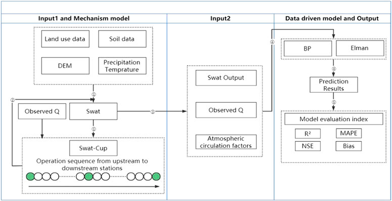
FIGURE 1. Technical roadmap of the coupling model.

Modeling steps for the coupling model.

(1) Data processing: we standardized the land use (remote sensing monitoring data for the land use status in China in 2015) and soil data (extracted from the Chinese soil dataset in HWSD), and combined DEM (www.gscloud.cn).

(2) SWAT modeling: with the above input conditions, we built the SWAT model to simulate runoff in the study area and generate output files.

(3) SWAT Cup calibration: we imported the SWAT output file into SWAT Cup (2.1.4), modified the type and quantity of the basin calibration parameters according to their impacts on runoff (Table 1), and calibrated the basin. The final calibration parameters were generated based on the upstream-to-downstream components of the flow domain.

(4) Anti substitution: the final parameters calibrated by SWAT Cup were inversely substituted into the parameter modification process of SWAT modeling. The SWAT model was rerun to obtain the state variables that had a significant impact on watershed runoff (Table 2).

(5) Input data collation: the state variables and atmospheric circulation factors obtained from the output of the SWAT model were unified in a fixed format.

(6) Data-driven model construction:

TABLE 1

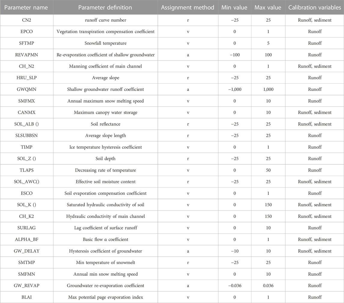
TABLE 1. Calibration runoff parameters.

TABLE 2

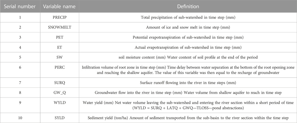
TABLE 2. Runoff impact state variables.

Firstly, the number of input layers is set to 1, indicating the input variables for the model. Similarly, the number of hidden layers is set to 1, determining the intermediate processing layers of the model. Lastly, the number of output layers is also set to 1, representing the predicted output variable. Additionally, an exclusive component, known as the take-up layer, is incorporated into the Elman networks.

Furthermore, the model is subjected to a predetermined number of network runs, specifically 10,000 runs in this study. This implies that the model terminates either when the predicted result reaches the optimal value within 10,000 runs or after 10,000 runs, irrespective of the attained result. Such an approach ensures a balance between convergence speed and accuracy during the model training process.

Moreover, the output error threshold of the model is set at 20%. This threshold serves as a criterion to trigger the back propagation algorithm, where the node weights and thresholds are adjusted iteratively to minimize the error. The model is then rerun until the desired results are achieved, indicating the attainment of the desired level of accuracy.

7) Model prediction effect and model performance evaluation: as shown in the last step of the technical framework in Figure 1, we used R2, MAPE, NSE, Bias, and other parameters for the model prediction results and model performance evaluation indicators. A comparison of the prediction results of the coupling model, SWAT model, BP neural network model, and Elman neural network model showed that the coupling model had a better prediction effect and was stronger and more stable (three parts).

2.2 SWAT model

The SWAT model (Arnold et al., 1998) was mainly developed in three stages. In the first stage, the United States Department of Agriculture (USAD) developed chemical runoff and erosion from agricultural management systems (CREAMS) in the 1970s with respect to the SWRRB model, which can simulate the impact of land use on the loss of sediment and chemical substances produced by agriculture. In the second stage, in the 1980s, to improve water quality evaluations in the simulation process, the groundwater loading effects on agricultural management systems (GLAMS) model, which can mainly describe the impact of chemicals in water on agricultural systems, was introduced to the SWRRB model. At this point, the SWRRB model could evaluate and analyze small watershed scale non-point source pollution under complex agricultural management measures, but it was not reliable for large-scale watershed simulations. In the third stage, in the 1990s, according to actual demand, the SWRRB model was combined with the roto (routing output to outlet) model, which can divide a basin into several sub-basins and directly collect runoff and sediment at the outlet of the entire basin, i.e., the SWAT model.

The SWAT model has been extensively modified and expanded, i.e., hydrological response units, such as runoff generation, infiltration, evaporation, and other hydrological processes have been added. This model also facilitates the direct input of rainfall, temperature, wind speed, and other meteorological data. It was initially used to simulate the loss of sediment and agricultural chemicals, but its functions in hydrological simulations have gradually expanded to areas such as watershed runoff. SWAT simulation is a distributed hydrological model that simulates the movement of water, sediment, and nutrients in a basin on daily, monthly, and annual scales based on GIS while relying on complex and variable land use and soil types.

During runoff simulation of a watershed, the distributed hydrological model includes two components: controlling the input of water, sediment, and chemical substances, among others, in the main river channel in each sub-watershed and determining the movement of water from the river network to the outlet of the watershed. The former mainly involves runoff generation and slope confluence, whereas the latter mainly involves the river confluence. The SWAT model follows the basic water balance equation in the overall simulation process:

$S{W}_t={SW}_0+{\displaystyle \sum _{i=1}^t}\left(R_{day}-Q_{surf}-E_a-W_{seep}-Q_{gw}\right)(1)$

where $S{W}_t$ represents the final moisture content of the soil, ${SW}_0$ represents the initial water content of the soil, t represents time, $R_{day}$ is precipitation, $Q_{surf}$ represents surface runoff, $E_a$ represents the evaporation capacity, $W_{seep}$ represents the amount of water entering the aeration zone in the soil profile, and $Q_{gw}$ is the water volume of the underground return flow.

The specific modeling process for the SWAT model is as follows.

1) Pre modeling preparation: before modeling, we prepared the basin regional elevation data layer (DEM data), regional land use data, soil type data, and meteorological data required for the modeling process.

2) Automatic watershed division: we performed automatic division of specific watersheds to form sub-watersheds and hydrological response units. We then calculated the area of the different sub-watersheds.

3) Hydrological response unit analysis: we matched the land use data and soil type data prepared in step 1) with the divided hydrological response unit in step 2) to simulate the environment in the watershed during an actual situation. We analyzed the slope classification in the basin.

4) Input meteorological data: we mainly used rainfall, temperature, wind speed, and other data as input. The simulation data from the SWAT model were used. At the same time, measured data can also be prepared and imported according to the format required by the model for watershed runoff simulation.

5) Operation and verification: we run the model to obtain the results and verified these using the SWAT Cup software. The parameters obtained after verification were input again into the SWAT model to determine the simulation effect and optimal parameter value.

The SWAT Cup software mentioned in step 5) in the SWAT modeling process was mainly used to calibrate and test the data after SWAT operation. The SWAT Cup software calibrates and tests the traffic at designated stations by setting parameters, providing a series of data useful for subsequent research, such as the simulated traffic, Nash coefficient, and optimal parameters. Both the SWAT and SWAT Cup versions used in this study are from 2012.

2.3 Data-driven model

2.3.1 BP neural network model

Rumelhart (1986) proposed the BP neural network, which has subsequently developed rapidly. At present, this neural network has been applied in various fields. Particularly, the application of the BP neural networks in the hydrological industry has opened new avenues for hydrological predictions. As a model simulating the human neural network, the BP neural network has a multi-layer network structure (including a three-layer network topology, i.e., the input layer, hidden layer, and output layer) (Nong ZhenXue, 2018) and multiple neurons, which can map the complex nonlinear relationship among input data. The self-learning characteristic of the BP neural network is that error is propagated forward and the weights among the input layer and middle layer and middle layer and output layer are corrected according to this error. Therefore, the output result is closer to the observed value (the end of model training was divided into two categories). The first category, within the training times set by the model, had an output error within the allowable error and the model terminated training. The second category showed that the model exceeded the set training times, but the error still exceeded the allowable error; thus, the model terminated the training. The number of model training processes should not be excessive; otherwise, the simulation results would be overfitted (The number of model training events is generally set to 3,000–10,000). The BP neural network was set as follows: three-layer network topology, two hidden layer nodes, 10,000 training processes, and an allowable error within 20%.

2.3.2 Elman neural network model

The Elman neural network (Fan Jieqing, 2019) was first proposed by J.L. Elman in 1990 to manage voice problems. The Elman neural network is a special recurrent neural network. In addition to the input layer, hidden layer, and output layer, the Elman model also includes a special hidden layer (also known as a correlation layer). The correlation layer and each hidden layer node have a corresponding correlation layer node. Therefore, the correlation layer can accept the feedback signal from the hidden layer and take the feedback signal received at the previous time, together with the current network input as the input for the hidden layer, to locally adjust the connection weight between the hidden layer and correlation layer of the model. This significantly reduces the feedback process in the model and improves the operation efficiency of the model. To ensure better model comparability, the Elman neural network model was consistent with the BP neural network model in terms of its parameter settings.

2.4 Model evaluation

In this study, four parameters, i.e., the determination coefficient (R2) (Cristiano, 2019), average value for the absolute value of the relative percentage error (MAPE), overall deviation rate (RBIAS) (Salas et al., 2000; Wang Jia, 2020) and Nash coefficient (NSE) (Nash and Sutcliffe, 1970), were used as the evaluation indicators [Eqs. 2–5. Among these, R2 was divided into linear regression and nonlinear regression. The closer the linear regression value is to 1, the better the simulation effect of the model. In contrast, the effect was poor. In nonlinear regression, the value may be greater than 1. The smaller the MAPE value, the better the prediction effect of the model; otherwise, the prediction result is poor. The smaller the RBIAS value, the better the prediction effect of the model. The NSE was divided into three components, approaching 1, approaching 0, and significantly less than 0, to evaluate the model. When the NSE infinitely approaches 1, the simulation effect of the model is the best and the model is the most reliable. When the NSE infinitely approaches zero, the simulation result was close to the average value of the measured value, i.e., the overall prediction result was credible, but the error in the simulation process was large. When the NSE was significantly less than zero, the simulation effect of the model was poor, i.e., the model was not credible:

$R^2=\frac{{\left[{\displaystyle \sum _{i=1}^n}\left(Q_{sim,i}-Q_{simavg}\right)\left(Q_{obs,i}-Q_{obsavg}\right)\right]}^2}{{\displaystyle \sum _{i=1}^n}{\left(Q_{sim,i}-Q_{simavg}\right)}^2{\displaystyle \sum _{i=1}^n}{\left(Q_{obs,i}-Q_{obsavg}\right)}^2}(2)$

$MAPE=\frac{1}{n}{\displaystyle \sum _{i=1}^n}\frac{\left(Q_{sim,i}-Q_{obs,i}\right)}{Q_{obs,i}}(3)$

$R_{BIAS}={\displaystyle \sum _{i=1}^n}\left(\frac{Q_{sim,i}-Q_{obs,i}}{Q_{obs,i}}\right)(4)$

$NSE=1-\frac{{\displaystyle \sum _{i=1}^n}{\left(Q_{obs,i}-Q_{sim,i}\right)}^2}{{\displaystyle \sum _{i=1}^n}{\left(Q_{obs,i}-Q_{obsavg}\right)}^2}(5)$

where n represents the number of runoff series, $Q_{sim,i}$ represents the ith simulated runoff, $Q_{simavg}$ represents the average value of all simulated runoff values, $Q_{obs,i}$ represents the observed runoff of the ith event, and $Q_{obsavg}$ represents the average value of the observed runoff.

Referring to the model performance classification rating proposed by Noori, N., Kalin et al. (2020), the following modifications were made in this study:

Very good: NSE ≥0.70; RBIAS ≤0.25.

Good: 0.70 > NSE ≥0.50; 0.25 < RBIAS ≤0.50

Satisfactory: 0.50 > NSE ≥0.30; 0.50 < RBIAS ≤0.70.

Unsatisfactory: NSE <0.30; RBIAS >0.70.

3 Case study

3.1 Study area

The Hanjiang River Basin, also known as the Mianyang water in ancient times, is located at 30°8′–34°11′N and 106°12′–114°14′E. The Hanjiang River Basin is the largest tributary of the Yangtze River, with a total length of 1,577 km, and spans six provinces: Hubei, Shanxi, Henan, Sichuan, Chongqing, and Gansu. The economic and social development of the Hanjiang River Basin is based on transportation. The Hanjiang River Basin belongs to a subtropical monsoon climate zone, with a humid climate and abundant water sources, but the climatic distribution is uneven throughout the year, mainly from May to October. Figure 2 shows the location and map of the Hanjiang River Basin.

FIGURE 2

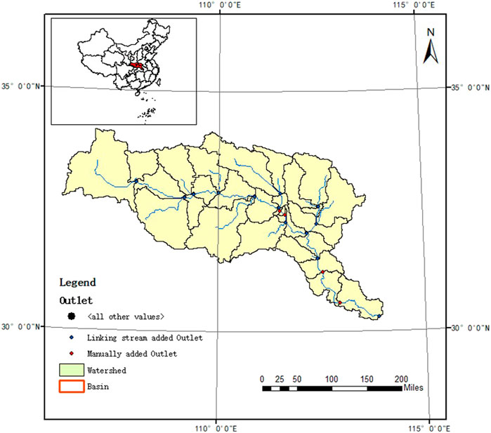
FIGURE 2. Location and map of the study area in China.

3.2 Model input

In this study, we primarily employed the SWAT mechanism model, as well as the data-driven models of BP neural network and Elman neural network. The SWAT model, serving as a mechanism-based approach, enables the simulation of various hydrological processes within the basin, including runoff generation and flow concentration. On the other hand, the BP neural network and Elman neural network models, as data-driven techniques, effectively handle the intricate nonlinear relationships among the input conditions. Consequently, the input conditions of the model can be categorized into three distinct components, benefiting from the combined strengths of these modeling approaches. Part I: The SWAT model was employed to simulate vital hydrological processes, encompassing runoff generation and fow concentration. The inputs essential for constructing the SWAT model primarily comprise high-resolution DEM data accurate to 30 m, land use data depicted in Figure 3, and soil type data illustrated in Figure 4. Among these, precipitation and other meteorological data were mainly obtained from the China Meteorological assimilation driving datasets for the SWAT model (CMADS) within the SWAT model of the China Meteorological assimilation system (CLDAS). The daily maximum temperature, daily minimum temperature, wind speed, wind direction, sunshine, and other meteorological conditions were derived from the world weather database (CFSR).

FIGURE 3

FIGURE 3. Distribution of land use in the study area.

FIGURE 4

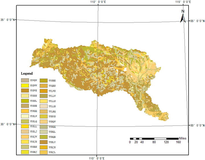
FIGURE 4. Distribution of soil types in the study area.

Part II: The input conditions, also referred to as predictors, were primarily utilized in the coupling model, which consisted of two main aspects: 1) extracted from the SWAT simulation results, which were modified and calibrated according to the parameters required for the SWAT Cup calibration proposed by Liu Lin et al. (2020); Ma Xinping et al. (2021); Zhang Chao (2020),; Zhu ZhengRu et al. (2021). In this study, as part of the input factors for the coupled model, 10 state variables were carefully selected following the simulation decomposition of the SWAT model. The names and definitions of these 10 state variables are provided in Table 2, presenting a comprehensive understanding of their significance in the analysis. 2) The input condition was not only the input condition of a single data-driven model but was also combined with (1) as the input condition of the coupled model. The input conditions included 130 atmospheric circulation factors (consisting of 88 atmospheric circulation indices, 26 SST indices, and 16 other indices), which were monitored by the National Climate Center of the China Meteorological Administration (http://cmdp.ncc-cma.net/Monitoring/cn_index_130.php).

To ensure the forecasting effectiveness of the coupled model, both the BP and Elman neural networks were employed in this study. The correlation between the forecast object and the predictors was calculated, and based on this analysis, 20 predictors with higher correlation were selected as the final input factors for the coupled model. Figure 5 presents the month-by-month correlation plots, showcasing the relationship between the predictors and the forecast object.

FIGURE 5

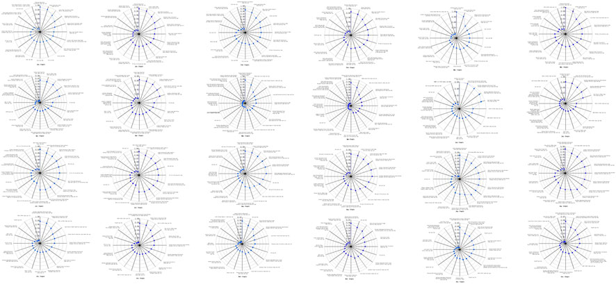
FIGURE 5. Correlation comparison of the monthly predictors between the coupled and single models: couple represent the coupled model for the SWAT and BP or Elman neutral network models. Single represents a single BP and Elman neutral network model. Both the BP and Elman neutral network analyzed the correlation between the runoff and atmospheric circulation factors, such that the selected factors were identical. In the figure WP is West Pacific Pattern, EA/WR is East Atlantic-West Russia Pattern. AAO is Antarctics Oscillation, NAO is North Atlantic Oscillation, AO is Arctic Oscillation, SCA is Scandinavia Pattern, PNA is Pacific/North America Pattern, NP is North Pacific Pattern.

The figure reveals that, compared to the period prior to the expansion of the influencing factors, the addition of state variables as influencing factors occurred in January, February, March, April, August, September, November, and December. In the remaining months, factors such as atmospheric circulation and runoff were consistently maintained as influencing factors. This observation suggests that the state variables exhibit varying degrees of influence during different months, thereby highlighting their seasonality and dynamic nature within the coupled model.

Part III: in addition to collecting, sorting, and analyzing the prediction factors, we also determined the observed runoff from upstream to downstream of the Hanjiang River Basin. These values were input in the third part of the model. We mainly collected and sorted the monthly runoff data for the Danjiangkou reservoir, Huangjiagang hydrological station, Huangzhuang hydrological station, and Xiantao hydrological station from 2008 to 2013 as the input conditions for the model. Data from the Danjiangkou reservoir, Huangjiagang hydrological station, and Huangzhuang hydrological station were mainly collected to calibrate the parameters of the runoff simulation in the Hanjiang River Basin. We then extracted the state variables required by the coupling model from its results. The data from Xiantao hydrological station were used for the experiment on runoff prediction in the study area.

4 Results and discussion

In order to demonstrate the superior applicability of the coupling model, separate predictions were performed using the BP neural network, Elman neural network models, and coupling models (SWAT + BP and SWAT + Elman) to forecast monthly runoff at the Xiantao station. The prediction results were then evaluated and analyzed comprehensively, taking into account both overall performance and month-to-month variations.

By conducting a thorough analysis of the prediction results, we aimed to provide a comprehensive understanding of the effectiveness and accuracy of each model, as well as to identify any potential variations in performance on a monthly basis. This approach allowed for a comprehensive evaluation and comparison of the different models, providing valuable insights into their respective strengths and limitations in predicting monthly runoff.

4.1 Analysis of overall runoff prediction results

To effectively analyze the accuracy and performance of the coupled models (SWAT + BP and SWAT + Elman) for runoff prediction at the Xiantao hydrological station, we constructed a runoff prediction diagram (Figure 6) for the individual BP neural network, Elman neural network models, and prediction results for the coupled model. We then calculated the evaluation parameter values for the prediction results of each model, as listed in Table 3. Based on the runoff prediction diagram of each model, the overall prediction effect of the BP neural network and Elman neural network was lower than that of coupling prediction model. Especially the fitting effect between the runoff prediction curve and observed runoff curve for the SWAT + Elman neural network model in the coupling models.

FIGURE 6

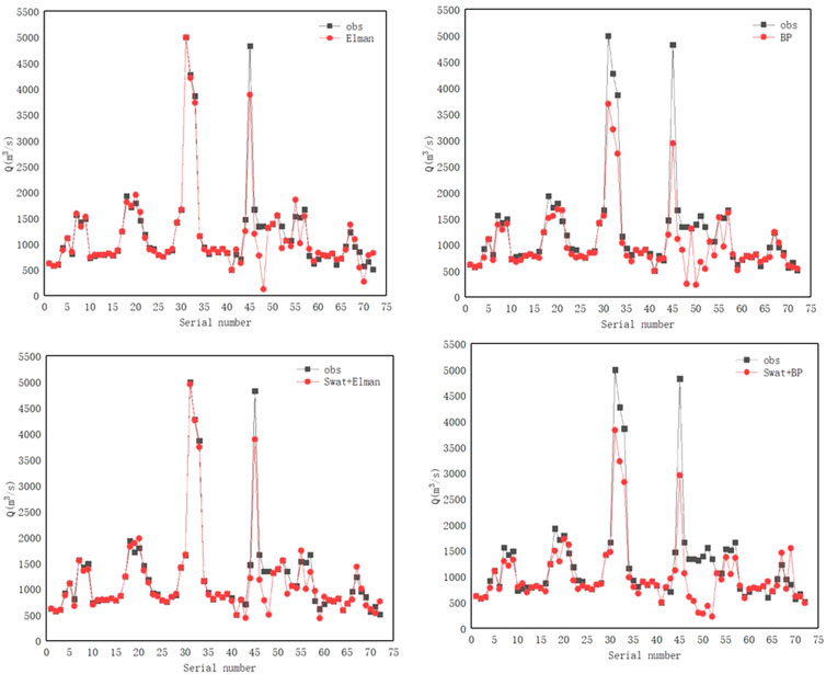
FIGURE 6. Fitting diagram for the runoff prediction curve and observed runoff curve of the four models at the Xiantao hydrological station.

TABLE 3

TABLE 3. Evaluation parameter values for the prediction results of various models at the Xiantao hydrological station.

The runoff prediction curve fitting chart only showed that the prediction effect of the coupled model was overall superior. This study introduced four parameters, i.e., the average of the absolute value for the relative percentage error (MAPE), overall deviation rate (RBIAS), and Nash coefficient (NSE), to evaluate the prediction results and performance of each model. According to the prediction results of each model for the runoff at the Xiantao hydrological station, we calculated the evaluation parameter values of each model, as listed in Table 3.

As shown in Table 3, the R_BIAS and MAPE of all models remained low in the validation period of the rate period, which indicates that the models have good predictions, while the NSE of the single Elman and BP neural network models were 0.93 and 0.8 in the rate period and 0.67 and −0.08 in the rate period, respectively, Elman had poor but acceptable predictions in the validation period, while the BP The prediction results of the neural network in the validation period indicate that the model structure is unstable, while the NSE of the coupled models SWAT+Elman and SWAT+BP in the rate period are 0.96 and 0.81, but in the validation period are 0.71 and 0.96, respectively, from the NSE results of the rate period and the validation period, the coupled models have a certain but small improvement in the NSE in the rate period compared with the single model. The NSE values of 0.71 and 0.96 for the coupled model in the validation period are much larger than those of 0.67 and −0.08 for the single model, indicating that the coupled model has better effectiveness, stability and robustness in the hydrological forecasting of the basin.

4.2 Analysis of monthly model prediction results

For the monthly runoff prediction results at the Xiantao hydrological station, we used the determination coefficient to perform a special evaluation. The closer the determination coefficient is to 1, the better is the prediction result of the model and the more stable is the performance of the model. Figure 7 shows the monthly runoff prediction map of the four models at the Xiantao hydrological station from January to December. The determination coefficient values of the Elman neural network, BP neural network, and coupling models (SWAT + Elman and SWAT + BP) are displayed in the upper left corner of each monthly prediction map. Based on Figure 7, the monthly prediction results for the Elman neural network, BP neural network, and coupling model tended to deteriorate with time; this was especially notable in November and December.

FIGURE 7

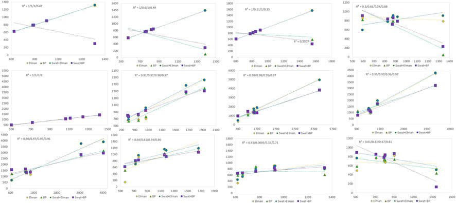
FIGURE 7. Monthly runoff prediction results and R² values at the Xiantao hydrological station. The closer the determination coefficient, R², is to 1, the better the prediction effect of the model and the more stable the model performance, and vice versa. In the figure, the y-axis represents the predicted flow and the x-axis represent the observed flow.

By observing the determination coefficient values of each model in Figure 7, we can conclude that the determination coefficients of the Elman and BP neural networks were high from the beginning to the end, resulting in a small space for improving the determination coefficients of the coupled model. Although the determination coefficient of the coupling model was low during individual months, overall, the determination coefficient of the coupling model was more stable, which also showed that the performance of the coupling model was more stable and reliable during the runoff prediction process.

Building upon the analysis presented above, this study introduces a novel concept and conducts a preliminary investigation into the coupling model. However, it is important to acknowledge that there is still a vast scope for future research and development in this field. The coupling model holds significant potential, and several avenues can be explored to advance its application and understanding.

(1) In future research, how to embed important hydrological processes such as flow production and sink into the data-driven model as a layer of neural structure of the model, i.e., to consider complex nonlinear relationships between important hydrological processes and different factors directly in the data-driven model to achieve deeper coupling.

(2) BP and Elman are more common data-driven models with functions such as complex nonlinear mapping. In the future research, Random Forest, Convolutional Neural Network, Long Short Term Memory Model and even Graph Convolutional Neural Network can replace these two models for coupling research.

(3) In this study, the predictors were screened by the correlation coefficient method (correlation analysis) when the input factors were finally determined, and the overall and month-by-month analysis of the prediction results was conducted. The analysis of the cyclical and seasonal effects of the predictors on the prediction results is lacking, and the authors will carry out the analysis of the cyclical and seasonal effects of the predictors on runoff to analyze the effects of the factors in more detail.

(4) There is a need to expand the application of the coupling model to different geographic regions and hydrological contexts. Testing the model’s performance in diverse environments can provide valuable insights into its generalizability and adaptability. Additionally, comparing the performance of the coupling model with other existing models can help identify its strengths and limitations.

(5) Exploring the potential integration of advanced technologies, such as remote sensing data, machine learning algorithms, and artificial intelligence, can further enhance the capabilities of the coupling model. These technologies can offer valuable data sources, improve predictive accuracy, and enable real-time monitoring and decision-making in hydrological forecasting.

In conclusion, while this study presents an initial exploration of the coupling model, it serves as a springboard for future research endeavors. Advancing the coupling model through improved accuracy, wider applicability, and integration of advanced technologies will contribute to more effective hydrological forecasting and decision-making processes.

5 Conclusion

In this study, we focused on evaluating the effectiveness of the coupling model for runoff prediction in the Hanjiang River Basin. By considering the prediction factors, we conducted a comprehensive analysis of the prediction results for the individual Elman neural network model, BP neural network model, and the coupled models (SWAT + Elman and SWAT + BP) both in terms of overall performance and on a monthly basis. The overall prediction results indicate a good fit for all models, with slight deviations observed in 2010 and 2012 as shown in Figure 6. To provide a clearer assessment of the advantages of the coupled models, the RBIAS, MAPE, and NSE indicators were employed to evaluate the forecasting performance of the models. The RBIAS and MAPE values of the models exhibited relatively small fluctuations and maintained stability in both the calibration and validation periods. In terms of NSE, the coupled models demonstrated comparable performance to the single model during the calibration period, while exhibiting higher stability in the validation period. Moreover, the NSE of the coupled model showed improvement compared to the calibration period, indicating enhanced prediction effectiveness and stability in forecasting.

Figure 7 presents the month-by-month prediction results, indicating that the coupled model achieves an R2 value greater than 0.7 in 70% of the months, greater than 0.8 in 67% of the months, and greater than 0.9 in approximately 42% of the months, approaching 50%. This suggests that the coupled model outperforms the single model in terms of month-by-month prediction, demonstrating superior performance and stability. Conversely, the R2 values of the single models exhibit a relatively wide range. Specifically, the Elman model spans from 0.01 to 1, while the BP model spans from 0.0005 to 1. This variation indicates a lack of stability in the prediction results of the single models.

Based on the investigation of runoff prediction and the analysis of prediction results for the Hanjiang River Basin, the following conclusions were drawn.

(1) The coupled model exhibited superior accuracy and reliability in runoff predictions within the watershed, surpassing the performance of single prediction models.

(2) The mechanism model plays a crucial role in improving the accuracy of watershed runoff prediction by simulating essential hydrological processes, including runoff generation and flow concentration. Through the decomposition of meteorological factors such as rainfall and the consideration of soil and watershed base flow conditions, the mechanism model generates state variables that greatly contribute to enhancing the accuracy of watershed runoff predictions.

(3) Through the analysis of overall and month-by-month forecasting effects, it has been demonstrated that the coupled model exhibits superior forecasting capabilities and stability. Furthermore, it demonstrates a high level of generalizability.

Data availability statement

The datasets presented in this article are not readily available because not have. Requests to access the datasets should be directed to GD 625613932@qq.com.

Author contributions

GD is the author of the idea and the main writer of the paper. HW, XL, CW, and XZ are mainly responsible for helping the improvement of the idea and the modification of the paper. LX and Li permit are mainly responsible for the modification of the figures and tables and for assisting me in data sorting. PS, YJ, and RY are mainly responsible for assisting me in sorting out the ideas, data processing and some simple drawing work. All authors contributed to the article and approved the submitted version.

Funding

This study was supported by the Young Elite Scientists Sponsorship Program by CAST (grant number 2019QNRC001).

Conflict of interest

Author RY was employed by Power China Huadong Engineering Corporation Limited.

The remaining authors declare that the research was conducted in the absence of any commercial or financial relationships that could be construed as a potential conflict of interest.

Publisher’s note

All claims expressed in this article are solely those of the authors and do not necessarily represent those of their affiliated organizations, or those of the publisher, the editors and the reviewers. Any product that may be evaluated in this article, or claim that may be made by its manufacturer, is not guaranteed or endorsed by the publisher.

Supplementary material

The Supplementary Material for this article can be found online at: https://www.frontiersin.org/articles/10.3389/feart.2023.1185953/full#supplementary-material

References

Arnold, J. G., Srinivasan, R., Muttiah, R. S., and Williams, J. R. (1998). Large area hydrologic modeling and assessment Part I: Model development. JAWRA 34 (1), 73–89. doi:10.1111/j.1752-1688.1998.tb05961.x

CrossRef Full Text | Google Scholar

Cristiano, E., Veldhuis, M. C., Wright, D. B., Smith, J. A., and van de Giesen, N. (2019). The influence of rainfall and catchment critical scales on urban hydrological response sensitivity. Water Resour. Res. 55 (4), 3375–3390. doi:10.1029/2018wr024143

CrossRef Full Text | Google Scholar

Fan, J. Q., Liu, C., Lv, Y. J., Han, J., and Wang, J. (2019). A short-term forecast model of foF2 based on elman neural network. Appl. Sci. 9 (14), 2782. doi:10.3390/app9142782

CrossRef Full Text | Google Scholar

Gao, Y. M., Lei, J. M., Liu, S. P., Zhou, X. B., Lu, D. P., et al. (2021). Research on flood forecasting of small reservoirs based on LSTM deep neural network. Proc. 11th flood control drought relief Inf. forum, 163–170. doi:10.26914/c.cnkihy.2021.024874

CrossRef Full Text | Google Scholar

Harris, A., and Hossain, F. (2008). Investigating the optimal configuration of conceptual hydrologic models for satellite-rainfall-based flood prediction. IEEE Geosci. Remote Sens. Lett. 5 (3), 532–536. doi:10.1109/lgrs.2008.922551

CrossRef Full Text | Google Scholar

Ji, Z. S., Zhang, G. W., and Zhang, Z. L. (2021). Water level forecast of pingyao hydrological station in dongtiaoxi based on convolutional neural network. Water Resour. Power 39 (8), 4. doi:10.32629/hwr.v4i6.3111

CrossRef Full Text | Google Scholar

Jiang, S., Zheng, Y., and Solomatine, D. (2020). Improving AI system awareness of geoscience knowledge: Symbiotic integration of physical approaches and deep learning. Geophys. Res. Lett. 47 (13), e2020GL088229. doi:10.1029/2020gl088229

CrossRef Full Text | Google Scholar

Koutroumanidis, T., Sylaios, G., Zafeiriou, E., and Tsihrintzis, V. A. (2009). Genetic modeling for the optimal forecasting of hydrologic time-series: Application in Nestos River. J. Hydrol. 368 (1-4), 156–164. doi:10.1016/j.jhydrol.2009.01.041

CrossRef Full Text | Google Scholar

Liu, L., Li, J. F., Li, Z. L., and Zhao, C. L. (2020). Construction and applicability evaluation of SWAT model in the upper reaches of Fenhe River. People's Yellow River 42 (11), 6. doi:10.3969/j.Issn.1000-1379.2020.11.012

CrossRef Full Text | Google Scholar

Ma, X. P., Wu, T., and Yu, Y. Y. (2021). Study on runoff scenario prediction in the upper reaches of the Han River based on SWAT model. Remote Sens. land Resour.

Google Scholar

Nash, J. E., and Sutcliffe, J. V. (1970). River flow forecasting through conceptual models part I — a discussion of principles. J. Hydrol. 10 (3), 282–290. doi:10.1016/0022-1694(70)90255-6

CrossRef Full Text | Google Scholar

Nong, Z. X. (2018). Research on medium and long-term runoff forecast in Ganjiang River basin.

Google Scholar

Noori, N., and Kalin, L. (2016). Coupling SWAT and ANN models for enhanced daily streamflow prediction. J. Hydrol. 533, 141–151. doi:10.1016/j.jhydrol.2015.11.050

CrossRef Full Text | Google Scholar

Noori, N., Kalin, L., and Isik, S. (2020). Water quality prediction using SWAT-ANN coupled approach. J. Hydrol. 590, 125220. doi:10.1016/j.jhydrol.2020.125220

CrossRef Full Text | Google Scholar

Rumelhart, D., and Mcclelland, J. (1986). Learning and relearning in Boltzmann machines. Cambridge, Massachusetts, United States: MIT Press.

Google Scholar

Salas, J., and Markus, M. (2000). Streamflow forecasting based on artificial neural networks. Netherlands: Springer.

Google Scholar

Wang, J., Wang, X., Lei, X. H., Wang, H., Zhang, X. H., You, J. j., et al. (2020). Teleconnection analysis of monthly streamflow using ensemble empirical mode decomposition. J. Hydrol. 582, 124411. doi:10.1016/j.jhydrol.2019.124411

CrossRef Full Text | Google Scholar

Xu, G. Y., Zhu, J., Si, C. Y., Hu, W. B., and Liu, F. (2019). Combined hydrological time series forecasting model based on CNN and MC. Comput. Mod. 15 (11), 7. doi:10.3969/j.issn.1006-2475.2019.11.005

CrossRef Full Text | Google Scholar

Xu, Z., Mo, L., Zhou, J., Fang, W., and Qin, H. (2022). Stepwise decomposition-integration-prediction framework for runoff forecasting considering boundary correction. Sci. Total Environ. 851, 158342. doi:10.1016/j.scitotenv.2022.158342

PubMed Abstract | CrossRef Full Text | Google Scholar

Yao, C., Li, Z. J., Zhang, K., Zhu, Y. L., Liu, Z. Y., Huang, Y. C., et al. (2021). Fine-scale flood forecasting for small and medium-sized rivers based on Grid-Xinanjiang model. J. Hohai Univ. Nat. Sci. 49 (1), 19–25. doi:10.3876/j.Issn.1000-1980.2021.01.004

CrossRef Full Text | Google Scholar

Yaseen, Z. M., Jaafar, O., DeoKisi, R. C. O., Adamowski, J., Quilty, J., and El-Shafie, A. (2016). Stream-flow forecasting using extreme learning machines: A case study in a semi-arid region in Iraq. J. Hydrol. 542, 603–614. doi:10.1016/j.jhydrol.2016.09.035

CrossRef Full Text | Google Scholar

Zhang Chao, (2020). Runoff simulation of Shaying River basin based on SWAT model.

Google Scholar

Zhao, Q., Zhu, Y. L., Shu, K., Wan, D., Yu, Y., Zhou, X., et al. (2020). Joint spatial and temporal modeling for hydrological prediction. IEEE Access 8, 78492–78503. doi:10.1109/access.2020.2990181

CrossRef Full Text | Google Scholar

Zhao, W. B., Wang, X. N., Xiao, C. L., et al. (2021). Application of BP_adaboost model and xin’anjiang model of grouped modeling in flood forecasting of DHF reservoir basin. Water Resour. Power.

Google Scholar

Zhu, Z. R., Yuan, C., and Lv, L. T. (2021). Runoff simulation of Taizi River basin based on SWAT model. Liaoning, China: Journal of Liaoning Normal University: Natural Science Edition.

Google Scholar