A seamless approach for evaluating climate models across spatial scales

1 Introduction

Climate models serve as the fundamental technology enabling scientists to make predictions about future changes in Earth’s climate. Currently, many different types of models exist, including global climate models (GCMs), regional climate models (RCMs), and regionally refined models (RRMs). These models generate distinct simulations of the same planet and its climate. In particular, RRMs generate simulations at a finer spatial resolution over a specific region than the resolution for the rest of the globe (Randall et al., 2007; Ringler et al., 2008). There are several benefits to increasing the spatial resolution of climate models, the primary of which is being able to resolve and more accurately simulate smaller-scale processes such as convection and precipitation (Roberts et al., 2018). However, computational costs increase exponentially as model resolution increases. In particular, between RRMs and GCMs, it is currently unknown whether the benefits associated with higher model resolution outweigh the corresponding increases in computational power.

Increasing the resolution in climate models is absolutely necessary to accurately simulate the climate in some locations, however. Some regions of the world exhibit drastically more complex topography. These topographically complex regions often experience notable changes in weather and climates over short distances. Changes in topography are strongly correlated with variations in seasonality and key meteorological variables, including clouds, precipitation, and surface temperatures. In particular, precipitation is subject to topographical influences as there are orographic processes that can significantly increase the precipitation amounts on the windward sides of mountain ranges (and, conversely, decrease precipitation amounts on the leeward sides) (Minder and Roe, 2009). As a result, climate models may struggle to accurately reproduce these key variables such as precipitation in these topographically complex regions unless their spatial resolution is sufficiently high (Randall et al., 2007).

Most climate models with low resolution address that issue in topographically complex regions by employing parameterizations and downscaling techniques. For instance, simulating orographic precipitation can be achieved by employing a subgrid parameterization of surface elevation to appropriately enhance precipitation amounts on the windward sides of mountain ranges (Leung and Ghan, 1995). These techniques enable more accurate simulations of certain atmospheric processes while maintaining computational efficiency. However, many parameterization techniques fail to adequately resolve the inaccuracies inherent in climate model simulations with low spatial resolutions. Conversely, there are significant benefits of climate simulations at higher spatial resolutions, primarily in their improved ability to resolve complex topography (Palmer, 2014; Bador et al., 2020; Gutowski et al., 2020; Iles et al., 2020; Kim et al., 2022).

Recently, several GCMs have been developed with sufficiently high resolution. While high-resolution climate models provide more detailed information about Earth and its atmospheric processes, producing global simulations at such high spatial resolutions (e.g., 3 km or higher) remains infeasible due to the substantial computational costs associated with running, storing, and analyzing the massive output (Lupo et al., 2013). Additionally, because RRMs are relatively new, little prior analysis has been conducted to demonstrate the value added by regionally high spatial resolution in RRMs. As a result, it is currently unknown whether the benefits of high resolution in RRMs outweigh the increased computational costs they entail (Fu and Lee, 2022). Furthermore, there are very few frameworks available for the quantitative evaluation of the benefits of high-resolution models (Fu and Lee, 2022).

Recognizing the need, the primary scientific goal of this study is to develop a cross-disciplinary framework for quantifying the advantages of regionally high spatial resolutions in RRMs. The following sections outlines the development of the framework and its application to precipitation simulations. We compared the simulations of precipitation in GCMs, RRMs, and NASA’s satellite observations. The comparison results are used to justify the preference of RRMs (higher resolution) over GCMs (lower resolution). While this study does not aim to specifically compare precipitation simulations between models and observations per se, precipitation is a relatively straightforward variable to understand and compare across datasets of varying spatial and temporal resolution compared to other climate variables. As such, precipitation observations and simulations are chosen to evaluate the framework of focus in this study.

2 Data and methods

2.1 Raw data

There were three primary datasets used in this study. Two are from climate model runs, and the other is from NASA satellite observational data. The observational dataset used in this study is the NASA Global Precipitation Measurements Integrated Multi-Satellite Retrievals (GPM IMERG). Further details about the satellites and precipitation retrieval process can be found in Bolvin (2020). The GPM IMERG Final Run data were used in this study, and the data have a spatial resolution of 0.1° globally, or roughly 11 km. This resolution is higher than that of the data in both model runs. Only the total precipitation rate data (precipitationCal) are used for this study. The units of this variable are in millimeters per hour (mm/h).

The primary climate model simulations used in this study are from the Energy Exascale Earth System Model (E3SM) Version 2. Details about this model and its data can be found in Golaz et al. (2022), and only a brief overview is provided here. The low resolution (LR) and North American Regionally Refined Model (NARRM) runs from E3SM are used (Tang et al., 2023).

Both low resolution (LR) and North American Regionally Refined Model (NARRM) simulations from E3SM were used in the current study. While both datasets are based on output from the same E3SM, for the purposes of this study, the LR run is considered a GCM as it has a spatial resolution of approximately 100 km globally. Similarly, the NARRM run is considered an RRM as it has a spatial resolution of approximately 25 km, covering a significant portion of North America as shown in Figure 1, with 100 km spacing between grid points elsewhere. It should be noted that because some cloud parameterizations in E3SM suffer from poor scale-awareness, the NARRM adopts the hybrid timestep approach, i.e., a combination of low-resolution physics timesteps and the high-resolution dynamics timesteps, for the atmosphere model to achieve reasonable global climate for CMIP6 production simulations (Tang et al., 2023). Such choice should be taken into account when interpreting NARRM results relative to the LR counterpart. In these datasets, only the convective precipitation rate (PRECC) and stable precipitation rate (PRECL) data are used. The sum of PRECC and PRECL yields the total precipitation rate (PRECT). The units of these precipitation variables are all in millimeters per hour (mm/h).

FIGURE 1

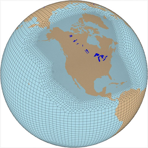
FIGURE 1. The E3SM v2 North American RRM grids reproduced from Figure 1b of Tang et al. (2023).

All three datasets were analyzed at three temporal scales: monthly, daily, and 3-hourly. Although the data are available for several years between 2000 and 2020, only the year 2014 is chosen as a representative year for the evaluation using the inter-resolution framework. The analyzed simulated and observed data amounted to approximately 233 gigabytes.

In addition to climate model datasets, elevation data from the Joint Institute for the Study of the Atmosphere and Ocean (JISAO) were used. These elevation data primarily served to assess the topographical complexity of various regions within CONUS (Mitchell, 2014).

This analysis focuses on the precipitation of the continental United States (CONUS), which encompasses the region between −130° and −60° longitude and 20°–60° latitude.

2.2 HEALPix

Due to the significant disparities in spatial resolutions among the three datasets, quantitative comparisons necessitate the regridding of the data to common resolution and pixels. As the E3SM RRM run contains irregularly spaced grid points in part of its simulations, a specific regridding process is necessary for this study. Consequently, the datasets are remapped onto the Hierarchical Equal-Area isoLatitude Pixelization (HEALPix) pixels at the respective spatial resolutions (Górski et al., 2005). HEALPix is a rearrangement of spherical model data that essentially simplifies the comparisons between models and observations of different spatial resolutions. The details of the mathematics behind how the data are rearranged and interpolated are outlined in Górski et al. (2005). This pixelization has been used in several cosmology and engineering studies such as Gao et al. (2019), Krachmalnicoff and Tomasi (2019), and Fernique et al. (2015). However, HEALPix has largely remained unused in atmospheric science and climate studies despite the fact that the pixelization is designed for spherical mediums such as Earth’s atmosphere.

HEALPix possesses several important properties that are pertinent to this research. Firstly, at any given spatial resolution, all pixels have equal areas (Górski et al., 2005). This characteristic mitigates the problem of spherical distortion encountered in Cartesian grids. Secondly, the conversion between different spatial resolutions in HEALPix merely entails a straightforward partitioning of pixels of lower-resolution pixels to form four nested pixels with higher resolution (Fu and Lee, 2022). The partitioning process preserves the geometric similarity of the grid points as illustrated in Figure 2. These two properties of HEALPix greatly simplify the comparison process among all remapped datasets. Once the data is in the HEALPix arrangement, it can be regridded to lower resolutions, as needed, using the aforementioned partition averaging process. Table 1 provides an overview of the HEALPix levels and the associated spatial resolutions (Górski et al., 2005).

FIGURE 2

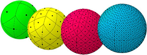
FIGURE 2. The HEALPix regridding/partitioning process (Górski et al., 2005).

TABLE 1

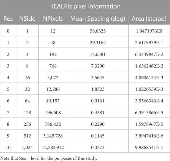
TABLE 1. HEALPix pixel information with levels and associated spatial resolution.

These properties of the HEALPix remapping make it the preferred framework compared to other remapping techniques used in other RCM studies. For example, Kalognomou et al. (2013) uses a bilinear interpolation remapping method, and Eum et al. (2011) uses a distance-based weighted average remapping method. These methods have simple calculations when using Cartesian-based grids on a sphere (as is the case for the models used in those studies). However, the calculations for remapping become rather complex when applied to the E3SM grid due to its nonuniform spacing as seen in Figure 1. As such, using HEALPix greatly simplifies the remapping process for models with irregularly-spaced non-Cartesian grids. Furthermore, because the previously-defined CONUS region has a relatively large meridional extent, any remapping techniques used have to account for the reduced surface area of grid points that are more poleward when computing overall statistics. The equal-area property of HEALPix simplifies this calculation and further justifies its use over other remapping frameworks.

In the HEALPix arrangement, the LR, NARRM, and GPM IMERG datasets have spatial resolutions of 203 km, 51 km, and 13 km, respectively. These are coarser spatial resolutions than those of the original data, but the reduction is necessary to allow for the appropriate comparisons between each of the datasets.

2.3 Metrics

Before discussing the metrics, it is important to address the topographical complexity of CONUS. This study defines topographical complexity by the spatial variance/standard deviation of the elevation, and a more topographically complex region will have a higher spatial variance in elevation.

There are several key climate model metrics analyzed in this study, each with a different purpose for analysis. The first metric is the bias in regionally averaged precipitation. This was chosen to evaluate the precipitation simulations in the regions with varying topographical complexity. In the current study, the CONUS was divided into seven different regions as defined in the United States National Climate Assessment: the Northwest (NW), Southwest (SW), Northern Great Plains (GPN), Southern Great Plains (GPS), Southeast (SE), Northeast (NE), and Midwest (MW) (USGCRP, 2018). The topographical complexity of each region, as well as which states the regions encompass, are shown in Figure 3. The spatially averaged precipitation values were calculated for each region, across the three temporal scales, and for each of the original dataset within the entire year of 2014. The HEALPix remapping was not used during the calculation of bias in regionally averaged precipitation.

FIGURE 3

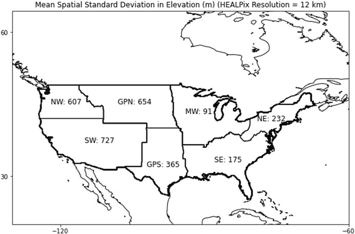
FIGURE 3. Regionally-Averaged Standard Deviation in Elevation over CONUS regions. This is a measure of topographical complexity.

Next, we analyze the distribution of precipitation rates using the Kolmogorov-Smirnov (KS) test at the 99% confidence level on the cumulative distribution functions (CDF). Each pair of datasets (LR vs. NARRM, LR vs. IMERG, NARRM vs. IMERG) is compared to obtain the KS test statistics. These statistics determine the similarity of the precipitation rate distributions across datasets, and also assess the presence of biases in the distributions of LR- and NARRM-simulated precipitation. For this metric, the frequencies of precipitation rate values are calculated using the raw precipitation data across the entire spatial domain of CONUS and the temporal domain of year 2014. Since the data are discrete, Gaussian kernel density estimates are used to approximate the CDFs. HEALPix remapping was not implemented for these two metrics as the analysis of the raw precipitation data is necessary to assess the effects of predicted precipitation bias.

Furthermore, we assess how the spatial variance in precipitation changes with different HEALPix resolution levels. The purpose of this metric is to highlight the extent to which spatial variability of precipitation increases as spatial resolution improves. The HEALPix-remapped data for all three datasets are regridded to each of the coarser HEALPix spatial resolution levels. At each HEALPix level, the spatial variance of precipitation is calculated over the CONUS domain. This process is repeated for the seven regions to assess any regional differences or topographical effects.

From there, we compare the HEALPix resolution levels to the relative change in spatial variance of precipitation. This metric offers insight into the value of higher-resolution climate simulations. Mathematically, it is calculated by taking the spatial variance in precipitation at each HEALPix spatial resolution level and computing the difference in variance values between a given HEALPix level and the previous level. The difference values are then divided by the variance value of the previous HEALPix level. The resulting proportions represent the relative percent decrease in spatial variance of precipitation between a given HEALPix level and the previous level. This process is repeated for the seven regions.

Lastly, we assess the differences in spatial variance of precipitation between model simulations and observations. This metric directly evaluates the performance of the precipitation simulations compared to observations. Mathematically, it is calculated by dividing the spatial variance in precipitation of both E3SM remapped datasets by the spatial variance in precipitation of the GPM IMERG remapped dataset. The resulting proportions indicate the percentages of observed spatial variance of precipitation explained by E3SM simulations. This is performed over the whole CONUS domain and the seven regions.

It should be noted that the temporal domain of 2014 is not identical between the model run data and the observational data; The E3SM simulations for the year 2014 do not precisely replicate the observed precipitation conditions for a given temporal instant in that year. As such, the raw spatial precipitation rate maps at specific temporal moments will appear significantly different between E3SM runs and GPM IMERG. However, it is worth mentioning that all of the aforementioned metrics involve some form of temporal averaging in some way, and the metrics primarily focus on the climatological aspects of CONUS precipitation. Therefore, it is acceptable to make comparisons between E3SM and GPM IMERG despite the disparity in temporal alignment.

3 Results

3.1 Regionally averaged precipitation

The results of Regionally Averaged Precipitation, shown in Figure 4, exhibit regional variations. In the NW, SW, and GPN regions, both E3SM simulations show that the spatiotemporal mean precipitation rates are 1 and 2 times higher than those of GPM IMERG. Conversely, in the SE region, spatiotemporal mean precipitation rates in both E3SM runs are approximately 70%–90% of the GPM IMERG precipitation rate. For the NE, MW, and GPS regions, both E3SM simulations capture the spatial-temporally averaged precipitation well, with differences between simulated and observed precipitation rates not exceeding 20%.

FIGURE 4

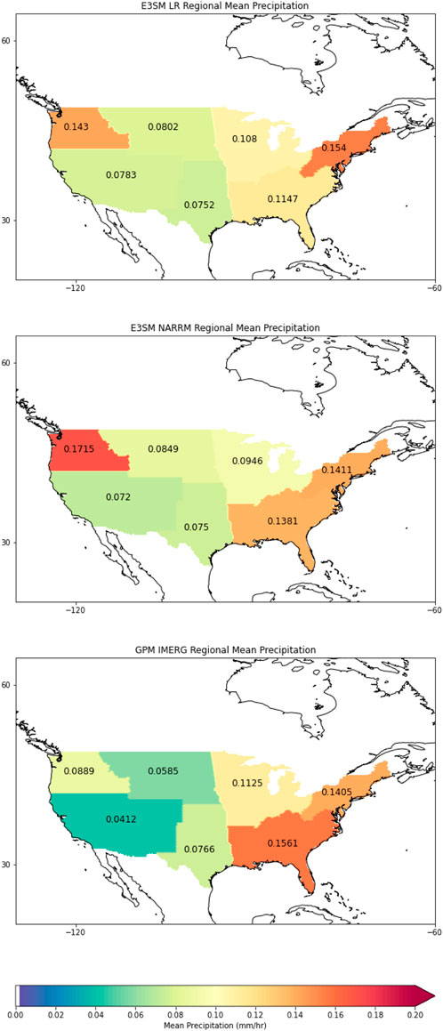
FIGURE 4. Regionally averaged precipitation rates (3-hourly temporal scale).

3.2 Kolmogorov-Smirnov test on precipitation rate distribution

The results of the KS tests are presented in Table 2. Notably, for all temporal resolutions, the test statistics values are lower for E3SM NARRM vs. GPM IMERG compared to E3SM LR vs. GPM IMERG. This indicates that E3SM NARRM captures the observed precipitation rate distribution more accurately than E3SM LR. This result is not surprising considering the inherent resolution differences between the two model runs. It should be noted that all KS test statistics are significant at the 99% confidence level, and the corresponding p-values are provided in Table 3.

TABLE 2

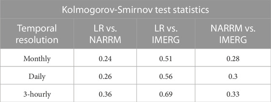
TABLE 2. Kolmogorov-Smirnov test statistic values between precipitation distributions.

TABLE 3

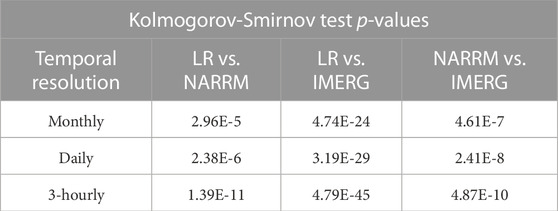
TABLE 3. Kolmogorov-Smirnov test p-values between precipitation distributions.

For reference, the probability distribution function (PDF) and cumulative distribution function (CDF) of all datasets are shown in Figure 5. Two additional results are worth highlighting. Firstly, as shown in the PDFs, E3SM LR simulates a significantly lower frequency of higher precipitation rates than E3SM NARRM does, and E3SM NARRM also exhibits lower frequencies of higher precipitation rates than GPM IMERG. This result is expected given that the difference in spatial resolution, with GPM IMERG having the highest and E3SM LR having the lowest resolution among the three datasets. This pattern holds true at the monthly, daily, and 3-hourly scales. Additionally, increasing the temporal resolution leads to an overall increase in the frequency of all precipitation rates, regardless of the dataset.

FIGURE 5

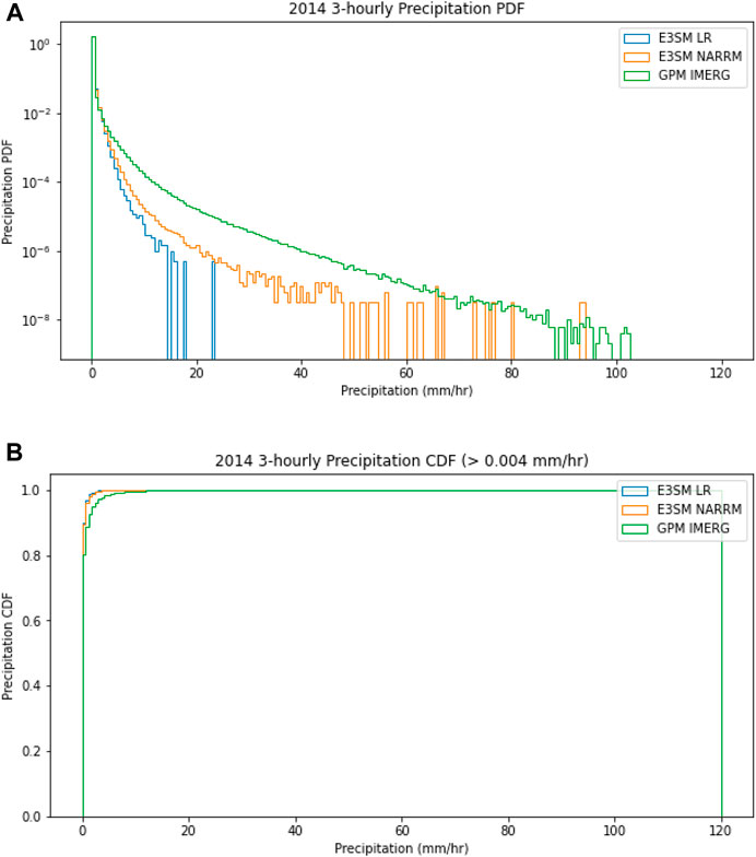
FIGURE 5. (A) Probability distribution function of total precipitation rates (3-hourly temporal scale). (B) Cumulative distribution function of total precipitation rates (3-hourly temporal scale).

The second additional result involves the CDFs of the three datasets. Specifically, at lower precipitation rates, the CDF values in both E3SM datasets are lower than those of GPM IMERG, before converging closer to each other at high precipitation rates. This indicates that the E3SM runs simulate a higher proportion of lower precipitation rates compared to observations. Again, the pattern holds true at each of the monthly, daily, and 3-hourly temporal scales. This bias is common in many climate models, and E3SM is no exception. Further details about this bias are discussed in Pendergrass and Hartmann (2014) and Taylor et al. (2022).

3.3 Spatial variance in precipitation vs. spatial resolution

There are two important results to highlight from analyzing the sensitivity of the spatial variance in precipitation with respect to spatial resolution. These are shown in Figure 6. Firstly, in both models and observations, as the HEALPix level and spatial resolution increase, so does the spatial variance in precipitation. While this result is not surprising, the slopes of the line plots in the figures provide insight into the extent of additional spatial information is captured in precipitation simulations with higher spatial resolutions. Similarly, when examining temporal resolution, the variance increases as temporal resolution increases. This trend holds true when considering the seven regions within CONUS.

FIGURE 6

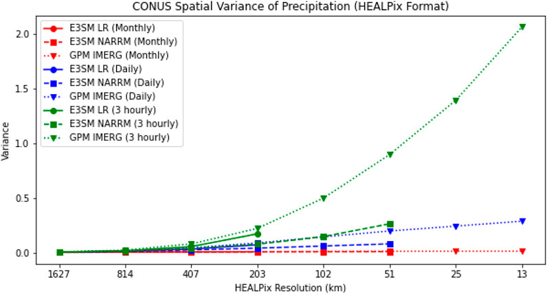
FIGURE 6. CONUS spatial variance of total precipitation rates vs. spatial resolution.

The second result pertains to the comparison between E3SM LR to E3SM NARRM. Despite having a higher HEALPix spatial resolution, the spatial variance in precipitation of the NARRM is lower than that of the LR. This pattern remains consistent across changes in spatial resolution, temporal resolution, and the CONUS regions. This result has implications for E3SM precipitation simulations, which will be discussed later.

3.4 Relative percentage change in spatial variance of precipitation vs. spatial resolution

The results for the relative change in spatial variance of precipitation between spatial resolutions, as depicted in Figure 7, highlight the importance of high-resolution simulations by themselves. As the spatial resolution increases, the increase in spatial variance from the previous spatial resolution level to the next decreases. Still, it is worth noting that spatial variance in precipitation increases by approximately 50% between 25 km and 13 km at the three-hourly temporal scale. The patterns hold consistent when considering changes in temporal resolution in all datasets, as well as changes in regional domains. All of these increases between spatial resolution levels demonstrate how higher spatial resolution capture additional spatial information about precipitation.

FIGURE 7

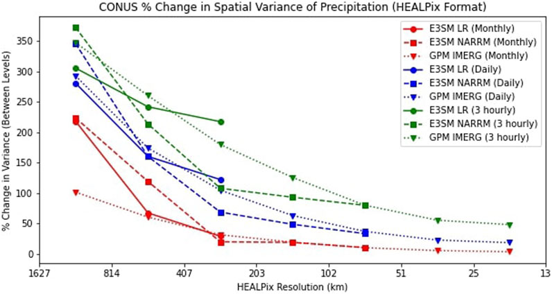
FIGURE 7. CONUS relative % change in spatial variance of total precipitation rates vs. spatial resolution.

3.5 Percentage of observed spatial variance in precipitation vs. spatial resolution

Results for this metric are shown in Figure 8. The first notable result here is that the percentage of spatial variance in precipitation explained by models generally decreases as spatial resolution increases across all temporal scales, except for 407 km resolution at the monthly timescale. However, the pattern generally flips when analyzing the seven CONUS regions individually, where models explain more variance in precipitation at the higher spatial resolutions. The exception is the GPN region, where the trends are quite inconsistent with both temporal and spatial resolution changes. The second notable result is that despite having a higher spatial resolution than E3SM LR, E3SM NARRM explains less of the observed spatial variance in precipitation at all spatial resolutions, timescales, and in all of the CONUS regions. The implications of these results on the E3SM runs’ performance are discussed in the following section.

FIGURE 8

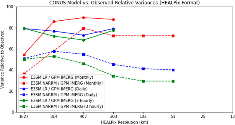
FIGURE 8. CONUS % of spatial variance of total precipitation rates explained by models vs. spatial resolution.

4 Conclusion

4.1 The new framework

In this study, a framework was developed for comparing model simulations and observations of different spatial resolutions. Multiple model and observational datasets were used, and they were regridded to the appropriate HEALPix resolution as needed. This regridding allowed for quantitative comparisons of precipitation between the datasets at different spatial resolutions. This framework was tested on the E3SM LR and E3SM NARRM model runs, as well as the GPM IMERG observations, which have significantly different spatial resolutions. The remapping onto the HEALPix pixels was necessary to compare the three datasets. This remapping process greatly simplified the comparisons between all three datasets as it standardized not only a common spatial resolution but also a common layout and/or arrangement for all the data. HEALPix enabled the inter-resolution comparisons that would have otherwise been mathematically challenging.

Several metrics were calculated to evaluate the precipitation from E3SM model against GPM IMERG observations. The primary objective is to determine the viability of this framework in comparing multiple datasets with different native spatial resolutions. The chosen metrics were relevant for evaluating the HEALPix framework’s viability. While some results regarding E3SM’s performance may seem counterintuitive in the context of climate model development, this study’s findings demonstrate that the framework produced meaningful results for comparing E3SM LR, E3SM NARRM, and GPM IMERG despite their significant differences in their native resolutions. The successful application of this framework opens up possibilities for its use in other climate model versus observational comparisons, particularly for inter-resolution comparisons.

4.2 E3SM

As aforementioned, several results about E3SM’s performance showed that the E3SM RRM performs worse than the E3SM LR in CONUS precipitation simulations. Firstly, the RRM has a lower spatial variance in precipitation than the LR at all resolutions. Furthermore, the RRM explains less of the observed precipitation variance than the LR. This is because the NARRM is developed for climate production campaigns (e.g., CMIP6), hence, it needs to meet the criteria of reasonably simulating global climate. NARRM adopted the hybrid time step method (i.e., a combination of an LR physics time step and the high-resolution dynamics time steps) in the atmosphere model to achieve the reasonable global performance without sacrificing too much of the benefits from high-resolution dynamics (Tang et al., 2023). The hybrid time step approach cannot take full advantage of the high-resolution dynamics at 25 km due to large time-truncation errors. Additionally, 25 km spatial resolution is not sufficiently high enough to accurately simulate small-scale precipitation features. To accurately represent these small-scale processes, a much higher spatial resolution, typically around 4 km or higher, is often required, and model parameterizations must be set appropriately to account for any spatial coarsening effects. Consequently, the 25 km resolution of the RRM resulted in a lack of spatial variance that would otherwise be present in simulated precipitation at a higher resolution than 25 km. Any small-scale precipitation features present in the RRM are effectively filtered out when remapping to coarser resolutions, and this has the effect of generally lowering the spatial variance in precipitation.

In both of the E3SM simulations, as the spatial resolution (HEALPix Level) increases, the observed spatial variance in precipitation explained by both model runs also decreases. This result can be attributed to the E3SM’s ability to simulate larger-scale precipitation features such as atmospheric rivers, cold fronts, and monsoonal systems. The 100 km spatial resolution of the LR may be sufficiently high enough to accurately simulate these large-scale precipitation features. As such, simulating these features in the RRM at 25 km resolution did not significantly contribute to the overall spatial variance since there was minimal additional information gained by simulating these large-scale features at a higher resolution.

In conclusion, when considering total precipitation simulations, the advantages of increasing the spatial resolution in the E3SM RRM generally do not outweigh the drawbacks in terms of increased computational costs. The RRM’s 25 km resolution may not be high enough to accurately capture small-scale precipitation processes, while the LR already performs well in simulating larger-scale precipitation features at its resolution. Because E3SM performs better in simulating large-scale precipitation features than simulating small scale-features, increasing the HEALPix resolution would ultimately decrease the proportion of observed precipitation variance that E3SM explains because the added resolution would not be able to sufficiently explain the small-scale precipitation features that become increasingly more present as HEALPix resolution increases.

4.3 Next steps

Overall, this research has laid the foundation for comparing models and observations across different spatial scales, demonstrating the viability of the developed framework. Indeed, the counterintuitive results obtained in this study regarding E3SM precipitation simulations should not be generalized to all variables, climate models, or regions outside of the CONUS. It is important to recognize the complexity of climate modeling and the wide range of factors that can influence model performance. Moving forward, there are several promising avenues for further research. Expanding the analysis to include other variables simulated by E3SM or other climate models would provide a more comprehensive understanding of the model’s performance across different spatial resolutions. Additionally, extending the study beyond the CONUS to different regions would help assess the generalizability of the findings. To better evaluate the computational costs associated with analyzing datasets, developing quantifiable metrics is crucial. Incorporating these metrics into the research would enable comparisons of computational costs between different datasets and facilitate a more accurate cost-benefit analysis. This analysis would help determine whether the benefits of high-resolution climate model simulations outweigh the drawbacks in terms of computational power.

Data availability statement

The original contributions presented in the study are included in the article/Supplementary Material, further inquiries can be directed to the corresponding author.

Author contributions

AC contributed to the data curation, formal analysis, investigation, methodology, validation, visualization, and writing (all parts) of this project. HL contributed to the conceptualization, funding acquisition, project administration, resources, software, supervision, validation, and writing (editing/review) of this project. RF contributed to the conceptualization, funding acquisition, project administration, resources, software, supervision, validation, and writing (editing/review) of this project. QT contributed to the data curation, resources, software, and writing (editing/review) of this project. All authors contributed to the article and approved the submitted version.

Funding

This study was funded by the Joint Institute for Regional Earth System Science and Engineering (JIFRESSE) and the National Science Foundation (NSF) under grants 1917781 and AGS-2214697.

Acknowledgments

This study was made possible courtesy of the following additional parties: The National Aeronautics Space Administration (NASA), who made the GPM IMERG dataset available for use in this study. The Atmospheric and Oceanic Sciences (AOS) Department of UCLA, who provided the necessary computational resources to produce the results of this study. The Regional Climate Modeling Evaluation System (RCMES) group of the Jet Propulsion Laboratory (JPL), who provided plenty of relevant feedback on the results of this study. HL’s contribution to this work was performed at JPL, California Institute of Technology, under a contract with NASA. We thank NASA’s Advanced Information Systems Technology award (21-AIST21_2-0020) for supporting this work. Lawrence Livermore National Laboratory (LLNL) is operated by Lawrence Livermore National Security, LLC, for the U.S. Department of Energy (DOE), National Nuclear Security Administration under Contract DE-AC52-07NA27344. Support has been received from the Energy Exascale Earth System Model (E3SM) project, funded by the U.S. Department of Energy, Office of Science, Office of Biological and Environmental Research (BER) and the LLNL LDRD project 22-ERD-008, “Multiscale Wildfire Simulation Framework and Remote Sensing”. E3SM production simulations were performed on a high-performance computing cluster provided by the BER Earth System Modeling program and operated by the Laboratory Computing Resource Center at Argonne National Laboratory, and the National Energy Research Scientific Computing Center (NERSC), a DOE Office of Science User Facility supported by the Office of Science of the U.S. Department of Energy under Contract No. DE-AC02- 05CH11231.

Conflict of interest

The authors declare that the research was conducted in the absence of any commercial or financial relationships that could be construed as a potential conflict of interest.

Publisher’s note

All claims expressed in this article are solely those of the authors and do not necessarily represent those of their affiliated organizations, or those of the publisher, the editors and the reviewers. Any product that may be evaluated in this article, or claim that may be made by its manufacturer, is not guaranteed or endorsed by the publisher.

Supplementary material

The Supplementary Material for this article can be found online at: https://www.frontiersin.org/articles/10.3389/feart.2023.1245815/full#supplementary-material

References

Bador, M., Boé, J., Terray, L., Alexander, L. V., Baker, A., Bellucci, A., et al. (2020). Impact of higher spatial atmospheric resolution on precipitation extremes over land in global climate models. J. Geophys. Res. Atmos. 125, e2019JD032184. doi:10.1029/2019JD032184

CrossRef Full Text | Google Scholar

Bolvin, D. T. (2020). Imerg v06 technical documentation. United States: NASA.

Google Scholar

Eum, H.-I., Gachon, P., Laprise, R., and Ouarda, T. (2011). Evaluation of regional climate model simulations versus gridded observed and regional reanalysis products using a combined weighting scheme. Clim. Dyn. 38, 1433–1457. doi:10.1007/s00382-011-1149-3

CrossRef Full Text | Google Scholar

Fernique, P., Allen, M. G., Boch, T., Oberto, A., Pineau, F.-X., Durand, D., et al. (2015). Hierarchical progressive surveys. Astronomy Astrophysics 578, A114. doi:10.1051/0004-6361/201526075

CrossRef Full Text | Google Scholar

Fu, R., and Lee, H. (2022). “2022 jifresse summer internship program (jsip): announcement of opportunities,” in Apply data science to support ultra-high resolution climate model development using satellite data (United States: UCLA).

Google Scholar

Gao, Y., Du, Z., Xu, W., Li, M., and Dong, W. (2019). Healpix-ia: A global registration algorithm for initial alignment. Sensors 19, 427. doi:10.3390/s19020427

PubMed Abstract | CrossRef Full Text | Google Scholar

Golaz, J.-C., Van Roekel, L. P., Zheng, X., Roberts, A., Wolfe, J. D., Lin, W., et al. (2022). The doe e3sm model version 2: overview of the physical model. Earth Space Sci. Open Archive 61. doi:10.1002/essoar.10511174.1

CrossRef Full Text | Google Scholar

Górski, K. M., Hivon, E., Banday, A. J., Wandelt, B. D., Hansen, F. K., Reinecke, M., et al. (2005). Healpix: A framework for high-resolution discretization and fast analysis of data distributed on the sphere. Astrophysical J. 622, 759–771. doi:10.1086/427976

CrossRef Full Text | Google Scholar

Gutowski, W. J., Ullrich, P. A., Hall, A., Leung, L. R., O’Brien, T. A., Patricola, C. M., et al. (2020). The ongoing need for high-resolution regional climate models: process understanding and stakeholder information. Bull. Am. Meteorological Soc. 101, E664–E683. doi:10.1175/BAMS-D-19-0113.1

CrossRef Full Text | Google Scholar

Iles, C. E., Vautard, R., Strachan, J., Joussaume, S., Eggen, B. R., and Hewitt, C. D. (2020). The benefits of increasing resolution in global and regional climate simulations for european climate extremes. Geosci. Model Dev. 13, 5583–5607. doi:10.5194/gmd-13-5583-2020

CrossRef Full Text | Google Scholar

Kalognomou, E.-A., Lennard, C., Shongwe, M., Pinto, I., Favre, A., Kent, M., et al. (2013). A diagnostic evaluation of precipitation in CORDEX models over southern africa. J. Clim. 26, 9477–9506. doi:10.1175/jcli-d-12-00703.1

CrossRef Full Text | Google Scholar

Kim, G., Kim, J., and Cha, D.-H. (2022). Added value of high-resolution regional climate model in simulating precipitation based on the changes in kinetic energy. Geosci. Lett. 9, 38. doi:10.1186/s40562-022-00247-6

CrossRef Full Text | Google Scholar

Krachmalnicoff, N., and Tomasi, M. (2019). Convolutional neural networks on the HEALPix sphere: a pixel-based algorithm and its application to CMB data analysis. Astronomy Astrophysics 628, A129. doi:10.1051/0004-6361/201935211

CrossRef Full Text | Google Scholar

Leung, L. R., and Ghan, S. J. (1995). A subgrid parameterization of orographic precipitation. Theor. Appl. Climatol. 52, 95–118. doi:10.1007/bf00865510

CrossRef Full Text | Google Scholar

Lupo, A., Kininmonth, W., Armstrong, J. S., and Green, K. (2013). Global climate models and their limitations. United States: University of Missouri.

Google Scholar

Minder, J. R., and Roe, G. H. (2009). Orographic precipitation. United States: University of Washington Earth and Space Sciences.

Google Scholar

Mitchell, T. (2014). Elevation data in netCDF.

Google Scholar

Palmer, T. (2014). Climate forecasting: build high-resolution global climate models. Nature 515, 338–339. doi:10.1038/515338a

PubMed Abstract | CrossRef Full Text | Google Scholar

Pendergrass, A. G., and Hartmann, D. L. (2014). Two modes of change of the distribution of rain. J. Clim. 27, 8357–8371. doi:10.1175/JCLI-D-14-00182.1

CrossRef Full Text | Google Scholar

Randall, D. A., Wood, R. A., Bony, S., Colman, R., Fichefet, T., Fyfe, J., et al. (2007). “Climate models and their evaluation,” in Climate Change 2007: The Physical Science Basis. Contribution of Working Group I to the Fourth Assessment Report of the Intergovernmental Panel on Climate Change.

Google Scholar

Ringler, T., Ju, L., and Gunzburger, M. (2008). A multiresolution method for climate system modeling: application of spherical centroidal voronoi tessellations. Ocean. Dyn. 58, 475–498. doi:10.1007/s10236-008-0157-2

CrossRef Full Text | Google Scholar

Roberts, M. J., Vidale, P. L., Senior, C., Hewitt, H. T., Bates, C., Berthou, S., et al. (2018). The benefits of global high resolution for climate simulation: process understanding and the enabling of stakeholder decisions at the regional scale. Bull. Am. Meteorological Soc. 99, 2341–2359. doi:10.1175/BAMS-D-15-00320.1

CrossRef Full Text | Google Scholar

Tang, Q., Golaz, J.-C., Roekel, L. P. V., Taylor, M. A., Lin, W., Hillman, B. R., et al. (2023). The fully coupled regionally refined model of e3sm version 2: overview of the atmosphere, land, and river results. Geosci. Model Dev. 16, 3953–3995. doi:10.5194/gmd-16-3953-2023

CrossRef Full Text | Google Scholar

Taylor, G. P., Loikith, P. C., Aragon, C. M., Lee, H., and Waliser, D. E. (2022). Cmip6 model fidelity at simulating large-scale atmospheric circulation patterns and associated temperature and precipitation over the pacific northwest. Clim. Dyn. 60, 2199–2218. doi:10.1007/s00382-022-06410-1

CrossRef Full Text | Google Scholar

USGCRP (2018). Impacts, risks, and adaptation in the United States: the fourth national climate assessment, volume II. Tech. Rep. 2018. doi:10.7930/nca4.2018

CrossRef Full Text | Google Scholar