Debris cover effect on the evolution of Northern Caucasus glaciers in the 21st century

1 Introduction

The retreat of mountain glaciers in the Greater Caucasus during the second half of the 20th and the early 21st centuries was reported by previous studies based on both in situ and remote-sensing observations. During this period, glacier area reduction, a retreat of glacier fronts (Shahgedanova et al., 2014; Tielidze and Wheate, 2018), a decrease in ice thickness and, consequently, a decrease in the total glacier mass (Hugonnet et al., 2021; Tielidze et al., 2022) were observed. Considering glacier response times and a projected increase in future temperatures (IPCC, 2021; 2022), we can hypothesize that the general trend of ice loss in the Caucasus will continue and this hypothesis is supported by other studies (SROCC, 2019).

It is well documented that many glaciers in mountain ranges worldwide have extensive debris cover in their ablation zones. In the Himalaya, more than 10% of glacier area is covered by debris while large glaciers have a share of >20% of debris-covered ice (e.g., Mölg et al., 2018; Zhang et al., 2022). Alaska is characterized by the largest total debris-covered area while the largest fraction of debris-covered ice relative to total glacier area was attributed to the Caucasus and Middle East region (Scherler et al., 2018). In the Caucasus, more than 13% of the total glacier area is covered by debris (Stokes et al., 2006; Tielidze et al., 2020). The proportion of the glacial area covered by debris is growing steadily while glaciers retreat (Popovnin et al., 2015; Tielidze et al., 2020).

Debris cover alters both rates and spatial patterns of melting, and thus largely affects these processes. Therefore, it is important to well explore debris cover and its future evolution and impacts on these glaciers, which serve as water tower and play a critical role in regulating the water resources of the region. However, this task poses certain challenges, since the response of mountain glaciers with debris cover to climatic changes on decadal scale is characterized as complex and, in general, nonlinear (Vaughan et al., 2013; Ferguson and Vieli, 2021). But overall, debris cover has a non-negligible effect on glacier surface mass balance (SMB). Thin layers of debris (less than 5–7 cm in the Caucasus according to Popovnin et al. (2015)) or small particles and light-absorbing impurities on the glacier surface accelerate melt because they have lower albedo than ice and thereby absorb more radiation (Østrem, 1959; Benn and Lehmkuhl, 2000; Kutuzov et al., 2021). Thicker layers may serve as insulating material decreasing melting of ice beneath (Popovnin et al., 2015; Kraaijenbrink et al., 2017; Scherler et al., 2018; Herreid and Pellicciotti, 2020). Expanding debris cover with a sufficient thickness has potential to mitigate impacts of climate change because lower melting rates slow down glacier mass loss in comparison with bare-ice glacier surface. Rounce et al. (2021) classified the Caucasus as a region with a generally thick debris cover (more than a few cm thick). In situ observations of debris cover thickness on the Djankuat glacier (World Glacier Monitoring Service (WGMS) benchmark glacier for the Central Caucasus (Haeberli et al., 2003)) also demonstrate the predominance of areas with a thickness of the debris layer of more than 5–7 cm (Popovnin et al., 2015). It is likely that in the Northern Caucasus the shielding effect of debris cover and reduction of the sub-debris ablation prevails over the effect of enhanced melt due to thin layers of debris. This leads to the hypothesis that in the Northern Caucasus future degradation of glaciers may proceed at a slower rate providing that both thickness and spatial extent of debris cover continue to increase.

However, the effects of debris cover on melt are complex and debris-covered glaciers can lose mass at a similar rate as debris-free glaciers (Immerzeel et al., 2013; Fujita and Sakai, 2014; Brun et al., 2019; Fleischer et al., 2021), a so-called ‘debris-cover anomaly’ (Pellicciotti et al., 2015). Possible reasons for that are: i) the emergence velocity is lower for debris-covered glaciers (Anderson and Anderson, 2016); ii) occurrence of ice cliffs and supraglacial ponds on the debris-covered sections of glaciers (Sakai et al., 2000; Rowan et al., 2015; Mertes et al., 2017; Brun et al., 2018; Huang et al., 2018; Ferguson and Vieli, 2021) as well as ice covered by thin layer of debris (Reznichenko et al., 2010; Kutuzov et al., 2021) accelerate melting; iii) position of debris-covered glacier tongues at lower elevations than tongues of debris-free glaciers (Brun et al., 2019). The low-elevation glaciers are more sensitive to climate change (Paul and Haeberli, 2008; Trüssel et al., 2015). Furthermore, debris-covered glaciers often have a steep accumulation area and a flat tongue which is a typical shape of glaciers with high losses and long response times (Zekollari et al., 2020). In the context of our modelling experiments, the effects of ice cliffs and supraglacial ponds on mass balance will not be considered because they are not common in the study area.

Essential components of debris cover evolution are: debris cover deposition onto the glacier surface, dynamical re-destribution of the debris material (debris cover advection), meltout in the ablation zone and removal in the terminus zone (Anderson and Anderson, 2016). To date, glacier models, applied globally or regionally, ignore the explicit description of debris cover, its temporal evolution, and its influence on the heat exchange with the atmosphere. The exceptions are the models by Kraaijenbrink et al. (2017) and Rounce et al. (2023), which take into account the debris cover but ignore its change in time, and the model by Compagno et al. (2022), which ignores advection completely but parametrizes debris-cover extension and thickening based on empirical approaches (which generate strong uncertainties for individual glaciers).

In other glacier models, used regionally and predominantly employing the positive degree-day method, debris cover is indirectly considered if observations of glacier-wide surface mass balance (often geodetic) from debris-covered glaciers are used for parameter calibration. Implicit consideration of debris cover in glacier modeling involves considering its effects indirectly without explicitly incorporating its specific characteristics or impacts into the modeling process. This approach assumes that the observed mass changes can be attributed to debris cover through such parameters as positive degree-day factors. In this case, the outcomes might be close to those generated by a model including debris cover explicitly but no interrelated effects can be captured.

In this study, we treat the debris cover advection explicitly and examine the effect of this approach on the projections of glacier change in the Northern Caucasus over the 21st century under various scenarios from Phase 6 of the Coupled Model Intercomparison Project (CMIP6) (Eyring et al., 2016). To achieve this, a debris-cover module based on the continuity equation for debris change (Anderson and Anderson, 2018; Verhaegen et al., 2020) is embedded into the GloGEMflow glacier model (Zekollari et al., 2019).

We compare the simulated glacier change with the case whereby debris cover is not taken into account explicitly, and use the results to assess the role of debris cover in shaping the future of the glaciers. This study aims to answer the following research questions.

1. How do the predictions of glacier volume differ between debris-loaded and debris-free modeling modes?

2. How do debris cover characteristics change during the 21st century?

3. How do the predicted values vary under different climate change scenarios?

4. Are the predicted glacier changes in the Terek and Kuban basins significantly different?

2 Materials and methods

2.1 Study area

The Greater Caucasus is a vast mountainous region stretching for more than 1,300 km between the Black Sea and the Caspian Seas. Mount Elbrus, reaching 5,642 m is its highest peak. The prevailing westerly flow delivers moisture from the Atlantic with depressions intensifying over the Mediterranean and the Black Seas. The precipitation rate decreases eastwards from over 2000 mm per year in the west to less than 200 m in the east (Volodicheva, 2002). According to the Randolph Glacier Inventory v6.0 (RGI, RGI Consortium (2017)), there were 1888 glaciers in the Caucasus at the beginning of the 21st century. Since the 1980s, the total glaciers area decreased by 28% (Khromova et al., 2020). The degradation of glaciers is accompanied by an increase in area of debris cover (Tielidze et al., 2020). Glacier mas balance is monitored at two refernce WGMS glaciers, Djankuat and Garabashi, located in the central section of the mountain system (Figure 1) (Zemp et al., 2021).

FIGURE 1

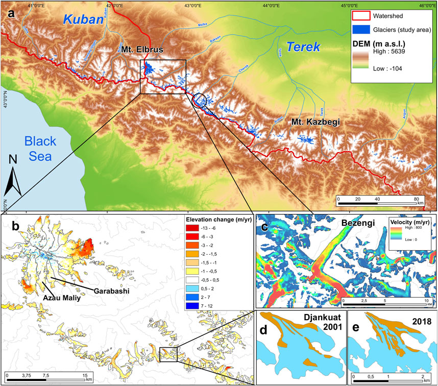
FIGURE 1. Study area. (A) Glaciers of the Terek and Kuban basins (northern macro slope of the Caucasus) are shown in blue (B) Changes in the surface elevation of glaciers in the central Greater Caucasus near Mt. Elbrus between 2000 and 2019 (Hugonnet et al., 2021). (C) Ice surface flow velocity in the region of the Bezengi glacier (Millan et al., 2022). (D) Debris cover of the Djankuat glacier as of the RGI inventory date (2001) and 2018 (E) (glacier outlines from Khromova et al. (2020)).

In our study, we focus on the Terek (655 glaciers, 638 km² total glacierized area) and Kuban (312 glaciers, 180 km² total glacierized area) river basins, which contain most of the glaciers of the northern slope of the Greater Caucasus (Figure 1). The count of 967 glaciers is according to RGI v.6.0 (typically 2000–2004) while the detailed inventory by Khromova et al. (2020) lists 1,309 glaciers in 2018. Many small glaciers, especially in the East Caucasus, were not included in the RGI data Tielidze et al. (2022). For the purposes of this study, this discrepancy does not play a major role, since we are interested in the relative change in ice volume. Glacier area reaches maximum at higher elevations in the Terek basin in comparison with the Kuban basin (Figure 2) because of the Kuban’s proximity to the Black Sea and, consequently, higher precipitation.

FIGURE 2

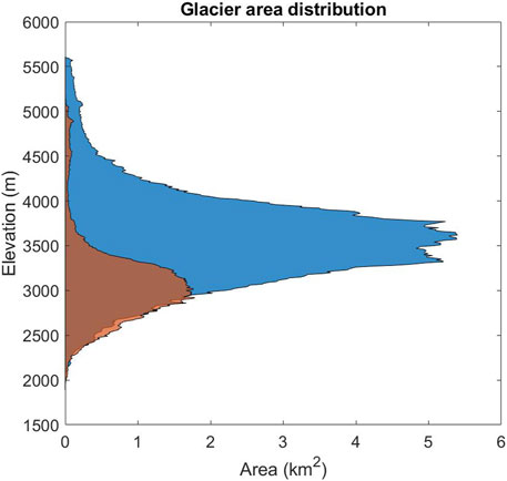
FIGURE 2. Elevation distribution of the glacier area in 2001/2004 for the Terek/Kuban basins.

2.2 Data

2.2.1 Glacier geometry

Glacier outlines for years 2001–2004 have been obtained from the RGI 6.0 inventory (RGI Consortium, 2017). Glaciers longer that 1 km, comprising 90% of total glacier area in the Terek basin and 78% in the Kuban basin, were considered. Hypsometry data from the SRTM DEM from 2000 (which agrees well with the glacier contours) were used. Glacier thickness was derived from an updated version of the data set published by Huss and Farinotti (2012, updated to RGI6.0). In general, these reconstructed ice thicknesses agree well with those from the radar sounding of glaciers on Mount Elbrus Kutuzov et al. (2019).

To represent glacier geometry in the model, the method of ‘elevation-band flowlines’ (Huss and Hock, 2015) was used. The elevation range of each glacier was divided into 10 m bands. Glacier characteristics such as area, slope, thickness, width and length were calculated for each elevation band. The flowlines obtained this way have irregular spacing dependent on the slope. For GloGEMflow, all glacier characteristics were interpolated along the irregular flowline linearly to a regular grid with a target resolution dependant on glacier length.

2.2.2 Climate forcing

The mass balance module of GloGEM was forced by 2 m temperature and precipitation data of the European Centre for Medium-Range Weather Forecasts Interim re-analysis (ERA-5) (Hersbach et al., 2019) for 1979–2020. For the future simulations until 2,100, simulations from 13 CMIP6 GCMs for five Shared Socioeconomic Pathways (SSP) (Eyring et al., 2016) were used: SSP1-1.9, SSP1-2.6 (low), SSP2-4.5 (medium), SSP3-7.0, SSP5-8.5 (most agressive), where the first digit denotes the SSP narrative, and the next two digits denote radiative forcing. The lowest forcing SSP1-1.9 leads to a likely increase of global temperature by no more than 1.5° relative to the pre-industrial conditions (O’Neill et al., 2016). All used datasets have monthly resolution. The consistency between the past climate data and future climate scenarios from CMIP6 was reached using de-biasing procedure (Huss and Hock, 2015). For that, we compared the mean monthly temperature and precipitation during the period 1980–2010 and calculated additive monthly biases for temperature and multiplicative monthly biases for precipitation. For the climate projections, these biases, assumed to remain constant in time, are superimposed on the closest GCM grid cell to ensure alignment between the datasets. Moreover, we undertake additional adjustments to the GCM air temperature data to account for differences in interannual variability that exist between the re-analysis and GCM time series. For each of the 12 months, we determine the standard deviation of temperatures over the period from 1980 to 2010 for both the re-analysis data and the GCM series. The variability bias in temperature, expressed as a ratio, is then calculated, and used to correct the future temperature timeseries. For more details, we refer the reader to Huss and Hock (2015).

2.2.3 Debris cover

Debris cover was manually mapped for the study area using satellite imagery from 2001 to calibrate the debris-cover module and from 2018 to validate the debris-cover evolution based on debris-cover area change (Figure 3). Glaciers longer that 1 km were considered. They comprise 90% of the total glacier area in the Terek basin and 78% in the Kuban basin. Satellite images from Landsat 7 ETM+ and Sentinel-2 were used to derive the outlines of the debris cover. According to our mapping, the total debris-cover area in the Terek and the Kuban basins expanded from 78 km² in 2001 (64 km² in Terek, 14 km² in Kuban) to 101.7 km² in 2018 (86.4 km² in Terek, 15.3 km² in Kuban). On average the debris-covered glaciers had 10% of their area covered by debris material in 2001 and 15.5% in 2018.

FIGURE 3

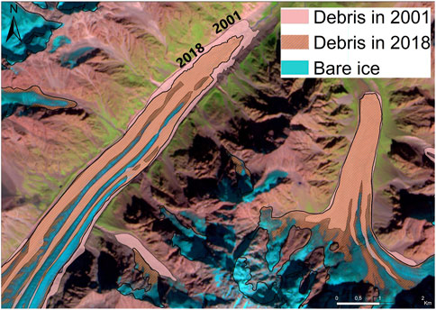
FIGURE 3. Examples of manual mapping of the supra-glacial debris cover. 2001 and 2018 dates corresponding glacier outlines. The Sentinel-2 image from 21 September 2020 is shown in the background.

No supraglacial ponds were detected probably because the strongly crevassed glacier surface allowed meltwater to filter away efficiently. Ice cliffs are rare and were present on several largest glaciers (e.g., Bezengi) probably because most glaciers are small and do not have long debris-covered snouts.

The database of debris-cover thickness by Rounce et al. (2021) was used for model calibration. Mean debris cover thickness was for each glacier based on the raster data from Rounce et al. (2021). Since this study does not account for the melt-enhancing effect of thin debris, raster cells with debris cover thickness in excess of 5 cm were considered.

For Djankuat glacier, on-site debris thickness measurements were accessible as documented by Popovnin et al. (2015), and these measurements exhibit substantial disparities when compared to the estimates by Rounce et al. (2021). Notably, the debris thickness values provided by Rounce et al. (2021) do not surpass 30 cm in the year 2008, whereas Popovnin et al. (2015) reported a maximum measured debris thickness of 260 cm in 2010. However, a comprehensive assessment of the uncertainties remains challenging due issues of comparability.

Specifically, Rounce et al. (2021) conducted a full range of calculations for debris cover thickness for glaciers exceeding an area of 2 km². Contrastingly, the available field measurements pertain only to the Djankuat glacier, which is inaccurately classified in the RGI as a glacier with an area smaller than 2 km². Consequently, for such glaciers, Rounce et al. (2021) relied on extrapolation methods. The result for Djankuat is thus uncertain and differences to in situ observations are difficult to be interpreted.

2.3 Model

2.3.1 GloGEMflow architecture

GloGEMflow (Zekollari et al., 2019) is a glacier model that uses the continuity equation in order to simulate the glacier evolution along the central flowlines. The mass balance is calculated following the positive degree-day approach and takes into account melt water refreezing. Ice deformation is calculated from the shallow-ice approximation (Hutter, 1983). In this study, GloGEMflow was equipped with a module for the debris-cover dynamics (see Section “Debris evolution module”).

The model initialization (left panel in Figure 4) serves to provide an internally consistent glacier geometry, its dynamics, the SMB and the debris cover. It comprises a calibration of the SMB module, ice flow module (the rheology parameter and a SMB offset) and debris cover module (debris expansion and deposition parameters) to generate an initial steady-state geometry (refer to Zekollari et al. (2019) for more details about calibration of GloGEMflow without debris).

FIGURE 4

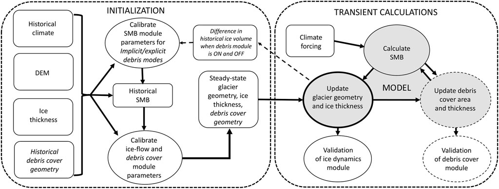
FIGURE 4. GloGEMflow architecture and link to the debris module. The calibration procedure is depicted in Figure 10. Here, the inner square blocks denote the input data needed for the computational blocks denoted by circles. The inner blocks denoted by dashed lines are the blocks that have been added to GloGEMflow to model the evolution of the debris cover. Shaded blocks illustrate the core of the model which consists of three modules: SMB, glacier dynamics and debris cover. Glacier dynamics module described in Zekollari et al. (2019) is denoted by a circle with a thick solid line.

This equilibrated state serves as a starting point for transient forward simulations (right panel in Figure 4). The model’s modules interact to model glacier evolution under changing climatic conditions. Firstly, SMB is calculated based on monthly meteorological forcing to compute specific mass balance for elevation bins of 10 m across a glacier. Secondly, SMB is adapted to account for debris cover, depending on its fractional area and thickness which are calculated from the debris cover module. Thirdly, the ice dynamics module computes the transport of ice and debris, and updates their distribution through time.

2.3.2 Mass balance

The SMB for the period of 1980–2,100 is computed based on meteorological data representing the processes of snow accumulation, snow and ice melt used a temperature-index approach, and refreezing of meltwater in snow and firn (Huss and Hock, 2015). The mass-balance module is calibrated for each individual glacier by varying the precipitation correction factor and the degree-day factors for snow and ice in order to match the glacier-specific geodetic mass balance over the period of 2000–2019 (Hugonnet et al., 2021) (Section “Calibration”).

We generate two SMB datasets: one for simulations in which debris is explicitly accounted for (‘debris-loaded’ dataset), and one for which debris is implicitly accounted for (‘debris-free’ dataset) (Figure 5). For the simulations with the debris-cover module (explicit approach), the debris-cover effect is completely excluded from the SMB dataset during the calibration process (Section “Calibration”). This allows us to isolate the influence of the debris flow module. For the simulations without the debris-cover module (implicit debris-cover approach), although the glacier evolves in a bare-ice mode, all the effects influencing the SMB including debris cover are inherent to the SMB due to the calibration of mass-balance module based on real mass-loss data.

FIGURE 5

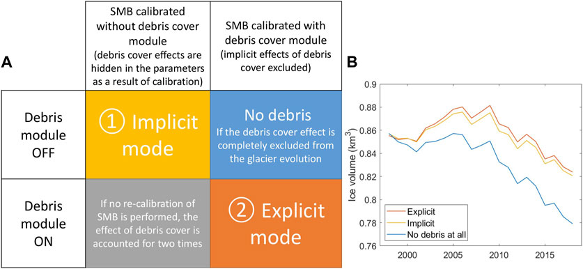
FIGURE 5. (A) Explicit and implicit modes of accounting for debris cover in the model. (B) Ice volume evolution of glacier Azau Maliy (RGI60-12.00168), where debris cover is treated explicitly (orange) and implicitly (yellow), and what happens if debris cover is completely excluded from the model (blue) (right panel).

2.3.3 Ice flow model

The GloGEMflow module is elaborately described in Zekollari et al. (2019). It considers glacier movement along a single flowline, i.e., glacier characteristics averaged over elevation bins are used as input data. It is based on mass-conservation and the rheological dependency of glacier velocity on stress:

$\left\{\begin{array}{c}\partial H/\partial t=-\nabla \left(\bar{u}H\right)+b\hfill \\ \bar{u}=2A/\left(n+2\right){\tau }^{n}H\hfill \\ \tau =-\rho gH\partial s/\partial x\hfill \end{array}\right.(1)$

where H (m) is the glacier thickness, $\bar{u}$ (m a⁻¹) is vertically averaged velocity, $\nabla (\bar{u}H)$ is the local ice flux divergence, b is the surface mass balance (m w. e. a⁻¹), A is the deformation-sliding factor (Pa⁻³a⁻¹), τ (Pa) is the driving stress, n - Glen’s flow law exponent, $\frac{\partial s}{\partial x}$ - surface slope. Similar to Zekollari et al. (2019), we combine the effects of basal sliding and ice deformation into a single variable since both of them are linked to surface slope and ice thickness, and thus have very similar spatial patterns (Zekollari et al., 2013).

2.3.4 Debris cover evolution module

The debris evolution module was adopted from Verhaegen et al. (2020) who simulated the evolution of the Djankuat glacier along its flow line, thereby accounting for evolving debris cover. This approach was based on the debris model of Anderson and Anderson (2016) where debris-cover input was generated at a single point by means of hillslope erosion. In order to apply the debris cover model to a regional study, we seamlessly integrated this subroutine into GloGEMflow. This integration process necessitated several steps: 1) enhancing its computational efficiency to ensure faster processing, 2) adopting the premise that debris deposition occurs primarily in the upper accumulation zones of each glacier, and 3) integrating a calibration approach to fine-tune the evolution of the debris cover.

2.3.4.1 Debris cover thickness change in time

The debris thickness changes in each node along the flowline due to 1) meltout of englacial debris, 2) downstream advection of supraglacial debris, 3) input of the material from the debris deposition point (in upper accumulation zone) or output to the glacier foreground, calculated as follows (Verhaegen et al., 2020):

$\frac{\partial h_{\mathit{debris}}}{\partial t}=\underset{\left(1\right)}{\underbrace{-\frac{c_{\mathit{debris}}\mathit{min}\left(0,b_a\right)}{\left(1-{\varphi }_{\mathit{debris}}\right){\rho }_{\mathit{debris}}}}}\underset{\left(2\right)}{\underbrace{-\frac{\partial \left(u_{\mathit{surf}}{h}_{\mathit{debris}}\right)}{\partial x}}}+\underset{\left(3\right)}{\underbrace{I_{\mathit{debris}}}}(2)$

Here, h_debris m) is the debris thickness, t a) is time, 1) c_debris is the englacial debris concentration, ϕ_debris is the debris porosity, ρ_debris is the debris rock density, b_a is the annual surface mass balance, 2) u_surf is the surface velocity, 3) I_debris is the input or output of debris (Table 1). As such, our model has two sources of debris cover described in Equation 2: deposition at the source point and emergence in the ablation area due to meltout. The terms ‘deposition’ and ‘emergence’ will be used hereinafter to distinguish between them.

TABLE 1

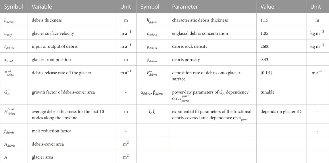
TABLE 1. Variables and parameters used in the debris cover module.

Figure 6 illustrates the glacier velocity pattern (panel c) which shapes the debris thickness profile (panel b). In the mid ablation zone where the surface velocity reaches its maximum, debris thickness reaches its minimum since the material is quickly advected downstream. The thickest layer of supraglacial debris is accumulated in the frontal zone where the velocity is the lowest. That is consistent with the result of Anderson and Anderson (2016) who show that the debris thickness is the smallest where the ice velocity is the highest and vice versa.

FIGURE 6

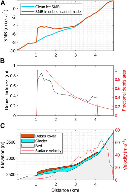
FIGURE 6. (A) Mass-balance profile with the debris-cover-corrected mass balance (orange), using the example of the Shkhelda Glacier (RGI60-12.00849) in the Central Caucasus in 2019. Blue line represent uncorrected mass balance for ’pure-ice’ glacier. (B) The fractional debris covered area and debris thickness on the Shkhelda Glacier in 2019 which produces the reverted mass-balance gradient shown in (A). (C) Corresponding glacier geometry and velocity (the debris cover thickness is scaled-up by a factor of 50 for visibility on panel c).

Since Equation 2 is an advection problem, the timestep should satisfy the Courant–Friedrichs–Lewy (CFL) condition. This means that the distance that the debris cover travels during one timestep must be lower than the distance between mesh elements. However the debris transfer along the glacier is described by the term 2), which depends on the glacier surface velocity. Therefore the timestep for the numerical implementation of the debris-cover advection equation was chosen to be the same as the timestep for the ice-dynamics module. It is calculated according to a CFL-type criterion (following the original GloGEMflow approach, Zekollari et al. (2019)) and depends on the spatial resolution which is different for each glacier (resulting in, for example, about 0.1 years for the Djankuat glacier). The spatial resolution is chosen in accordance with the overall size of each individual glacier, ensuring that every glacier is covered by 100 nodes along the elevation-band flowline. Values ϕ_debris, ρ_debris and c_debris were measured on the Djankuat glacier by Bozhinskiy et al. (1986) and assumed to be constants for the whole study area: ϕ_debris = 0.43 and ρ_debris = 2,600 kg m⁻³, c_debris = 1.05 kg m⁻³. For the sensitivity experiments other values for c_debris are tested.

The debris is deposited at the source point near the top of the glacier at a rate of $F_{\mathit{debris}}^{\mathit{input}}$ m year⁻¹ and is deposited at the foreland at a rate of $F_{\mathit{debris}}^{\mathit{out}}$ m year⁻¹:

$F_{\mathit{debris}}^{\mathit{out}}=-h_{\mathit{debris}}\left(x_{\mathit{front}}\right)\cdot b\left(x_{\mathit{front}}\right).(3)$

Therefore, the input or output of debris component is calculated as follows:

$I_{\mathit{debris}}\left(x\right)=\left\{\begin{array}{c}{F}_{\mathit{debris}}^{\mathit{input}}\text{\hspace{0.17em}if\hspace{0.17em}}x=x_{\mathit{debris}}\hfill \\ -F_{\mathit{debris}}^{\mathit{out}}\text{\hspace{0.17em}if\hspace{0.17em}}x=x_{\mathit{front-1}}\hfill \\ F_{\mathit{debris}}^{\mathit{out}}\text{\hspace{0.17em}if\hspace{0.17em}}x=x_{\mathit{front}}\hfill \\ 0\text{\hspace{0.17em}else},\hfill \end{array}\right.(4)$

where x_debris is the distance to debris deposition location.

When c_debris is as small as the one proposed for the Djankuat glacier (Bozhinskiy et al., 1986; Verhaegen et al., 2020), the meltout component plays a negligible role compared to the deposition plus advection components. If the meltout is removed from the model, it will produce almost the same results, since the debris deposited in the accumulation area and advected to the ablation area emerge and modify the mass balance independently of the meltout component. Moreover, englacial debris concentration should depend on the debris deposition - the more debris is entrained in the accumulation area, the more debris is concentrated in the ice as it reaches the ablation area. This leads us to the suggestion that we could instead use a larger c_debris for the meltout, and turn off debris deposition, so meltout would be the only source of debris on the glacier. So experiments were conducted to assess the sensitivity of model predictions to ‘deposition-driven’ or ‘meltout-driven’ debris cover module. For this sensitivity analysis we implemented the following modification of Equation 2, where deposition of debris cover at the source point is turned off:

$\frac{\partial h_{\mathit{debris}}}{\partial t}=\underset{\left(1\right)}{\underbrace{-\frac{c_{\mathit{debris}}\mathit{min}\left(0,b_a\right)}{\left(1-{\varphi }_{\mathit{debris}}\right){\rho }_{\mathit{debris}}}}}\underset{\left(2\right)}{\underbrace{-\frac{\partial \left(u_{\mathit{surf}}{h}_{\mathit{debris}}\right)}{\partial x}}}+\underset{\left(3\right)}{\underbrace{F_{\mathit{debris}}^{\mathit{out}}}}(5)$

As such, there is no deposition component in debris cover influx, only debris cover emergence by meltout, which is controlled mainly by englacial concentration parameter.

2.3.4.2 Debris cover area change in time

The debris-cover shapefile produced for this study and a DEM from 2000 were used to extract the area distribution of the debris cover for each RGI glacier (RGI Consortium, 2017) for every elevation band. This data was loaded into the debris module and interpolated into GloGEMflow horizontal grid (Figure 7). The fraction of debris-covered area at the inventory date was calculated by dividing debris cover area by glacier area for each node along the flowline (distance between nodes is adjusted for each glacier, see Section “Debris evolution module”) (Figure 7). After that, the fractional area of the debris-covered ice at the inventory date is approximated by an exponential function (Figure 7) according to the equation:

$\frac{A_{\mathit{debris}}\left(x\right)}{A\left(x\right)}=\zeta e^{\left(x-x_{\mathit{front}}\right)\xi },(6)$

where x_front (m) is the glacier front position, A_debris(x) (m²)is debris-cover area at the distance x along the flowline, A(x) (m²) is glacier area at the distance x, and ζ and ξ are fitting parameters. Coefficients for the exponential fit were calculated for each RGI glacier separately. They were further used in order to adjust debris cover area distribution, as the glacier evolves throughout the simulations.

FIGURE 7

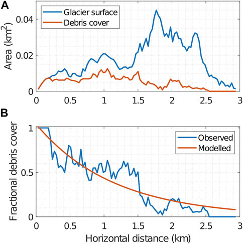
FIGURE 7. (A) Glacier area (blue) and debris-cover area (orange) distribution along the ’elevation-band flowline’ of the Djankuat glacier (RGI60-12.01132). (B) The fractional debris-covered area distribution along the flowline (blue) and exponential fit used to approximate it in the debris-cover module (orange). The horizontal axis represents distance along the flowline from the glacier terminus at 0 km.

The fraction of debris-covered ice for other years (which obviously does not exceed 1, Figure 6B) along the flowline is parameterized depending on the distance from the glacier front (x − x_front):

$\frac{A_{\mathit{debris}}\left(x\right)}{A\left(x\right)}=G_A\cdot \left(\zeta \cdot e^{\left(x-x_{\mathit{front}}\right)\cdot \xi }\right).(7)$

A_debris is debris-cover area, A is glacier area.

$G_A={\alpha }_{\mathit{debris}}{(H_{\mathit{debris}}^{\mathit{front}})}^{{\beta }_{\mathit{debris}}}$ is the debris cover area growth factor which is updated every model year. It means that the larger is the debris cover thickness in the frontal area $H_{\mathit{debris}}^{\mathit{front}}$, the larger is the fraction of debris coverage of the glacier, but its exponential distribution is always preserved.

The debris module integrated into the GloGEMflow model is constructed based on a set of assumptions. These assumptions, although not entirely accurate, were necessary due to the limited data availability and the need for computational efficiency. The key assumptions of the debris module are as follows.

• We assumed that all debris cover within the study area has a thickness greater than 5 cm. Consequently, the potential impact of ablation enhancement under thin debris cover was neglected. While this assumption may not hold true in all cases, it is worth noting that the Caucasus region is generally characterized by a prevalence of thick debris cover (Rounce et al., 2021). Furthermore, observations have indicated that areas with debris thinner than 5 cm are typically found near the accumulation zone and not associated with ice thinning (Huang et al., 2018).

• The debris rock density and porosity are assumed to be uniform throughout the study area and are set to the values measured at Djankuat Glacier.

• The englacial debris concentration is assumed to be constant for all glaciers.

2.3.5 Mass balance change due to debris cover

The surface mass balance of the debris-covered glacier is calculated by correcting the bare-ice melt by a function that depends on the debris thickness and the fractional debris-covered area. The sub-debris melt is assumed to decrease exponentially with the increase of the debris cover thickness (Winter-Billington et al., 2020). Therefore the melt reduction factor f_debris (a term introduced in Verhaegen et al. (2020)) is calculated depending on the debris-cover thickness (Verhaegen et al., 2020):

$f_{\mathit{debris}}=e^{\frac{-h_{\mathit{debris}}}{h_{\mathit{debris}}^{*}}}(8)$

where $h_{\mathit{debris}}^{*}$ is the characteristic debris-cover thickness. It is the thickness at which actual melt under debris reduces to e⁻¹ or 37% of the bare-ice melt.

Bare-ice ablation (b_input), which is calculated using degree-day approach and serves as the input to the dynamic module of GloGEMflow, is adjusted according to the characteristics of the modelled debris cover - thickness and fractional area. SMB of debris-covered ice is calculated for each elevation band along the flowline as follows:

$b_{\mathit{debris}}=b_{\mathit{input}}\cdot \frac{A_{\mathit{debris}}}{A}\cdot f_{\mathit{debris}}$

SMB of debris-free ice is equal to:

$b_{\mathit{debrisfree}}=b_{\mathit{input}}\left(1-\frac{A_{\mathit{debris}}}{A}\right)$

The resulting SMB b consists of the following components:

$b=b_{\mathit{debris}}+b_{\mathit{debrisfree}}$

As a result, the model produces a reversed mass-balance gradient (where SMB decreases with increasing elevation) in the ablation area of the debris-covered glacier (Figure 6A) based on modelled debris thickness and fractional area (Figure 6B), which are mostly controlled by the glacier dynamics (Figure 6C).

2.4 Calibration

Calibration of all three modules of the model was performed on the glacier-specific scale.

2.4.1 Mass balance module calibration

The GloGEMflow mass-balance module calibrates three parameters to match glacier-specific geodetic mass balance between 2000 and 2019 provided by Hugonnet et al. (2021): i) precipitation correction coefficient, which performs the function of adjusting climatic data to specific glacier features (local topographic effects, rain shadow, etc.); ii) degree-day factors (DDF), which translate the number of days with positive temperature into melt of snow or ice; iii) temperature correction for inaccuracies caused by the insufficient spatial resolution of climatic data. The GloGEMflow mass-balance module uses a three-step calibration procedure: first, the precipitation correction parameter is calibrated; then, if deviations from the mass-balance data remain large, the DDF parameter is calibrated; if the second step does not give a good enough result, the temperature correction parameter is systematically shifted. For more details, refer to Huss and Hock (2015).

In order to assess the debris-cover effect on the glacier evolution, two mass-balance data sets were created: a ‘debris-free’ and a ‘debris-loaded’ dataset (Figure 5). For the “debris-free” mass-balance data set, the parameters described above were tuned presuming the glacier to be debris-free in the model. Since the DDF parameter can be interpreted as the reaction of the glacier on the temperature change, in this case the effect of debris cover on glacier evolution is taken into account implicitly. The second mass-balance data set for ‘debris-loaded’ glacier representation was created by re-calibrating the mass-balance model using the explicit debris-cover formulation.

The two mass-balance datasets were obtained by the following method. The calibrated dynamic model was forced by ERA5 reanalysis data until 2019. The difference between the volume change rates between 2000 and 2019 with and without debris cover for each glacier were quantified (Figure 4). This mass-balance gap was taken into account for the re-calibration of the mass-balance module parameters.

The ice mass losses in the 2000–2019 period resulting from the debris-free (implicit) and debris-loaded (explicit) simulations were similar. However, the spatial patterns of mass-balance distribution were different (Figure 6). This affects glacier characteristics such as surface velocity (Figure 8), terminus location, shape of the glacier profile, and thinning rate (Figure 9). Since debris cover increases value of mass balance in the ablation zone, mass balance in the ‘debris-loaded’ data set is generally slightly more negative than in the ‘debris-free’ data set to compensate for the debris-cover effect.

FIGURE 8

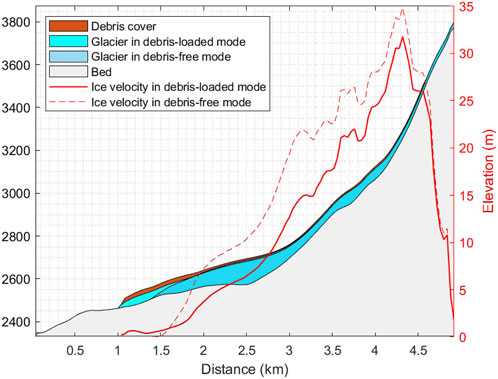
FIGURE 8. Vertically averaged velocity and the profile of the Bashkara glacier (RGI60-12.00849) in 2019 in debris-free and debris-loaded mode. Volume of the glacier is equal to 0,15 km³ in both debris-free and debris-loaded mode, since in both cases the mass balance was calibrated to meet the data from Hugonnet et al. (2021). However, the shape of the glacier is different: debris-covered glacier lost volume mostly by downwasting, while debris-free glacier - by backwasting.

FIGURE 9

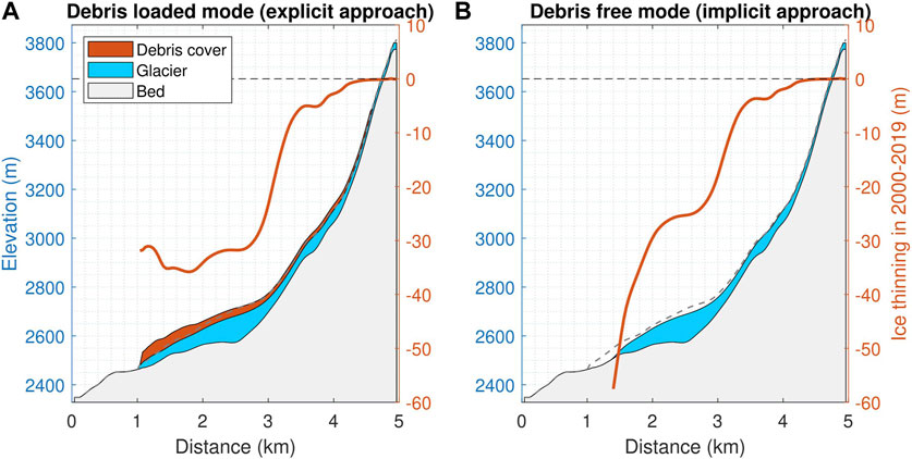
FIGURE 9. Thinning rate of the Bashkara glacier between 2000 and 2019 when accounting for debris cover explicitly (A) and implicitly (B). The shaded area indicates the zone of maximum thinning identified by Anderson et al. (2021). Debris-cover thickness is magnified a hundredfold for clarity.

2.4.2 Ice flow module calibration

The calibration of the GloGEMflow model while accounting for the newly-introduced debris cover module consisted of three stages (Figure 10).

I. For each glacier the rheological-sliding parameter was calibrated to fit the RGI glacier geometry in debris-free mode at the inventory date.

II. The debris cover module was calibrated to fit the observed debris area and thickness in 2001/2004.

III. For each glacier, the rheological-sliding parameter was re-calibrated to fit RGI glacier geometry with imposed debris cover at the inventory date.

FIGURE 10

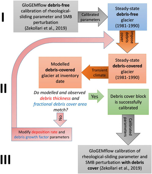
FIGURE 10. Three steps of the GloGEMflow model calibration (see the subsection ”Ice flow model” in the ”Calibration” section for the description), accounting for the newly introduced debris cover module. Step I and III consist of calibration of the rheological-sliding parameter of a glacier without (I) and with (III) evolving debris cover. Step II consists of calibration of the fractional area growth factor and debris deposition rate.

The GloGEMflow calibration procedure Zekollari et al. (2019) aimed to accurately reproduce glacier geometry from RGI. First, the model was initiated from ice-free conditions. It was forced by mass balance corresponding to the 1981–1990 climate until steady state was reached. Glacier then evolved between 1990 and the inventory date. The deformation-sliding factor A was calibrated to match glacier volume to the RGI data. SMB perturbations were imposed to match glacier length to the RGI data.

2.4.3 Debris cover module calibration

For each glacier featuring debris cover (139 glaciers in the Terek basin, 42 glaciers in the Kuban basin) three parameters were tuned: i) $F_{\mathit{debris}}^{\mathit{input}}$ - the input flux of debris from the deposition location; ii) parameters α_debris and iii) β_debris of power dependency of G_A (that determine growth of the fractional debris-covered area) from the frontal debris thickness

$G_A={\alpha }_{\mathit{debris}}{\left(H_{\mathit{debris}}^{\mathit{front}}\right)}^{{\beta }_{\mathit{debris}}}.(9)$

2.4.3.1 Calibration of the debris-covered fractional area growth factor

The goal of the calibration step II was to reduce the root-mean-square error (RMSE) for the parameters α_debris and β_debris to less than 0.01 when reproducing the fractional debris-covered area for all elevation bins where the debris cover is present. RMSE between the modelled fractional debris-covered area $(A_{\mathit{debris}}^{mod})$ and the observed fractional debris-covered area $(A_{\mathit{debris}}^{\mathit{obs}})$ is equal to

$RMSE=\sqrt{\frac{{\sum }_{i=1}^n{\left(A_{\mathit{debris,i}}^{\mathit{obs}}-A_{\mathit{debris,i}}^{mod}\right)}^2}{n}},$

where n is the amount of ice-covered points on the grid. The procedure for calibrating the parameters of the debris module is described in the Appendix. They lie within the ranges α_debris ∈ [0.67, 4.33] with the mean value of 1.75, and β_debris ∈ [0.2, 1.15] with the mean value of 0.59. We assume that the dependency between the fractional debris-covered area growth and the modelled mean debris thickness at the glacier front will be the same in the future as for the time before the inventory date.

Following step II, glaciers with debris cover and the same rheology parameter as in step I (debris-free calibration) exhibited a slight increase in size at the inventory date (Fig. S1) due to the introduction of debris cover. Consequently, step III was necessary to re-calibrate the rheological parameter and align it with the inventory geometry. The debris cover growth factor dependency values, specific to each glacier, were carried over from step II to the calibration process in step III.

2.4.3.2 Debris deposition rate calibration

The accumulation of debris cover in the source area was determined by the deposition-rate parameter, denoted as $F_{\mathit{debris}}^{in}$. This parameter directly influences the debris thickness in the model being a component of the I_debris Equation 2. The rate of debris deposition onto the glacier was calibrated using the modeled values for debris thickness presented in (Rounce et al., 2021). For glaciers smaller than 2 km², Rounce et al. (2021) calculated debris cover thickness by extrapolating parameters obtained for larger glaciers (more than 2 km², there are 65 such glaciers in the Terek basin with total area of 410 km² and 23 glaciers in the Kuban basin with total area of 71 km²). However, the measured debris cover thickness on the Djankuat glacier (whose area was wrongly defined in RGI as less than 2 km²) (Popovnin et al., 2015), was not realistically represented in Rounce et al. (2021). Therefore, we chose two calibration strategies.

1. Calibrate deposition rate for all glaciers using the debris thickness from Rounce et al. (2021);

2. Calibrate deposition rate for glaciers larger than 2 km² according to Rounce et al. (2021), and for glaciers less than 2 km² using the same deposition rate value as for the Djankuat Glacier, obtained from the observational data.For the Djankuat glacier, the debris deposition rate value $F_{\mathit{debris}}^{in}=0.55$ m a⁻¹ was calibrated by a trial and error procedure and was the same as in Verhaegen et al. (2020). For the glaciers, which are meant to be calibrated using debris thickness values from Rounce et al. (2021), to be consistent, we use the same calibration method for $F_{\mathit{debris}}^{in}$ as was used in GloGEMflow (Zekollari et al., 2019) for ice-flow module calibration (See Appendix for the details). The goal of the calibration procedure was to meet the glacier-wide mean debris-cover thickness in the year 2008, which was chosen as a reference year by Rounce et al. (2021). By iteratively adjusting the deposition rate based on the model’s accuracy in estimating the debris cover thickness, the process converges to the reference thickness within four to five iterations. Calibrated values of the deposition rate were allowed to vary between 0.1 and 1 m per year.

We assessed the performance of different calibration methods by evaluating their ability to accurately represent the total accumulated debris cover area by 2018. Based on our evaluation, we selected the second calibration scheme due to its superior performance, as the implementation of the first calibration scheme resulted in an underestimation of the debris cover area.

3 Results

3.1 Validation of the new debris cover module

For validation of the debris cover module we used the area of debris cover change on each glacier between 2001 and 2018. To achieve that, we mapped the debris cover manually from Landsat 7 ETM+ and Sentinel-2 imagery from the year 2018. The debris-cover area change accumulated in the transient simulation from 2001 by 2018 was then compared to the observed for each individual glacier (203 points on Figure 11). The modelled debris-cover area change is well correlated to the observed (R² = 0.66, RMSE = 0.18 km²) (Figure 11).

FIGURE 11

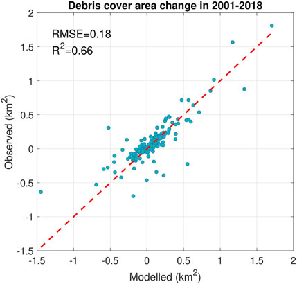
FIGURE 11. Observed vs. modelled debris-cover area change in 2001-2018 for the glaciers in Terek and Kuban basins.

3.2 Ice velocity

The presence of debris cover significantly influences the surface profile and ice-velocity gradient of glaciers (Figure 8). Modelled debris-covered glaciers often exhibit a characteristic concave shape of the velocity gradient, which was not observed at the same glaciers modelled without the debris cover module. This distinction was due to the specific characteristics of debris-covered glaciers, where those with elongated flat tongues tend to experience volume loss through downwasting (Nuimura et al., 2012). As a consequence, these glaciers exhibited a thinner ice profile with a relatively stable terminus position. On the other hand, debris-free glaciers predominantly undergo volume loss through backwasting, leading to quicker terminus retreat (as discussed in the “Ice thinning” section). Consequently, when debris was incorporated into the glacier model, the glacier became longer and thinner in the mid-ablation zone by 2019 compared to the same glacier modelled without the debris cover module, while maintaining the same ice volume in 2019.

As a result, in the mid-ablation zone, the explicit modelling of debris cover led to lower glacier velocities due to the thinner ice profile and reduced surface slope. On average, when the debris cover was explicitly modelled, the mean velocity is 6.5% lower in the Kuban basin and 2% lower in the Terek basin compared to the implicit approach.

3.3 Ice thinning

Although glaciers lose similar ice volume in 2000–2019 in ‘debris-loaded’ and ‘debris-free’ cases, a distinct thinning pattern emerged when debris was explicitly modeled during this period. Specifically, the ice initially thinned in the mid-ablation zone, known as the ‘zone of maximum thinning’ (Anderson et al., 2021) while glacier length remained almost unchanged over this time period. Conversely, this pattern was not observed in glaciers where debris cover module was not employed. Figure 9 shows that, under the debris-loaded mode relative to the debris-free mode, thinning was lower within the first 1–2 km upstream from the zero x coordinate (area-averaged ice thinning of 40 m under debris-free mode and only 34 m under debris-loaded mode), higher in mid-ablation zone between 2 and 3 km (area-averaged ice thinning of 24 m under debris-free mode and 30 m under debris-loaded mode), and approximately equal from 3–5 km (around 4 m of ice thinning). According to Benn et al. (2012) and Anderson et al. (2021), amplified thinning in the middle zone of the glacier is controlled by debris-perturbed driving stress and vice versa. When most of the mass loss occurs in the mid zone, the surface gradient decreases, which lowers the driving stress and glacier velocity at the front. Therefore, dynamic ice inflow into frontal area decreases, and the glacier tongue melts away (Ferguson and Vieli, 2021). These results were consistent with the observed thickness changes in the Caucasus (Hugonnet et al., 2021) as well as with observations and modelling results from other regions (Hambrey et al., 2008; Banerjee and Shankar, 2013; Brun et al., 2019).

3.4 Debris cover thickness change

We calculated area-averaged debris cover thickness for each combination of climate model and scenario (Figures 12A,B). Debris cover thickness change show quite similar trends in the Terek and Kuban basins, although the uncertainty associated with the Terek basin depending on the climate scenario is larger (Figures 12A,B). From an initial area-averaged value of approximately 0.4 m in the Terek basin and 0.5 m in the Kuban basin in 2020, the mean regional debris cover thickness grows until 2040, and then generally exhibits a decreasing trend under all climate scenarios until 2,100. The extent of the decline in debris cover thickness is larger in warmer climate scenarios. Under all climate scenarios except SSP5-8.5 mean debris cover thickness is projected to remain above 7 cm on average until 2,100 (Figures 12A,B).

FIGURE 12

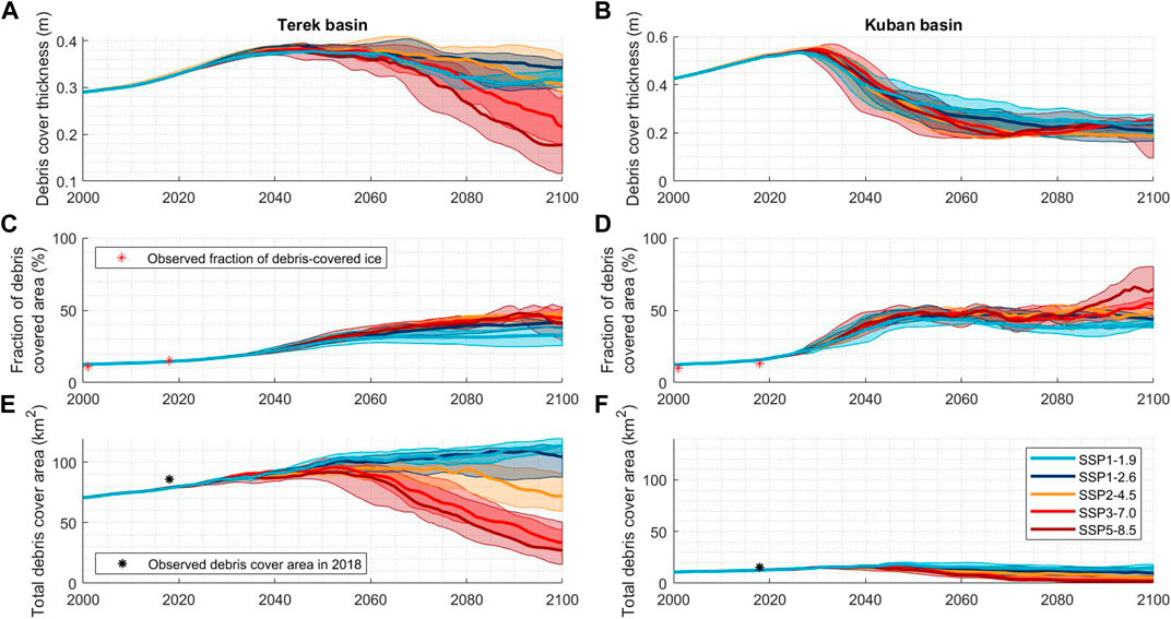
FIGURE 12. Debris cover thickness [(A) - Terek, (B) - Kuban] and area change [fractional area: (C) - for the Terek basin, (D) - for the Kuban basin; total area: (E) - Terek, (F) - Kuban] under different future climate forcing scenarios. Thick lines correspond to a median value for different climate model forcings within each SSP scenario. Here, the lines for debris thickness are smoothed for clarity. Shadowed areas represent the range between minimum and maximum values for each scenario.

3.5 Debris cover area change

Our results showed that fractional debris coverage of glaciers in the Terek basin exhibited a nearly linear increase from 15% to 25.6% ± 2.4% between 2020 and 2050 under all climate scenarios. In the Kuban catchment, fractional debris coverage increased at a faster rate, reaching 40% ± 8% by 2050 (average for all scenarios). Beyond 2050, the fraction of debris-covered ice either stabilized for the less aggressive scenarios (SSP1-1.9 for the Terek basin and SSP1-1.9, 1–2.6, 2–4.5 for the Kuban basin) or continued to increase for other scenarios (Figures 12C,D). Notably, fractional debris cover was higher in both basins under the warmer climate scenarios after 2050. By 2,100, it ranged from 25% for the SSP1-1.9 to 50% for the SSP5-8.5 in the Terek basin, and from 25% to (with high uncertainty since for the SSP5-8.5 almost all ice left is the Kyukyurtlyu glacier) 80% in the Kuban basin. The projected total debris cover area in the Terek basin will continue to increase almost linearly until 2025 under all climate scenarios. After 2050, the projected debris cover area will become more sensitive to both climate scenarios and the choice of GCMs in both basins. Overall, larger total debris cover areas were predicted for the moderate scenarios in both basins. They may increase under the least aggressive climate scenarios (SSP1-1.9 and SSP1-2.6) and decrease under the warmer scenarios. In the future, the total debris cover in the Kuban basin could completely disappear under the SSP5-8.5 scenario, while reaching a maximum of 17 km² under the SSP1-1.9 scenario (Figure 12F). For the Terek basin, the projected values ranged from 1.9 km² to 121 km². Notably, the total debris cover area in both basins was highest in 2,100 for scenarios with the weakest warming.

3.6 Ice volume change

Between 2015 and 2,100 the glaciers in the Terek basin were projected to lose between 43% ± 27% (SSP1-1.9, median and inter-quartile range) and 98% ± 1% (SSP5-8.5) of their 2015 total ice volume, independently of whether the debris-cover module is activated or not (Figure 13, S2). For the Kuban basin, the respective ice-volume loss ranged from 63% ± 36% to 99% ± 2% (Figure 13), with the difference between implicit and explicit debris-cover formulation also being negligible for all scenarios except SSP1-1.9 by 2,100.

FIGURE 13

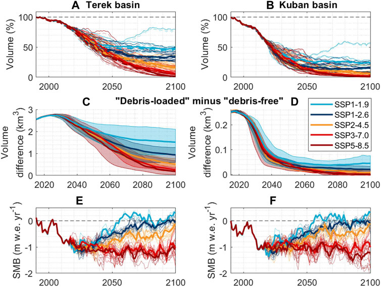
FIGURE 13. Glacier volume in the Terek (A,C) and the Kuban (B,D) river basins [(A,B) - relative to 1990, solid line - in debris-loaded mode, dashed line - in debris-free mode] and SMB evolution in the Terek (E) and the Kuban (F) basin in 1990-2100. Thick lines represents median of the results for all GCMs for each scenario. Thin lines represent the results for each GCM.

Until 2035, glaciers of both basins lose ice at a constant rate if median values are considered. However, the rate of ice loss was almost twice as high in the Kuban basin compared to the Terek basin (Figure 13). Linear ice volume loss was followed by gradient flattening projected for different times depending on the basin and climate scenario (Supplementary Table S1). In general, the decrease of ice volume loss rate started earlier for scenarios with less warming, and earlier for the Kuban basin compared to the Terek basin. Ice volume stabilized in 2040 under SSP1-1.9 scenario. Moreover, SSP1-1.9 allowed for a slight increase in ice volume after 2050, and one GCM (CAMS-CSM1-0) predicted glacier advance after 2050 almost reaching the same extent in 2080 as in 2015.

The ice loss rate varied greatly between the basins and between the first and the second half of the century. For example, in 2000–2050, glaciers of the Terek basin lost ice at a rate between 0.34 km³ a⁻¹ (SSP1-1.9) to 0.42 km³ a⁻¹ (SSP5-8.5) if the debris cover was modelled explicitly. If the debris-cover mode was deactivated, ice loss was 1% higher. In 2050–2,100, when glaciers retreat to higher altitudes, the model showed ice-volume gain at a rate 0.028 km³ a⁻¹ when forced by SSP1-1.9 scenario (the gain is larger, 0.032 km³ a⁻¹, if the debris cover evolution is not considered), and ice loss rate up to 0.24 km³ a⁻¹ for the SSP5-8.5 scenario (0.22 km³ a⁻¹ in debris-free mode). Thus, in the first half of the century when the mass balance is strongly negative, the debris cover slightly slowed down the modelled ice-loss rate. On the contrary, when glaciers stabilize at the second half of the century, glaciers with the explicitly-modelled debris exhibited higher ice losses than in the implicit-debris mode. The difference between glacier volume in debris-loaded (explicit) and debris-free (implicit) debris modes may thus be eliminated by 2,100.

There is a large variability between simulations forced by different GCM even within a single SSP scenario. For example, under SSP1-1.9, GloGEMflow forced by the climate model EC-Earth3-Veg simulated constant decline of ice volume which was larger under the debris-free mode after 2019 (Supplementary Figure S2). On the contrary, GloGEMflow forced by CAMS-CSM1-0 climate model simulated change from mass loss to mass gain around 2050 while the difference made by the debris-cover module application reached its maximum of 2.5% around 2040 when the volume loss rate started to decrease. The debris-cover effect (represented by the shaded area in Supplementary Figure S2) then declined until 2080 when the loss produced in the debris-loaded mode became 1.7% larger than in the bare-ice mode (Supplementary Figure S2).

3.7 Glacier length change

The model predicted that on average, lengths of the debris-covered glaciers will decrease slowly (i.e., one grid cell per several years) until 2035 (this year for an individual glacier depends on its size: the larger the glacier, the later the acceleration of retreat occurs; Figure 15). This gradual decline can be attributed to a combination of factors, including the presence of debris cover which insulates ice reducing the rate of retreat. As a result, the glaciers maintained a relatively stable front position during this initial phase. Following the substantial glacier thinning, the model predicts much more rapid retreat of glacier fronts in a step-wise manner, often accompanied by detachment of large dead ice areas from the main glacier bodies. When glaciers were modelled in the debris-free mode, rapid glacier front retreat started earlier and was more gradual. This disparity can be attributed to the absence of debris cover, which allows for a more direct interaction between the ice and the surrounding environment. Without the insulating effect of debris, glaciers experienced faster melting rates and faster frontal retreat.

3.8 Ice extent change

Under the most extreme SSP5-8.5 scenario, glaciers were preserved mostly on the Mount Elbrus above 4,000 m a.s.l. In the Terek basin, 84% of the ice left by 2,100 (0.42 km³) was located on the Elbrus (Figure 14A). Under the SSP1-1.9 scenario, the share of the Elbrus glaciers in the total ice area in 2,100 is 30% only. In the Kuban basin, under the SSP5-8.5 scenario, 98% of the remaining ice (0.015 km³) is concentrated on the Elbrus (Figure 14B). Maps in Supplementary Figure S3 show an example of ice geometry in 2,100 in the central part of the Terek basin under the SSP1-2.6 and SSP5-8.5 scenarios. Under SSP5-8.5, almost no ice is left in the Main Caucasian Ridge. Under SSP1-2.6, large glaciers retreat and become fragmented while small glaciers disappear. However, at higher elevations thick ice (e.g., more than 300 m in case of the Karaugom glacier) may be preserved.

FIGURE 14

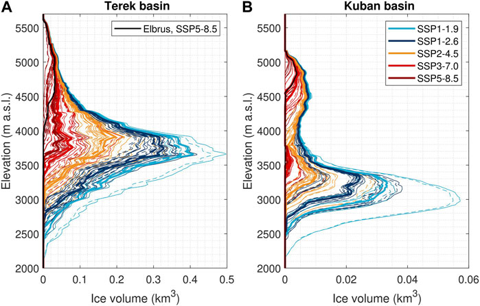
FIGURE 14. Distribution of ice volume across elevation bands in 2100 in the (A) Terek and (B) Kuban basins under different future climate scenarios, in ’debris-covered mode’. Each line corresponds to a combination of the climate model and the SSP scenario. Black line denotes ice volume on Elbrus.

3.9 Mass balance

Under all scenarios, in the first half of the century glaciers were predicted to retreat to higher elevations, where lower temperatures lead to the less negative mass balance. With reference to the median values (of a range of different climate-model realisations), future mass-balance evolution under the low-warming SSP1-1.9 is characterised by negative mass balances before 2050, while in the second half of the century the mass balance periodically turns to positive values (Figures 13E,F). Specifically, Figures 13E,F shows that positive mass balances are predicted for the Terek basin from approximately 2055–2075, fluctuate around zero afterwards and become positive after 2087. A similar pattern is observed in the Kuban basin. Furthermore, positive values were predicted in both basins under the SSP1-2.6 scenario for multiple glaciers with zero mean value after 1987.

For the SSP1-2.6 scenario, the mass balance trend changes sign in 2025. Under the SSP2-4.5 scenario, mass balances increases for all glaciers in both basins consistently from approximately 2035. Under SSP3-7.0, mass balances trend upward over the final 10–15 years of the simulations in both basins, and predicted mass balances also increase in the Terek basin in the last 10 years of the simulations made for the SSP5-8.5 scenario. Under the most extreme SSP3-7.0 and SSP5-8.5 scenarios, mass balance declines until 2050. After that glaciers quickly retreat to higher elevations, and the median mass balances fluctuate between −1.5 and 1 m w. e.a⁻¹.

3.10 Dead ice areas change in time

Dead ice areas are characterized by the presence of stagnant ice that is detached from the main glacier body. The model simulations reveal the formation of extensive dead ice areas over the course of the century, particularly in front of glaciers with long and flat snouts. A notable example is the Bezengi glacier, where an extensive area of dead ice is expected to persist for up to 30 years under the debris cover depending on the climate scenario. In the debris-free mode, a section of ice is also detached, but the time until it melts away is less than 10 years. On a regional scale, volumes of dead ice were projected to peak around 2030–2040, reaching approximately 0.2 km³ (see Supplementary Figure S4). A second peak in the dead ice formation was projected for 2050–2060 for SSP5-8.5 and for 2060–2070 for SSP2-4.5, SSP3-7.0, and SSP1-2.6 scenarios. However, there was no second maximum under SSP1-1.9 in the second half of the century due to glacier stabilization or even advance. By the year 2,100, almost all of the dead ice is anticipated to melt away. When debris cover was not explicitly accounted for in modeling, ice volume within these detached bodies was approximately 30% lower. Furthermore, the warmer climate scenarios implied earlier formation of dead-ice areas with larger volumes than under the moderate scenarios.

3.11 The effect of the debris cover module on ice volume predictions

We estimated the effect of debris cover dynamics on the evolution of ice volume throughout the century (Figures 13C,D) by subtracting the ice volume obtained in the debris-free mode from ice volume values obtained in the debris-loaded mode (Figures 13A,B). The maximum of debris cover effect on ice volume is reached around 2030 in the Terek basin and in 2020 in the Kuban basin. In both basins, the difference between total ice volumes simulated in the debris-free and debris-loaded modes decreases by the end of the century (Figures 13C,D). The largest difference between ice volumes occur at lower elevations (below 4,000 m a.s.l.) where debris cover is mostly concentrated (Figure 14). The influence of debris cover module on changes in the total ice volume is larger for the least aggressive scenarios.

4 Discussion

Detailed representation of debris cover evolution applied to individual glaciers Anderson and Anderson (2016) and Verhaegen et al. (2020) was not considered applicable on the regional scale (Mayer and Licciulli, 2021; Compagno et al., 2022). In this study, we showed that a sophisticated debris-evolution module can be embedded into the regional glacier model producing realistic results.

4.1 Sensitivity analysis

We tested sensitivity of the simulated results to the choice of the debris input mode, rate and location by a set of experiments specified in Table 2.

TABLE 2

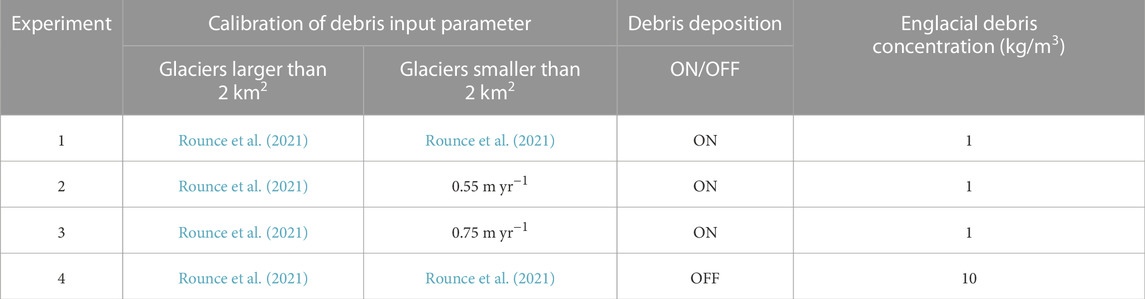
TABLE 2. A set of the conducted sensitivity experiments.

4.1.1 Sensitivity to deposition rate parameters

The sensitivity analysis conducted here explores the effects of different debris deposition rates on the evolution of debris cover and ice volume projections.

If we adopt calibration scheme 1) which utilizes debris thickness data from Rounce et al. (2021) for all glaciers, the deposition rate parameters generally tend to be smaller than 0.55 m yr⁻¹ (refer to Supplementary Figure S5). However, under calibration scheme 2), larger deposition rates are typically applied to glaciers smaller than 2 km². Additionally, we introduced a case where a deposition rate of 0.75 m yr⁻¹ is used in calibration scheme 2 instead of 0.55 m yr⁻¹.

Larger deposition rate parameter has a number of effects on debris cover thickness and area evolution in the XXI century:

• debris cover grows to larger thickness;

• debris cover thickness reaches its maximum later;

• debris cover area is the same until 2022 for the Terek basin and slightly larger for the Kuban basin, albeit by less than 0.7 km²);

• debris cover area after 2022 spans a slightly wider range of values.

At the validation year 2018, the debris cover area for the Terek basin is the same for both calibration schemes. However, for the Kuban basin, calibration scheme 1 underestimates the debris cover area. If a deposition rate of 75 m yr⁻¹ is used instead of 55 m yr⁻¹ in calibration scheme 2, the debris cover area in the Kuban basin will be overestimated, while there is no difference modeled before 2022 for the Terek basin. Consequently, the debris cover area in 2018 in the Kuban basin is more sensitive to the debris cover deposition rate for small glaciers (<2 km²) compared to the Terek basin. Based on the results for the Kuban basin, we assess that calibration scheme 2 with a deposition rate of 55 m yr⁻¹ for glaciers smaller than 2 km² yields the best performance for the debris cover module (refer to Figure 12E).

The ice volume projections, in turn, are also sensitive to debris deposition rate calibration. Compared to results produced under calibration scheme 1, calibration scheme 2 leads to up to 2.5% less ice volume loss in 2020 if deposition rate is set to 0.55 m yr⁻¹ for glaciers smaller than 2 km², and up to 4.5% less ice loss if deposition rate is 0.75 m yr⁻¹ for smaller glaciers. This difference is due to the difference in debris cover thickness since in terms of debris cover area there is no significant difference before 2022. In the future, the lower is the warming, the larger is sensitivity of ice volume projections to deposition rate of debris cover.

Overall, the deposition rate of debris cover has significant effects on debris cover thickness and area evolution in the 21st century. A higher deposition rate leads to thicker debris cover and a delayed peak in thickness. The debris cover area remains relatively stable until 2022, but after that, it spans a slightly wider range of values. Ice volume projections are also sensitive to the calibration of debris deposition rates.

4.1.2 Sensitivity to the meltout component

In our modeling experiments, the distribution of debris cover is primarily influenced by deposition near the top of the glacier and subsequent advection downstream, which modifies the mass balance in the ablation area. The assessment of the meltout component, as outlined in Equation 2, highlights its relatively minor influence on the overall results of the model. This reduced impact can be attributed to the low englacial debris concentration present in the model system. We observe that even if the meltout component was entirely omitted, the resulting effect on the reduction of ablation would be negligible. This finding stems from Equation 2, which facilitates the emergence of debris cover below the equilibrium line altitude (ELA) as soon as debris material is advected to that area. However, it produces realistic debris cover distribution along the glacier.

To assess sensitivity of the results to this model modification, we conducted an additional experiment by disabling the debris cover deposition in Equation 2. In this modified setup, the input of debris cover is solely due to the meltout component. Debris cover is then distributed across a glacier through advection and eventually released to the foreland via the output component. The highest emergence location and rate of the debris cover in this scenario are determined by the mass balance field at each time step. We calibrated the englacial debris cover concentration parameter using a simple trial and error procedure, resulting in a mean value of C_debris = 10 kg/m³. Forward simulations were performed until 2,100.

The results reveal that this model modification, where the debris cover input area coincides with the ablation area and changes over time, fails to accurately reproduce the total debris cover area in 2018. It produces an uneven debris thickness profile, with most of the debris cover concentrated near the glacier terminus, while the debris cover thickness on the remaining glacier area may be underestimated compared to observations from Popovnin et al. (2015). Under this formulation, the fraction of debris-covered ice continues to grow for all scenarios except SSP1-1.9. The warmer the scenario, the greater the fractional growth of debris-covered area by 2,100, reaching 100% under SSP5-8.5 scenario.

Debris thickness becomes four times larger than in the model setup where the deposition component is dominant. However, it should be noted that this outcome contradicts observations of previous debris thickness growth and is likely an artifact of the simplified meltout-driven approach. The predicted regional area-averaged debris cover layer becomes thicker with increasing scenario warmth, although debris cover thickness declines in the second half of the century, similar to the ordinary model setup. For large glaciers, this modification predicts the preservation of ice in 2,100 under debris layers with thickness of several metres, even under the SSP5-8.5 climate scenario (Supplementary Figure S6).

Overall, this ‘meltout-driven’ setup predicts thicker and more extensive debris cover than ‘deposition-driven’ setup. Therefore, the influence of debris cover on ice volume evolution is more pronounced (up to 2%–4%) in this experiment, due to the very large debris thickness accumulation, but it becomes negligible by 2,100 for all scenarios except SSP1-1.9, when considering median values. This suggests that the debris cover’s impact on ice volume is relatively small even if debris is thick and extensive, and that other climate-driven processes play a more dominant role in determining glacier evolution.

In summary, this sensitivity experiment has demonstrated that the ‘deposition-driven’ debris cover module is more robust than its ‘meltout-driven’ counterpart. The meltout component can be safely disregarded, as the model effectively captures this process through the deposition-advection-mass balance correction chain. Future sensitivity tests involving various englacial debris concentration parameters are not deemed necessary based on these findings.

4.2 Debris cover change in the 21st century

The conducted modelling experiments provide insights into the complex dynamics of debris cover thickness in response to varying climate conditions. The changes observed in debris cover thickness throughout the 21st century arise from the interplay between debris accumulation and the release of debris from glaciers into the foreland as a result of glacier retreat, as illustrated in Figures 12A,B.

An interesting finding is the decline in debris cover thickness after 2030–2040 under all climate scenarios until 2,100 (Figures 12A,B). This decline is particularly pronounced under the warmer climate scenarios. The reason may be in a detachment of the thickest parts of the debris cover accumulated at the frontal sections of the glacier during a phase of rapid retreat. Consequently, the deposition of debris cover outside the retreated glacier margins outpaces the rate of debris accumulation on the glacier surface (Figure 15), resulting in a decline in debris cover thickness by 2,100. Under the less aggressive SSP scenarios, a relatively smaller decline in debris cover thickness is sustained after 2040. However, prior to 2030–2040, debris cover thickness experiences growth as debris-covered glaciers undergo slow retreat, influenced by the inverted (and less negative) mass balance gradient in debris-covered frontal areas, which facilitates debris accumulation (Figure 15).

FIGURE 15

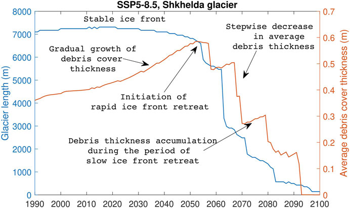
FIGURE 15. Change of glacier length and debris cover thickness of the Shkhelda glacier in the Terek basin under SSP5-8.5 climate scenario. Rapid stepwize decrease of glacier length is associated with detachment of dead ice areas as sufficient ice thinning is achieved.

The conclusion that, on average, debris cover thickness will decrease after 2030–2040 is a novel and debatable finding, considering that to date only increase in debris cover thickness has been observed at the only glacier in the study area where it was measured in the field, (Popovnin et al., 2015). However, we argue that this trend may reverse in the future, since under the warmest scenarios, detachment of large flat areas with previously accumulated debris is predicted. Currently, there is no empirical evidence to validate this projection, as similar occurrences have not been registered in the recent past in the Caucasus. It is important to consider that future trends may differ from past observations, especially under different and warmer climate.

The debris cover thickness predicted under SSP1-1.9 scenario stands out from other simulations. In this case glaciers are able to advance. When glacier advances, the thickest part of debris cover layer next to the glacier front gets distributed along the newly glacierized areas and becomes thinner on average. That leads us to the following negative feedback mechanism:

• Thick debris cover layer accumulated during the preceding retreat and stability phases increases SMB in the frontal area of the glacier;

• As glacier advances, debris cover is stretched along the glacier area and quickly thins (period between 2060 and 2090 in Supplementary Figure S7);

• SMB decreases due to the thinner debris cover, and also due to the lower ice elevation;

• Glacier advance slows down.

Fraction of the debris-covered ice grows while glacier area loss (Supplementary Figure S8) outpaces the loss of debris-bearing areas (Figures 12E,F). However, our modelling results indicate that the expansion of fractional debris cover area will not always be the case in the future compared to the period of glacier retreat in the recent past (Figures 12C,D). In the Terek basin, under all climate scenarios initial growth in the fraction of debris-covered area occurs until 2050, after which it stabilizes for scenarios with lower warming (SSP1-1.9, SSP1-2.6) and continues growing for the warmer ones. This finding suggests that there is a limit to the extent of debris cover expansion in the Caucasus, beyond which the fraction of debris-covered area remains relatively constant. This stabilization can be attributed to the availability of debris material and the equilibrium reached between debris accumulation and removal processes.

Notably, under the warmer SSP3-7.0 and SSP5-8.5 scenarios, the model predicts a significant increase in the debris-covered ice fraction for the Kuban glaciers where it can reach up to 80%. It is important to highlight a strong uncertainty about this result because this trend originates from changes at the Kyukyurtlyu glacier (Mount Elbrus) as almost all other glaciers in the Kuban basin are projected to disappear. If debris cover deposition does not occur at such high elevations after 2050 (5,000 m), it is more likely that debris coverage will decrease rather than expand. This highlights the importance of considering individual glacier dynamics when interpreting the overall trends in debris-covered ice fraction for high-end climate scenarios.

Overall, under the warmer scenarios, the debris cover thickness is projected to decrease, while the proportion of ice covered by debris will expand. This could lead to a larger fraction of thin debris cover potentially resulting in more intensive melt.

4.3 Role of debris cover

We found that the effect of the explicit debris-cover modelling on glacier evolution is not straightforward. The presence of supraglacial debris does not necessarily imply that by 2,100, the simulated ice volume will be larger than ice volume in a debris-free simulation.

In theory, if debris-cover thickness and therefore the melt factor f_debris are the same, larger initial ablation of bare ice will lead to larger impact of the debris cover on ice volume loss. However, the results show the opposite pattern in 2,100: in general, greater differences in ice volume change, simulated using the explicit and implicit debris treatment, are modelled for moderate climate change scenarios (Figure 13). The reason is that glacier may lose connectivity when the dead-ice area is formed (Supplementary Figure S9) or there is more debris release to the foreland than accumulation. As a consequence, the climate scenarios which imply stronger warming lead to a more rapid loss of debris-covered frontal zones of glaciers, which accumulate the thickest debris due to glacier velocity distribution. This results in the same loss of ice volume by 2,100, whether the debris module is included or not, under the warmer scenarios. Under the moderate scenarios, the role of debris cover will be higher than under the extreme scenarios, but the difference between ice volume predicted with and without the debris flow module does not exceed 2 km³ (5% of total ice volume in 2,100). However, the debris cover inhibits melting and retreat of the debris-covered glacier fronts during the century. For example, the projected size of the Bezengi glacier (the largest in the study area) in 2,100 is not much larger when modelled with debris than in the debris-free mode (Supplementary Figure S9). However, in the 2060–2070s (Supplementary Figure S9), the difference in glacier size may be significant. Moreover, when debris is present, large areas of dead ice, detached from the glacier, can survive 10–30 years for the warmest and more moderate scenarios, respectively. This is important for modelling changes in runoff throughout the 21-st century. This result is consistent with the previous studies (Ferguson and Vieli, 2021).

4.4 Dead ice areas

The formation of large areas of dead ice, as predicted by the model, can have important implications for the formation of potentially hazardous lakes. In case of the Bezengi glacier, for example, the model suggests the existence of a substantial dead ice area that may persist for several decades under debris cover, depending on the climate scenario. As lake forms and meltwater continues to accumulate behind the dead ice, water pressure can increase, potentially leading to the destabilization of ice dam and lake outburst.

The timing and volume of water accumulation within the dead ice areas are critical factors in assessing the potential hazard associated with ice-dammed lake formation. The model projections indicate that the largest ice volumes within the dead ice areas are expected to occur between 2030 and 2040, and then a smaller peak is predicted in 2050–2070 depending on climate scenario (Supplementary Figure S4). During this period, the accumulation of meltwater behind the dead ice can reach significant levels, increasing the risk of lake formation and potential outburst floods.

Warmer climate scenarios promote the formation of dead ice (Supplementary Figure S4), as glaciers have less time to adapt compared to colder scenarios. The accelerated recession under warmer conditions can result in the detachment of significant ice areas, leading to formation of dead ice.

It is important to note that the presence of debris cover has an impact on the stability and longevity of the dead ice areas. The insulation provided by debris can delay the melting process, allowing the accumulation of meltwater to persist for a longer duration compared to debris-free scenarios. This extended presence of stagnant ice increases the potential for the development of ice-dammed lakes and subsequent hazards.

4.5 Mass balance change

The mass-balance evolution in the 21st century (Figures 13E,F) is a function of two processes: the future warming (which decreases mass balance) and glacier retreat to higher elevation (which increases mass-balance) Fig. S10). Under the low-emission scenarios, the retreat effect dominates while under the high-emission scenarios, the future warming effect dominates.

It is crucial to distinguish implicit debris-cover implementation (debris-free mode) and the absence of debris cover: an example on Figure 5 shows that if we exclude the implicit influence of debris cover, the difference in ice volume reaches 10% for the Azau Maliy glacier in 20 years. It is, therefore, necessary to account for debris cover in one form or another. A disadvantage of the implicit (debris cover module off) inclusion is that the mass-balance module can take into account the debris-cover geometry at the calibration stage and unable to cope with the fact that debris cover thickness and area evolve in the future.

4.6 Comparison to similar studies

The model presented in this study is the first regional-scale glaciological model, explicitly simulating evolution of supraglacial debris cover using a physically based advection equation which includes the effect of ice dynamics in changing debris extent and thickness. This approach, which incorporates ice dynamics in changing debris extent and thickness, allows for a comprehensive assessment of how variations in temperature and precipitation patterns may affect debris cover thickness and subsequent glacier response at a regional level.

A recent similar study by Compagno et al. (2022) utilizes parameterization for debris thickness evolution and lateral expansion, while neglecting surface velocities when considering the evolution of debris cover. This means that the mass balance modification due to debris cover is calculated independently of ice flow dynamics. In contrast, our study directly links the debris cover module with ice dynamics, requiring simultaneous model runs. It has been shown that debris cover advection plays a significant role in the thickening of debris in response to climate change (Anderson et al., 2021). Particularly, the patterns of debris thickness are strongly controlled by the decrease in surface velocity downglacier (Kirkbride, 2000; Anderson and Anderson, 2018; Ferguson and Vieli, 2021). Therefore, the dynamic effects on debris thickness are especially important in areas where surface velocities are low and debris cover tends to be thick. This implies that debris cover may thicken substantially in locations where the parameterizations presented in Compagno et al. (2022) do not account for it.

This study has shown that the debris cover has limited influence on the ice-volume evolution in the 21-st century, which is in line with the recent research (Fleischer et al., 2021; Compagno et al., 2022; Rounce et al., 2023). In Rounce et al. (2023), where the debris cover was taken into account in a constant state, described in Rounce et al. (2021), the effect of debris cover was quantified as less than 5%, which is consistent with our study.

However, the use of debris-cover module may be particularly important for the tasks where glacier front position is required, e.g., glacial lakes. Our study predicts that during the 21st century, the length of individual large glaciers can be significantly larger if debris cover is modelled explicitly. This result is consistent with earlier modelling studies (Ferguson and Vieli, 2021; Compagno et al., 2022) and observations (Pellicciotti et al., 2015) which illustrate that the response of the debris-covered glaciers is pronounced in glacier length rather than ice volume (Fig. S11).

Debris cover influences changes in glacier geometry change, mass-balance gradient, ice velocity and hence the driving-stress field. The debris-cover influence on the these characteristics relative to initial debris-free glaciers is consistent with Anderson and Anderson (2016) and Ferguson and Vieli (2021):

• the debris thickness increases down glacier from the deposition location and creates the reversed mass balance gradient (Figure 6B);

• ice velocity gradient of the debris-covered glaciers is reduced relative to debris-free glaciers in the ablation zone (Figure 8);

• ice surface velocity at debris-covered termini is concave upward while for debris-free glacier it is convex up near the glacier terminus (Figure 8)

• debris-covered glaciers tend to lose volume first by downwasting followed by retreat.

Although Anderson and Anderson (2016) and Ferguson and Vieli (2021) has shown that the debris cover has a large effect on changes in glacier size, in our projections glaciers tend to have similar volumes by 2,100. That result points to the difference between simulations using climate projections and steady climate. When projections are utilized, the difference in glacier geometries with or without debris cover is smaller due to rapid glacier retreat to higher elevations.

The median projected area change after 2030 coincides with values presented in Rounce et al. (2023) for the Terek and Kuban basins (Supplementary Figure S14). However, for the Kuban basin the gradient of predicted area decline is larger in Rounce et al. (2021) in the first half of the century. It is important to note that the pattern of area change may vary significantly for individual glaciers. As a general trend, Rounce et al. (2023) suggests a steeper area decline compared to our study, possibly because they consider fixed debris cover geometry from 2008, which quickly disappears if fixed in space.

5 Conclusion

In this study, we presented a new debris cover module which was coupled to the GloGEMflow model and can be used on a regional scale. The debris thickness evolves by means of meltout from the glacier and dynamic re-distribution. Debris cover deposition rate was calibrated using debris thickness dataset (Rounce et al., 2021). The fractional debris-covered area changes with time under the influence of the growth factor which also evolves depending on the frontal debris thickness. This growth-factor dependency was calibrated using the newly-mapped debris cover outlines. The mass balance was calibrated for either implicit or explicit debris-cover formulation, and the results of application of both methods were compared.

The model was applied to glaciers in the Northern Caucasus belonging to the catchments of Terek and Kuban rivers. Terek and Kuban basins differ in terms of ice volume loss rate. In the Kuban basin, glaciers lose ice almost two times quicker than in the Terek basin in the first half of the century. One-third of ice observed in 2015 will be lost in the Terek basin by 2035, while in the Kuban basin, it is predicted to happen already in 2025. In the Terek basin, between 43% ± 27% (SSP5-8.5) and 98% ± 1% (SSP1-1.9) of 2015 ice volume will be left in 2,100. In the Kuban basin, between 63% ± 36% (SSP5-8.5) and 99% ± 2% (SSP1-1.9) of ice volume will be left by 2,100. The ice volume stabilizes under SSP1-1.9 scenario in 2040, which is an important result, given there is still time for the world to meet their obligations under the Paris Climate Agreement and keep warming to 1.5 C. Under the extreme climate scenarios, glacier ice disappears almost everywhere except Mount Elbrus by 2,100. Under the moderate climate scenarios, ice volume stabilizes at lower elevations. Despite the differences due to modelling with or without debris cover module being small (up to 4.5% in the Terek basin and up to 2.5% in the Kuban basin), in general, the projected loss tends to be less pronounced when debris cover is modelled explicitly.

The study demonstrates similar patterns of debris cover change over time in the Terek and Kuban regions. As expected, warmer climates result in more debris covered ice. However, the model predicts thinner debris cover for warmer climates due to rapid terminus retreat after 2030–2040 and subsequent wastage of thick debris cover at the glacier fronts.

To assess the debris-cover effect on glacier evolution, it is not enough to trace the final results of the simulation for 2,100. As a rule, the maximum difference in glacier parameters depending on the debris-loaded or debris-free modelling mode occurs before 2,100, especially for large valley glaciers but by the end of the century it is eliminated due to the retreat of debris-bearing parts of the glaciers or due to the elevation-stabilization effect (if the glacier with implicitly-modelled debris retreats higher in the first half of the century, it will experience less-negative mass balance in the second part of the century). Even if other debris cover model modifications are used, which allow for fractional debris covered area growth until 2,100, the effect of debris cover on ice volume will still be negligible compared to climate scenario uncertainty by the end of the century.

The explicit debris-cover simulation serves to improve our understanding of the future glacier evolution. In an attempt to evaluate how “wrong” glacier models without explicit debris-cover formulation are, we conclude the following.

• if the large-scale ice volume change needs to be assessed, the implicit treatment of debris cover produces acceptable results, however debris cover contributes up to 5% to the estimation of error and uncertainty in models of debris-covered glacier change;

• if the geometry and the dynamics of the glaciers (terminus location, mass balance, surface velocity, driving stress) is important, explicit debris-cover treatment is preferrable (one of important examples is ice-thickness estimation based on mass continuity).

The sensitivity experiments demonstrated that the deposition-driven debris cover module is more reliable and accurate than its meltout-driven counterpart. This finding suggests that the deposition process, where debris cover is deposited onto the glacier surface and subsequently advected downstream, plays a dominant role in determining the distribution and thickness of debris cover.

Debris-cover wastage further facilitates the formation of moraine-dammed lakes with possible dead-ice inclusion, which in turn creates favourable conditions for outburst floods due to the dam instability (Petrakov et al., 2008; Benn et al., 2012). A newly introduces debris-cover module for GloGEMflow model provides an opportunity to predict areas of dead ice and proglacial lakes formation in the future, as glaciers recede. Between 2030 and 2040, the model projections indicate a peak in ice volumes within the dead ice areas, on a regional level. This period may correspond to significant meltwater accumulation behind the stagnant ice, heightening the potential for lake formation and the associated risk of outburst floods. Such information is essential for implementing effective early warning systems and developing appropriate mitigation measures to minimize the potential impacts on downstream communities and infrastructure.

Data availability statement

The raw data supporting the conclusion of this article will be made available by the authors, without undue reservation.

Author contributions

TP: Conceptualization, Formal Analysis, Investigation, Methodology, Software, Validation, Visualization, Writing–original draft. OR: Conceptualization, Supervision, Writing–review and editing, Funding acquisition, Project administration. AG: Data curation, Writing–review and editing. HZ: Software, Writing–review and editing. MH: Data curation, Software, Writing–review and editing, Conceptualization. MS: Writing–review and editing, Conceptualization, Funding acquisition, Project administration.

Funding

The author(s) declare financial support was received for the research, authorship, and/or publication of this article. The reported study was funded by RFS, project number 22-17-00133. TP got support from RFBR according to the research project no. 20-35-90042.

Acknowledgments

This study was carried out under Governmental Order to Water Problems Institute, Russian Academy of Sciences, subject no. FMWZ- 2022–0001.

Conflict of interest

The authors declare that the research was conducted in the absence of any commercial or financial relationships that could be construed as a potential conflict of interest.

Publisher’s note

All claims expressed in this article are solely those of the authors and do not necessarily represent those of their affiliated organizations, or those of the publisher, the editors and the reviewers. Any product that may be evaluated in this article, or claim that may be made by its manufacturer, is not guaranteed or endorsed by the publisher.

Supplementary material

The Supplementary Material for this article can be found online at: https://www.frontiersin.org/articles/10.3389/feart.2023.1256696/full#supplementary-material

References

Anderson, L. S., and Anderson, R. S. (2018). Debris thickness patterns on debris-covered glaciers. Geomorphology 311, 1–12. doi:10.1016/j.geomorph.2018.03.014

CrossRef Full Text | Google Scholar

Anderson, L. S., and Anderson, R. S. (2016). Modeling debris-covered glaciers: response to steady debris deposition. Cryosphere 10, 1105–1124. doi:10.5194/tc-10-1105-2016

CrossRef Full Text | Google Scholar

Anderson, L. S., Armstrong, W. H., Anderson, R. S., and Buri, P. (2021). Debris cover and the thinning of kennicott glacier, Alaska: in situ measurements, automated ice cliff delineation and distributed melt estimates. Cryosphere 15, 265–282. doi:10.5194/tc-15-265-2021

CrossRef Full Text | Google Scholar

Banerjee, A., and Shankar, R. (2013). On the response of himalayan glaciers to climate change. J. Glaciol. 59, 480–490. doi:10.3189/2013jog12j130

CrossRef Full Text | Google Scholar

Benn, D., Bolch, T., Hands, K., Gulley, J., Luckman, A., Nicholson, L., et al. (2012). Response of debris-covered glaciers in the mount everest region to recent warming, and implications for outburst flood hazards. Earth-Science Rev. 114, 156–174. doi:10.1016/j.earscirev.2012.03.008

CrossRef Full Text | Google Scholar

Benn, D. I., and Lehmkuhl, F. (2000). Mass balance and equilibrium-line altitudes of glaciers in high-mountain environments. Quat. Int. 65-66, 15–29. doi:10.1016/S1040-6182(99)00034-8

CrossRef Full Text | Google Scholar

Bozhinskiy, A., Krass, M., and Popovnin, V. (1986). Role of debris cover in the thermal physics of glaciers. J. Glaciol. 32, 255–266. doi:10.3189/S0022143000015598

CrossRef Full Text | Google Scholar

Brun, F., Wagnon, P., Berthier, E., Jomelli, V., Maharjan, S., Shrestha, F., et al. (2019). Heterogeneous influence of glacier morphology on the mass balance variability in high mountain asia. J. Geophys. Res. Earth Surf. 124, 1331–1345. doi:10.1029/2018jf004838

CrossRef Full Text | Google Scholar

Brun, F., Wagnon, P., Berthier, E., Shea, J. M., Immerzeel, W. W., Kraaijenbrink, D., et al. (2018). Can ice-cliffs explain the “debris-cover anomaly”? new insights from changri nup glacier, Nepal, central himalaya. Cryosphere Discuss., 1–32. doi:10.5194/tc-2018-38

CrossRef Full Text | Google Scholar

Compagno, L., Huss, M., Miles, E. S., McCarthy, M. J., Zekollari, H., Pellicciotti, F., et al. (2022). Modelling supraglacial debris-cover evolution from the single glacier to the regional scale: an application to high mountain asia. Cryosphere Discuss. 1, 1697–1718. doi:10.5194/tc-16-1697-2022

CrossRef Full Text | Google Scholar

Eyring, V., Bony, S., Meehl, G. A., Senior, C. A., Stevens, B., Stouffer, R. J., et al. (2016). Overview of the coupled model intercomparison project phase 6 (cmip6) experimental design and organization. Geosci. Model Dev. 9, 1937–1958. doi:10.5194/gmd-9-1937-2016

CrossRef Full Text | Google Scholar

Ferguson, J. C., and Vieli, A. (2021). Modelling steady states and the transient response of debris-covered glaciers. Cryosphere 15, 3377–3399. doi:10.5194/tc-15-3377-2021

CrossRef Full Text | Google Scholar

Fleischer, F., Otto, J.-C., Junker, R., and Hölbling, D. (2021). Evolution of debris cover on glaciers of the eastern alps, Austria, between 1996 and 2015. Earth Surf. Process. Landforms 46, 1673–1691. doi:10.1002/esp.5065

CrossRef Full Text | Google Scholar

Fujita, K., and Sakai, A. (2014). Modelling runoff from a himalayan debris-covered glacier. Hydrology Earth Syst. Sci. 18, 2679–2694. doi:10.5194/hess-18-2679-2014

CrossRef Full Text | Google Scholar

Haeberli, W., Frauenfelder, R., Hoelzle, M., and Zemp, M. (2003). Glacier mass balance bulletin no. 7, 2000–2001. IAHS (ICSI), Zürich.

Google Scholar

Hambrey, M. J., Quincey, D. J., Glasser, N. F., Reynolds, J. M., Richardson, S. J., and Clemmens, S. (2008). Sedimentological, geomorphological and dynamic context of debris-mantled glaciers, mount everest (sagarmatha) region, Nepal. Quat. Sci. Rev. 27, 2361–2389. doi:10.1016/j.quascirev.2008.08.010

CrossRef Full Text | Google Scholar

Herreid, S., and Pellicciotti, F. (2020). The state of rock debris covering earth’s glaciers. Nat. Geosci. 13, 621–627. doi:10.1038/s41561-020-0615-0

CrossRef Full Text | Google Scholar

Hersbach, H., Bell, B., Berrisford, P., Horányi, A., Sabater, J. M., Nicolas, J., et al. (2019). Global reanalysis: goodbye era-interim, hello era5. ECMWF Newsl. 159, 17–24. doi:10.21957/vf291hehd7

CrossRef Full Text | Google Scholar

Huang, L., Li, Z., Han, H., Tian, B., and Zhou, J. (2018). Analysis of thickness changes and the associated driving factors on a debris-covered glacier in the tienshan mountain. Remote Sens. Environ. 206, 63–71. doi:10.1016/j.rse.2017.12.028

CrossRef Full Text | Google Scholar

Hugonnet, R., McNabb, R., Berthier, E., Menounos, B., Nuth, C., Girod, L., et al. (2021). Accelerated global glacier mass loss in the early twenty-first century. Nature 592, 726–731. doi:10.1038/s41586-021-03436-z

PubMed Abstract | CrossRef Full Text | Google Scholar

Huss, M., and Farinotti, D. (2012). Distributed ice thickness and volume of all glaciers around the globe: GLOBAL GLACIER ICE THICKNESS AND VOLUME. J. Geophys. Res. Earth Surf. 117. doi:10.1029/2012JF002523

CrossRef Full Text | Google Scholar

Huss, M., and Hock, R. (2015). A new model for global glacier change and sea-level rise. Front. Earth Sci. 3, 54. doi:10.3389/feart.2015.00054

CrossRef Full Text | Google Scholar

Hutter, K. (1983). “The application of the shallow-ice approximation,” in Theoretical glaciology (Springer), 256–332.

CrossRef Full Text | Google Scholar

Immerzeel, W., Pellicciotti, F., and Bierkens, M. (2013). Rising river flows throughout the twenty-first century in two himalayan glacierized watersheds. Nat. Geosci. 6, 742–745. doi:10.1038/ngeo1896

CrossRef Full Text | Google Scholar

IPCC (2021). Climate change 2021: the physical science basis. contribution of working group14 i to the sixth assessment report of the intergovernmental panel on climate change; technical summary.

Google Scholar

IPCC (2022). High Mountain areas. Cambridge University Press, 144. doi:10.1017/9781009157964.004

CrossRef Full Text | Google Scholar

Khromova, T., Nosenko, G., Glazovsky, A., Nikitin, S., and Muraviev, A. (2020). “New glacier inventory of the Russian glaciers based on sentinel images (2017/2018),” in EGU General Assembly Conference Abstracts.21056

Google Scholar

Kirkbride, M. P. (2000). Ice-marginal geomorphology and holocene expansion of debris-covered tasman glacier. N. Z. IAHSAISH P 264, 211–217.

Google Scholar

Konrad, S. K., and Humphrey, N. F. (2000). Steady-state flow model of debris-covered glaciers (rock glaciers). Iahs Publication, 255–266.

Google Scholar

Kraaijenbrink, P. D., Bierkens, M., Lutz, A., and Immerzeel, W. (2017). Impact of a global temperature rise of 1.5 degrees celsius on asia’s glaciers. Nature 549, 257–260. doi:10.1038/nature23878

PubMed Abstract | CrossRef Full Text | Google Scholar

Kutuzov, S., Lavrentiev, I., Smirnov, A., Nosenko, G., and Petrakov, D. (2019). Volume changes of elbrus glaciers from 1997 to 2017. Front. Earth Sci. 153. doi:10.3389/feart.2019.00153

CrossRef Full Text | Google Scholar

Kutuzov, S., Shahgedanova, M., Krupskaya, V., and Goryachkin, S. (2021). Optical, geochemical and mineralogical characteristics of light-absorbing impurities deposited on djankuat glacier in the caucasus mountains. Water 13, 2993. doi:10.3390/w13212993

CrossRef Full Text | Google Scholar

Mayer, C., and Licciulli, C. (2021). The concept of steady state, cyclicity and debris unloading of debris-covered glaciers. Front. Earth Sci. 9, 896. doi:10.3389/feart.2021.710276

CrossRef Full Text | Google Scholar

Mertes, J. R., Thompson, S. S., Booth, A. D., Gulley, J. D., and Benn, D. I. (2017). A conceptual model of supra-glacial lake formation on debris-covered glaciers based on gpr facies analysis. Earth Surf. Process. Landforms 42, 903–914. doi:10.1002/esp.4068

CrossRef Full Text | Google Scholar

Millan, R., Mouginot, J., Rabatel, A., and Morlighem, M. (2022). Ice velocity and thickness of the world’s glaciers. Nat. Geosci. 15, 124–129. doi:10.1038/s41561-021-00885-z

CrossRef Full Text | Google Scholar

Mölg, N., Bolch, T., Rastner, P., Strozzi, T., and Paul, F. (2018). A consistent glacier inventory for karakoram and pamir derived from landsat data: distribution of debris cover and mapping challenges. Earth Syst. Sci. Data 10, 1807–1827. doi:10.5194/essd-10-1807-2018

CrossRef Full Text | Google Scholar

Nuimura, T., Fujita, K., Yamaguchi, S., and Sharma, R. R. (2012). Elevation changes of glaciers revealed by multitemporal digital elevation models calibrated by gps survey in the khumbu region, Nepal himalaya, 1992-2008. J. Glaciol. 58, 648–656. doi:10.3189/2012jog11j061

CrossRef Full Text | Google Scholar

O’Neill, B. C., Tebaldi, C., Van Vuuren, D. P., Eyring, V., Friedlingstein, P., Hurtt, G., et al. (2016). The scenario model intercomparison project (scenariomip) for cmip6. Geosci. Model Dev. 9, 3461–3482. doi:10.5194/gmd-9-3461-2016

CrossRef Full Text | Google Scholar

Østrem, G. (1959). Ice melting under a thin layer of moraine, and the existence of ice cores in moraine ridges. Geogr. Ann. 41, 228–230. doi:10.1080/20014422.1959.11907953

CrossRef Full Text | Google Scholar

Paul, F., and Haeberli, W. (2008). Spatial variability of glacier elevation changes in the swiss alps obtained from two digital elevation models. Geophys. Res. Lett. 35, L21502. doi:10.1029/2008gl034718

CrossRef Full Text | Google Scholar

Pellicciotti, F., Stephan, C., Miles, E., Herreid, S., Immerzeel, W. W., and Bolch, T. (2015). Mass-balance changes of the debris-covered glaciers in the langtang himal, Nepal, from 1974 to 1999. J. Glaciol. 61, 373–386. doi:10.3189/2015jog13j237

CrossRef Full Text | Google Scholar

Petrakov, D., Chernomorets, S., Evans, S., and Tutubalina, O. (2008). Catastrophic glacial multi-phase mass movements: a special type of glacial hazard. Adv. Geosciences 14, 211–218. doi:10.5194/adgeo-14-211-2008

CrossRef Full Text | Google Scholar

Popovnin, V., Rezepkin, A., and Tielidze, L. (2015). Superficial moraine expansion on the djankuat glacier snout over the direct glaciological monitoring period. Earth Cryosphere 19, 79–87.

Google Scholar

Reznichenko, N., Davies, T., Shulmeister, J., and McSaveney, M. (2010). Effects of debris on ice-surface melting rates: an experimental study. J. Glaciol. 56, 384–394. doi:10.3189/002214310792447725

CrossRef Full Text | Google Scholar

RGI Consortium (2017). Echnical report, global land ice measurements from space. Colorado, USA: Digital Media. July: 1–14.Randolph glacier inventory–a dataset of global glacier outlines: version 6.0.

Google Scholar

Rounce, D. R., Hock, R., Maussion, F., Hugonnet, R., Kochtitzky, W., Huss, M., et al. (2023). Global glacier change in the 21st century: every increase in temperature matters. Science 379, 78–83. doi:10.1126/science.abo1324

PubMed Abstract | CrossRef Full Text | Google Scholar

Rounce, D. R., Hock, R., McNabb, R., Millan, R., Sommer, C., Braun, M., et al. (2021). Distributed global debris thickness estimates reveal debris significantly impacts glacier mass balance. Geophys. Res. Lett. 48, e2020GL091311. doi:10.1029/2020GL091311

PubMed Abstract | CrossRef Full Text | Google Scholar

Rowan, A. V., Egholm, D. L., Quincey, D. J., and Glasser, N. F. (2015). Modelling the feedbacks between mass balance, ice flow and debris transport to predict the response to climate change of debris-covered glaciers in the himalaya. Earth Planet. Sci. Lett. 430, 427–438. doi:10.1016/j.epsl.2015.09.004

CrossRef Full Text | Google Scholar

Sakai, A., Takeuchi, N., Fujita, K., and Nakawo, M. (2000). Role of supraglacial ponds in the ablation process of a debris-covered glacier in the Nepal himalayas. IAHS PUBLICATION, 119–132.

Google Scholar

Scherler, D., Wulf, H., and Gorelick, N. (2018). Global assessment of supraglacial debris-cover extents. Geophys. Res. Lett. 45, 11–798. doi:10.1029/2018GL080158

CrossRef Full Text | Google Scholar

Shahgedanova, M., Nosenko, G., Kutuzov, S., Rototaeva, O., and Khromova, T. (2014). Deglaciation of the caucasus mountains, Russia/georgia, in the 21st century observed with aster satellite imagery and aerial photography. Cryosphere 8, 2367–2379. doi:10.5194/tc-8-2367-2014

CrossRef Full Text | Google Scholar

Srocc, I. (2019). The ocean and cryosphere in a changing climate, 625. WMO and UNEP. chapter 2: High mountain areas.

Google Scholar

Stokes, C. R., Gurney, S. D., Shahgedanova, M., and Popovnin, V. (2006). Late-20th-century changes in glacier extent in the caucasus mountains, Russia/georgia. J. Glaciol. 52, 99–109. doi:10.3189/172756506781828827

CrossRef Full Text | Google Scholar

Tielidze, L. G., Bolch, T., Wheate, R. D., Kutuzov, S. S., Lavrentiev, I. I., and Zemp, M. (2020). Supra-glacial debris cover changes in the greater caucasus from 1986 to 2014. Cryosphere 14, 585–598. doi:10.5194/tc-14-585-2020

CrossRef Full Text | Google Scholar

Tielidze, L. G., Nosenko, G. A., Khromova, T. E., and Paul, F. (2022). Strong acceleration of glacier area loss in the greater caucasus between 2000 and 2020. Cryosphere 16, 489–504. doi:10.5194/tc-16-489-2022

CrossRef Full Text | Google Scholar

Tielidze, L. G., and Wheate, R. D. (2018). The greater caucasus glacier inventory (Russia, Georgia and Azerbaijan). Cryosphere 12, 81–94. doi:10.5194/tc-12-81-2018

CrossRef Full Text | Google Scholar

Trüssel, B. L., Truffer, M., Hock, R., Motyka, R. J., Huss, M., and Zhang, J. (2015). Runaway thinning of the low-elevation yakutat glacier, Alaska, and its sensitivity to climate change. J. Glaciol. 61, 65–75. doi:10.3189/2015jog14j125

CrossRef Full Text | Google Scholar

Vaughan, D., Stocker, T., Qin, D., Plattner, G., Tignor, M., Allen, S., et al. (2013). Climate change: the physical science basis. contribution of working group i to the fifth assessment report of the intergovernmental panel on climate change.

Google Scholar

Verhaegen, Y., Huybrechts, P., Rybak, O., and Popovnin, V. V. (2020). Modelling the evolution of djankuat glacier, north caucasus, from 1752 until 2100 ce. Cryosphere 14, 4039–4061. doi:10.5194/tc-14-4039-2020

CrossRef Full Text | Google Scholar

Volodicheva, N. (2002). The caucasus. Phys. Geogr. North. Eurasia, 350–376.

Google Scholar

Winter-Billington, A., Moore, R., and Dadic, R. (2020). Evaluating the transferability of empirical models of debris-covered glacier melt. J. Glaciol. 66, 978–995. doi:10.1017/jog.2020.57

CrossRef Full Text | Google Scholar

Zekollari, H., Huss, M., and Farinotti, D. (2019). Modelling the future evolution of glaciers in the european alps under the euro-cordex rcm ensemble. Cryosphere 13, 1125–1146. doi:10.5194/tc-13-1125-2019

CrossRef Full Text | Google Scholar

Zekollari, H., Huss, M., and Farinotti, D. (2020). On the imbalance and response time of glaciers in the european alps. Geophys. Res. Lett. 47, e2019GL085578. doi:10.1029/2019gl085578

CrossRef Full Text | Google Scholar

Zekollari, H., Huybrechts, P., Fürst, J., Rybak, O., and Eisen, O. (2013). Calibration of a higher-order 3-d ice-flow model of the morteratsch glacier complex, engadin, Switzerland. Ann. Glaciol. 54, 343–351. doi:10.3189/2013aog63a434

CrossRef Full Text | Google Scholar

Zemp, M., Nussbaumer, S. U., Gärtner-Roer, I., Bannwart, J., Paul, F., and Hoelzle, M. (2021). Global glacier change bulletin nr. 4 (2018–2019). WGMS 4.

Google Scholar

Zhang, Y., Gu, J., Liu, S., Wang, X., Jiang, Z., Wei, J., et al. (2022). Spatial pattern of the debris-cover effect and its role in the hindu kush-pamir-karakoram-himalaya glaciers. J. Hydrology 615, 128613. doi:10.1016/j.jhydrol.2022.128613

CrossRef Full Text | Google Scholar