Unraveling the coupled HighResMIP-CMIP6 models resolution impacts in present climate and future projections of water availability over South America

This study examines present and future projections of precipitation and evapotranspiration for South America, focusing on small regions with distinct environmental and climatic characteristics. The objective is to understand future water availability across the continent and assess the role of model resolution in shaping these projections (2015–2050). Five coupled Global Coupled Climate Models (GCMs) from CMIP6 (HighResMIP) with low (∼70 km) and high (∼25 km) horizontal resolutions were analyzed: HadGEM3, MPI, CMCC, EC-Earth3P, and HiRAM. For the present climate (1979–2014), statistical indices were applied to identify the primary effects of model resolution on the ability to capture regional climate characteristics by comparing simulations with GPCC and ERA5 reference dataset. The HighResMIP models demonstrated strong performance in simulating the precipitation climatology, with higher-resolution versions increasing the spatial pattern correlation (until 0.90) and reducing the RMSE (1.32 to 1.82 mm/day) and biases. These spatial correlations improved further (until 0.93) when only precipitation over continental areas is analyzed. At the regional scale, the precipitation annual cycles in high-resolution simulations is consistently improved over the northeast Brazil, La Plata basin and eastern Amazon basin, while in others regions the differences between high and low resolutions are smaller as well as occurs for evapotranspiration annual cycles except in eastern Amazon. In both resolutions, projections indicate a future intensification of the dry season, with a rainfall decrease of over 30% in central South America. For austral summer and autumn, a future increase of rainfall is projected for Pacific and Atlantic branches and southward of 25°S, including La Plata basin. The future changes in water resources present some differences associated with model resolution. The high-resolution projects water resources increased in an extensive strip from central Argentina to northeastern Brazil and decreased over the Amazon basin. For low-resolution projections this change pattern is not so evident due large divergence between members. The signal of precipitation and evapotranspiration trends controlling the water resources trends at a regional scale, previously found only in regional climate projections, is consistent with those in high-resolution HighResMIP simulations.

1 Introduction

Recent extreme weather events worldwide have alerted society to the impacts of climate change (Clarke et al., 2022; Kornhuber et al., 2018). The severe social consequences of the extreme rainfall events in urban and rural areas, along with prolonged drought, are straining water availability for populations, ecosystems and food production. In South America, these effects manifest in varied ways, depending on the region (Hoyos et al., 2013). These impacts underscore larger global challenges, highlighting the need for advanced climate models to better capture the complex interactions between land use and hydrological changes.

At climate scale, water resources (WR), or water availability, in any region are fundamentally determined by the balance between precipitation (P) and evapotranspiration (ET), as these are the primary components of the hydrological cycle (Llopart et al., 2019). WR are critical for sustaining both human life and ecosystems, especially in a rapidly changing world where demand, pollution, and climate impacts are intensifying. A great example is the Pantanal, one of the largest continuous wetland areas in the world (Junk and Cunha, 2005), located in central South America. This region faces severe devastation due to the increased wildfire frequency (Libonati et al., 2021), a crisis that is further aggravated by land-use changes, particularly the expansion of agriculture, which is replacing natural vegetation and diminishing wetland areas. According to the latest MapBiomas (2024) survey, the Pantanal has seen a reduction in its water-covered area and a lengthening of dry periods. This shift not only reduces the flooded area but also heightens the region’s vulnerability to wildfires. Connected to the Pantanal is the La Plata Basin (LPB), which has been significantly impacted by large variability in water regimes and extreme rainfall events (Carril et al., 2016). LPB is an important region on the continent, both demographically and economically, spanning southeast-south Brazil, Paraguay, Uruguay and northern Argentina. South America is also home to the Amazon Basin, the world’s largest hydrological basin within a tropical forest, essential to the hydrological systems across the continent (Marengo, 2006; Rehbein and Ambrizzi, 2023).

The great north-south extension of South America, its relief, and different ecosystems contribute significantly to the characterization of its different climate regimes (Reboita et al., 2010), presenting additional challenges to climate simulations. While Global Climate Models (GCMs) projections are crucial for studying future climate changes, they have inherent limitations in simulating the dynamics and other physical processes. This introduces uncertainties in the climate representation (Sampaio and Dias, 2014), particularly in regions with complex topographies where simulation biases tend to increase (Avila-Diaz et al., 2020; Ito et al., 2020). To address these uncertainties, the Coupled Model Intercomparison Project (CMIP - Meehl, 1995), launched in 1995 and organized under the Working Group on Coupled Modelling (WGCM) of the World Climate Research Programme (WCRP), provides a platform where the scientific community can analyse simulations from different GCMs to assess their ability to represent the present climate and future climate change scenarios. The project organizes climate projections using both atmospheric-only and coupled ocean-atmosphere GCMs and their responses to different idealized greenhouse gas forcings. The current phase of CMIP6 (Eyring et al., 2016) was built upon advancements from previous iterations and incorporates the use of Shared Socioeconomic Pathways (SSPs). SSPs are integrated scenarios that outline different potential trajectories for global socioeconomic development, including factors such as population growth, economic development, energy use, and land use, to explore future climate change and its impacts (O’Neill et al., 2017).

CMIP-GCMs still run with relatively coarse horizontal resolution, which increased from an average of ∼250–300 km in CMIP3 to ∼100–150 km in CMIP6 (Haarsma et al., 2016). However, these resolutions are still relatively coarse, potentially contributing to uncertainties in the climate projections over South America (Ortega et al., 2021; Firpo et al., 2022; Bazzanela et al., 2023). In order to reduce uncertainty associated with the low GCM resolutions, CMIP6 introduced a special set of simulations called HighResMIP (High-Resolution Model Intercomparison Project), where GCMs would be executed with a spatial resolution of ∼25 to 50 km in the atmosphere, focusing on the impacts of resolution on the origin and consequences of systematic model biases (Haarsma et al., 2016).

Studies have assessed HighResMIP performance worldwide and for some different regions of the world. A first evaluation of the coupled HighResMIP simulations over the entire globe did not find substantial differences in the annual mean biases of rainfall, temperature or cloud cover as a function of model resolution (Moreno-Chamarro et al., 2021). Bock et al. (2020) provided valuable insights into the evaluation of precipitation projections across different climate model ensembles by assessing a large number of models from CMIP3, CMIP5, CMIP6, and HighResMIP. Bock et al. (2020) highlighted improvements in precipitation with important bias reduction in the Pacific and equatorial Atlantic regions for HighResMIP. Additionally, they demonstrate a progressive increase in global precipitation correlation with observations from CMIP3 to CMIP6, underlining the advancements in modeling capabilities. Ajibola et al. (2020), Li et al. (2021) both evaluated atmospheric-only GCMs from the HighResMIP project, with Ajibola et al. (2020) focusing on daily precipitation climatology in West Africa and Li et al. (2021) assessing precipitation projections for Central Asia, finding generally high correlations with observed data, though with some models showing lower performance in both regions. Avila-Diaz et al. (2023) and Negrón-Juárez et al. (2024) evaluated atmospheric-only HighResMIP projections for South America and the Caribbean using climate extreme indices. Avila-Diaz et al. (2023) compared models performance in representing current climate for temperature and precipitation indices, with no significant differences found between higher and lower resolution simulations when compared to ERA5 and CHIRPS data. Focusing only in the Amazon region, Negrón-Juáez et al. (2024) discussed that most HighResMIP models are able to reproduce the observed extreme daily precipitation events, but not these events in the sub-daily time scales.

In the context of model resolution effect in the near surface variables, some studies have compared GCMs and regional climate models (RCMs) simulations. The future WR projections to the end of the 21st century provided by GCM and RCM ensembles over South America were investigated by Llopart et al. (2019). An important outcome is the larger area with increasing water availability projected by the RCMs compared to the GCM ensemble. This discrepancy resulted in future changes with signal disagreement between RCMs and GCMs over central-western Brazil, including Pantanal and Cerrado regions. While the GCMs ensemble projected a WR decrease, the RCM ensemble indicated an increase by the end of the 21st century. This divergence was attributed to the higher resolution of the RCMs (Llopart et al., 2019). In a later work, using CMIP5-GCMs and higher resolution RCMs from CORDEX-CORE experiment (Coordinated Output for Regional Evaluations from Coordinated Regional Climate Downscaling; Giorgi et al. (2021), Llopart et al. (2020) found for the end of the 21-century a more intense decreasing (increasing) in water availability in Amazon basin (La Plata basin) in RCMs than GCMs during austral summer. This highlights again the role of model resolution on future changes of moisture availability.

Up to date, no evaluation of coupled GCMs from HighResMIP was conducted to understand the impact of model resolution in South America climate. This work aims to further advance on understanding coupled HighResMIP resolution impacts on representation of near surface variables (precipitation, evapotranspiration and water availability) in the present climate and mid-21st century projections over South America. Special attention is given to the role of model resolution on climatology and projections of water balance on key-regions of the continent, selected considering their environmental, social and economic aspects. To this end, for the first time five coupled GCM from HighResMIP-CMIP6 with high and low-resolutions and observational datasets are used in this study.

2 Materials and methods

2.1 Observational data

The European Center for Medium-Range Weather Forecasts (ECMWF) ERA5 reanalysis (Hersbach et al., 2020) has been used to evaluate CMIP6 projections due to its temporal and spatial coverage, as well as its available resolution. This study uses monthly precipitation and evapotranspiration data from ERA5 over the South America continent and adjacent oceans with a horizontal resolution of 0.25°. For continental areas, the gauge based precipitation data from the Global Precipitation Climatology Centre (GPCC; Schneider et al., 2015) with 0.25° horizontal resolution is also used. To verify the consistency of the climatology provided by ERA5 and GPCC, these datasets are compared with Integrated Multi-satellitE Retrievals (IMERG) data, latest version (V07) of Global Precipitation Measurement Mission (GPM) IMERG Final Run product produced by National Aeronautics and Space Administration (NASA) Goddard Space Flight Center (GSFC; Huffman et al., 2019), which provides precipitation at 0.1° × 0.1° spatial resolution in the period 2000–2014. IMERG is considered the state-of-the-art rainfall estimation (Asong et al., 2017; Pradhan et al., 2022) with fine-resolution covering the entire globe. For instance, Tao et al. (2022) used IMERG to evaluate the diurnal cycle of monsoons simulated by the CMIP6 models; IMERG served as reference data to validate convective mesoscale system simulations for all of South America (Prein et al., 2024); it proved to be very close to station observations and useful to evaluate high-resolution simulations in South America (Dominguez et al., 2024). As the shorter period of IMERG imposes some limitations for its use in climate assessments, we used it only to evaluate how well ERA5 and GPCC reproduce the main features of IMERG climatology over South America. In this evaluation, IMERG data are interpolated to the same resolution as ERA5 and GPCC data by applying bilinear interpolation.

2.2 Simulations data

The primary objective of the CMIP6 HighResMIP GCM experiment, as outlined by Haarsma et al. (2016), is to improve climate change signals by enhancing the horizontal resolution of the CMIP6 simulations. In addition, CMIP6 HighResMIP subdivides the experiments into three subgroups, each with distinct characteristics: Tier 1, 2 and 3, with the Tier 2 focusing on coupled simulations. Tier 2 includes coupled historical simulations (1950 to 2014; hist-1950) with fixed greenhouse gases (GHG), ozone (O₃) and aerosol forcings based on the 1950s climatology, while the future projections (2015 to 2050; highres-future) use the CMIP6 SSP5-8.5 (Haarsma et al., 2016). These simulations were initiated in 1950 with the initial conditions obtained from the 1950s forcing during 50 years and subsequently transitioned to historical forcings until 2014, which afterwards continued as SSP5-8.5 scenario. This scenario depicts a fossil-fuel-driven, high-growth world with rapid urbanization and globalization, leading to extremely high greenhouse gas emissions and a radiative forcing of 8.5 W/m² by 2,100 (O’Neill et al., 2017). It is the worst-case climate scenario. Each model in the Tier 2 is available in standard and higher horizontal resolution versions, to allow comparisons. Table 1 lists the simulations evaluated in this work, denoting high-resolution with the suffix “2” and low-resolution with suffix “1”. For most models, the member r1i1p1f1 is used, except for EC-Earth3P and EC-Earth3P-HR, for which the r1i1p2f1 variant was employed.

Table 1

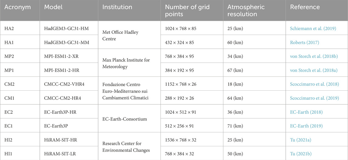
Table 1. Description of the CMIP6-HighResMIP experiments available for historical (1950–2014) and future periods (2015–2050), including the names used in the present study to refer to the experiments. The number of grid points is given in terms of zonal × meridional × vertical resolution.

2.3 Regions of study

The geographical location and meridional extent of South America support diverse climate regimes (Reboita et al., 2010). For effective comparison between models and observational data, five key-subdomains (Figure 1) are selected to represent these climate regimes, defined as: eastern Amazonia (EAZ, 3°N–7°S, 60°W–50°W), northeastern Brazil (NEB, 14°S–4°S, 43°W–37°W), upper Paraguay river basin (UPB, 22.5°S–14°S, 60°W–53°W), upper São Francisco river basin (UFB, 20.5°S–14°S, 50°W–40°W), and the La Plata basin (LPB, 33°S–22.5°S, 60°W–50°W).

Figure 1

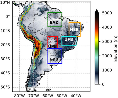
Figure 1. South America topography (shaded, m) and location of the five key-subdomains: eastern Amazonia (EAZ), northeastern Brazil (NEB), upper Paraguay river basin (UPB), upper São Francisco river basin (UFB), and the La Plata basin (LPB).

2.4 Methods

The HighResMIP available simulation period allows us to define the period 1979–2014 as the present climate. The projections are evaluated based on the climatology (annual and seasonal) of this period and the future climate change scenario SSP5-8.5 is represented by the 2015–2050 time slice. This approach ensures a consistent 36-year period for both historical and future climate.

The austral seasons are defined as December-January-February (DJF), March-April-May (MAM), June-July-August (JJA), and September-October-November (SON), allowing for a comprehensive assessment of seasonal variations in precipitation across different climate periods.

All reference data are conservatively remapped to a common resolution grid with 0.25 ° × 0.25 ° of latitude by longitude when the analysis requires data at the same grid, such as the calculation of statistics indices (spatial correlation coefficients, root mean square error, and statistical significance) and bias maps.

2.4.1 Statistical indices

Model evaluation for the present climate compares the simulated seasonal and annual climatologies against reference data by applying some statistical indices, as defined by Wilks (2006). One of these indices is the Pearson’s linear correlation given by Equation 1:

$r_{os}=\frac{\frac{1}{n-1}{\displaystyle \sum _{i=1}^n}\left[\left(o_i-\overline{o}\right)\left(s_i-\overline{s}\right)\right]}{\sqrt{\frac{1}{n-1}{\displaystyle \sum _{i=1}^n}{\left(o_i-\overline{o}\right)}^2}\sqrt{\frac{1}{n-1}{\displaystyle \sum _{i=1}^n}{\left(s_i-\overline{s}\right)}^2}}(1)$

where r_os represents the linear correlation between the observed reference (o) and simulated (s) datasets. For the spatial field correlations, n indicates the total number of grid points in the observed and simulated data.

The average bias was calculated as the difference between the seasonal averages of the simulations and the observed data at each grid point (i) by Equation 2:

$bias=\frac{1}{n}{\displaystyle \sum _{i=1}^n}\left(s_i-o_i\right)(2)$

The root mean square error (RMSE) between the simulation and the observation is calculated as Equation 3:

$RMSE=\sqrt{\frac{1}{n}{\displaystyle \sum _{i=1}^n}{\left(s_i-o_i\right)}^2}(3)$

To evaluate the accuracy of the projections, the Kling-Gupta Efficiency (KGE) index is applied, which was developed by Gupta et al. (2009), and further discussed and applied by Kling et al. (2012). KGE is a global index that considers the linear correlation, bias and variance, given by Equation 4:

$KGE=1-\sqrt{{\left(r_{os}-1\right)}^2+{\left(\frac{{\mathrm{\sigma }}_s}{{\sigma }_o}-1\right)}^2+{\left(\frac{{\mathrm{\mu }}_s}{{\mathrm{\mu }}_o}-1\right)}^2}(4)$

Where r_os represents the correlation between observation and simulation, while σ and μ denote the standard deviation and mean, respectively, for the simulation (σ_s, μ_s) and reference (σ_o, μ_o) datasets. A KGE value greater than −0.41 indicates that the model performs better than using climatology as a predictor for the observed data (Knoben et al., 2019). When KGE approaches 1, it signifies perfect agreement between the model and observations.

The relative changes for the future projections are calculated as the difference between the future and historical climatologies, divided by the historical climatology and expressed as a percentage given by Equation 5:

$trend=\frac{1}{n}{\displaystyle \sum _{i=1}^n}\frac{\left(\overline{fu{t}_i}-\overline{his{t}_i}\right)}{\overline{his{t}_i}}*100\%(5)$

The statistical significance of the spatial correlation for seasonal precipitation is assessed by applying the Student’s t-test, given by Equation 6:

$t=r_{os}*\sqrt{\frac{\left(\nu -2\right)}{\left(1-r_{os}^2\right)}}(6)$

where ν is the degrees of freedom. The statistical significance of future change is determined by testing the difference between the means of two independent samples (Wilks, 2006, given by Equation 7):

$sig=\frac{\left(\overline{fut}-\overline{hist}\right)}{\sqrt{\left({\left[\frac{{\sigma }^2}{n}\right]}_{fut}+{\left[\frac{{\sigma }^2}{n}\right]}_{hist}\right)}}(7)$

The statistical tests are applied to the 95% confidence level.

3 Results

3.1 Defining the reference data for climatology

Considering that the choice of observational reference data influences the evaluation of model simulations (Reboita et al., 2016), the ERA5 and GPCC datasets are first compared with IMERG data. The latter demonstrated good performance when compared with precipitation observed by meteorological stations in mainland China from 2000 to 2018 (Tang et al., 2020), as well as over South America (Dominguez et al., 2024; Prein et al., 2024). These comparisons allow for the assessment of whether the discrepancies between the observational reference and the simulations remain within the range of observationally-based data.

Figure 2 shows the seasonal precipitation climatology (2001–2014) for IMERG data (A) and the biases for ERA5 and GPCC, using IMERG as reference (B; C). Except for JJA, precipitation from the ERA5 reanalysis is higher than in IMERG in the Andes Mountains, exceeding 3 mm day^-1, and in the central Amazon it is up 2–3 mm day^-1 higher. Conversely, ERA5 underestimates IMERG precipitation in the northern part of western Amazonia, with a difference between −1 and −2 mm day^-1. Underestimation also occurs in the central-eastern South America, southern Brazil, and eastern Argentina, where it reaches from −0.5 to −1 mm day^-1 in all seasons. Differences are also noted over the oceans. ERA5 overestimates in approximately 3 mm day^-1 the rainfall of IMERG in tropical latitudes. However, the opposite occurs in the subtropical and extratropical regions of the Atlantic and Pacific Oceans, where ERA5 underestimates IMERG rainfall between −0.5 and −2 mm day^-1. The spatial correlations between ERA5 and IMERG seasonal climatology are high, ranging from 0.89 (JJA) to 0.91 (DJF), with relatively low RMSE, ranging from 1.3 to 1.6 mm day^-1. For all seasons, precipitation amounts from the GPCC are slightly lower (−0.5 and −1 mm day^-1) than IMERG in most regions, with some isolated areas where GPCC overestimates (with some peaks reaching until 2 mm day^-1) the IMERG, such as in the northern Amazon and Andes Mountains, however, the differences exceed 1 mm day^-1 only in a few isolated points. The spatial correlations between GPCC and IMERG for seasonal climatology is very high, ranging from 0.95 (SON) to 0.96 (DJF, MMA, JJA), and RMSE values are lower, ranging from 0.9 to 1.1 mm day^-1.

Figure 2

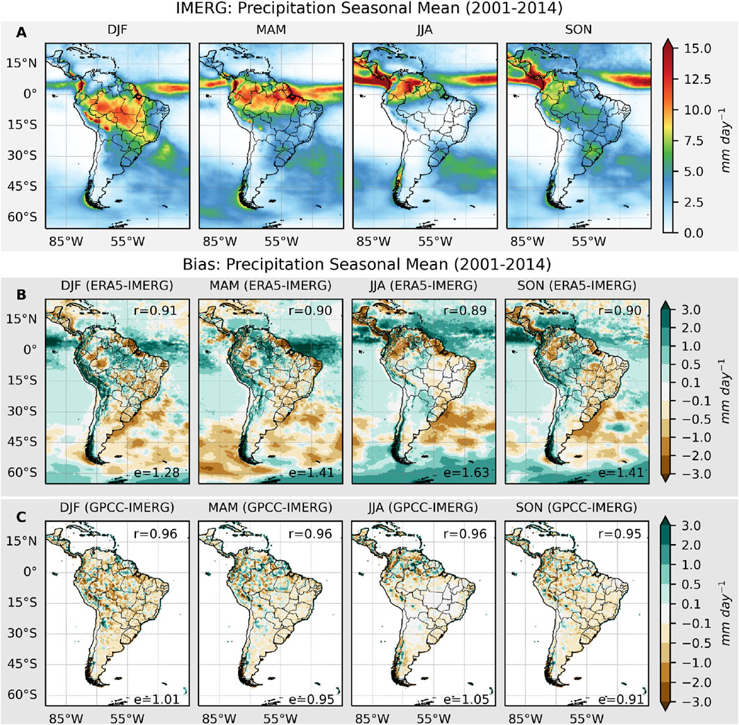
Figure 2. Seasonal climatology (2001–2014) of precipitation (mm day^-1) from observational data: (A) IMERG; Seasonal precipitation biases (mm day^-1) between: (B) ERA5 and IMERG; (C) GPCC and IMERG. The values in the top-right [r] in each panel are the spatial Pearson correlations between data, and in the bottom-right [e] the RMSE.

Considering the spatial patterns and statistical indices (Figure 2), associated with the fact that GPCC and ERA5 cover longer periods, both datasets are used to evaluate the HighResMIP simulations in the subdomains. For the entire South America domain, however, only ERA5 is used, as it includes data over the oceans.

3.2 Simulated precipitation in the present climate

For present climate (1979–2014), the seasonal climatologies of precipitation from ERA5 are shown in Figure 3A, and the bias of the simulated precipitation with respect to the ERA5 reference is also shown in Figures 3B−L. Table 2 synthesizes the statistical indices (spatial correlation coefficients, RMSE, and average bias) between ERA5 and model data for the entire domain of Figure 3. Overall, the simulations are able to capture the annual March of precipitation across the continent (see Supplementary Figure S1), with two distinct peaks, one in austral summer (DJF) over central part of continent, and other in austral winter (JJA) north of the equator. In more detail, the rainy season begins in the austral spring as a band of precipitation extending from the northwest to the center-east of the continent, reaching a peak intensity in austral summer, covering of the most continent (from Amazon basin to central-eastern Brazil), which is a characteristic of the SAMS (Kousky, 1988; Horel et al., 1989; Vera et al., 2006; Reboita et al., 2010; Carvalho and Cavalcanti, 2016). After the peak, precipitation decreases in these regions while increasing in the northwest (north Amazon, Equator, Colombia) and southwest (south Chile) of the continent during austral autumn. In austral winter, most of the continent experiences low precipitation, with some increases over isolated areas: the northwest of the continent and western side of the southern of the Andes Mountains.

Figure 3

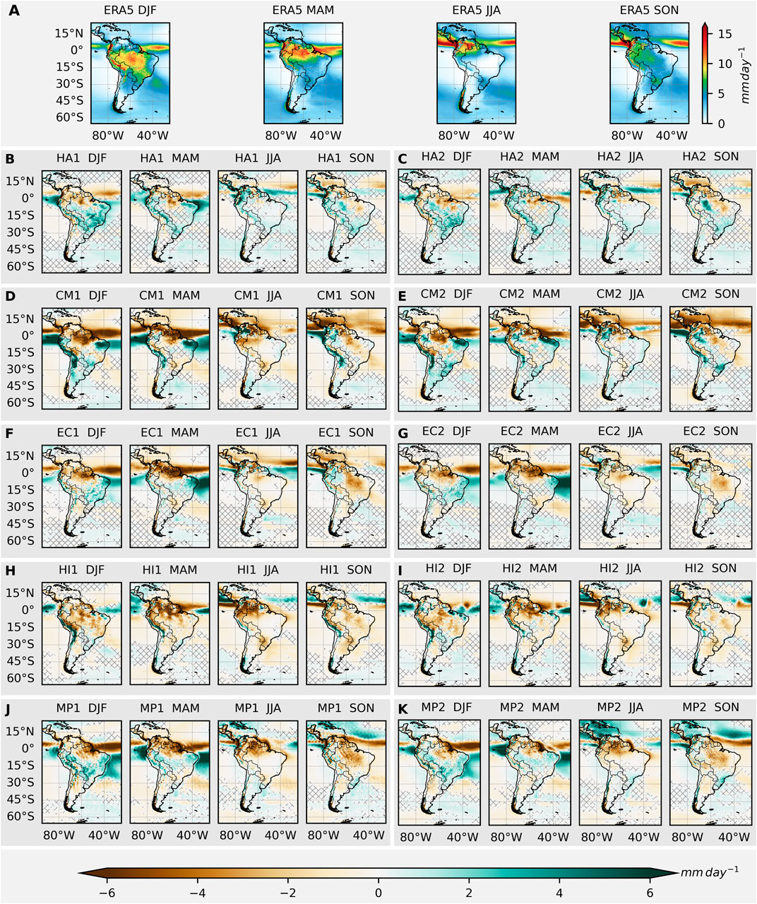
Figure 3. Seasonal precipitation (mm day^-1) climatology (1979–2014) from the observational reference ERA5 reanalysis (A) and seasonal precipitation bias (models minus ERA5; mm day^-1) for the period 1979–2014 of HighResMIP simulations: (B) HA1, (C) HA2, (D) CM1, (E) CM2, (F) EC1, (G) EC2, (H) HI1, (I) HI2, (J) MP1, (K) MP2. Gray hatching represents regions where the differences in means are not statistically significant at the 95% confidence level.

Table 2

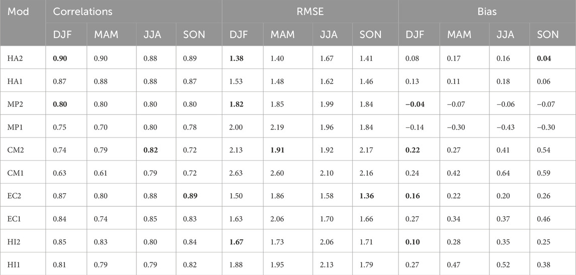
Table 2. Statistical indexes (correlation, RMSE, and bias) obtained from the comparison between simulated and ERA5 reanalysis spatial fields of the seasonal precipitation climatology. The values in bold highlight the best result in each set of models considering the versions in lower and higher resolutions.

The spatial correlations were calculated for the whole domain in Figure 3, which includes different precipitation regimes that will be analyzed further through KGE index for their annual cycles (Section 3.3). The correlations shown in Table 2 indicate that the seasonal cycle of rainfall is very well captured in all simulations since spatial correlations are high, ranging from a minimum of 0.61 to a maximum of 0.90, corresponding to CM1 in austral autumn and HA2 in austral summer, respectively. The lower correlation in CM1 (Figure 3D) may be attributed to misrepresentation of the Intertropical Convergence Zone (ITCZ) south of the equator in the tropical Pacific, which disagrees with both ERA5 and other simulations. This feature is partially improved in CM2 (Figure 3E), reflected in the higher spatial correlation of 0.79 (Table 2). When comparing high and low-resolution simulations, the highest spatial correlations are consistently reached in the high-resolution versions of the HighResMIP coupled models. In austral summer three high-resolution models (HA2, EC2 and HI2) achieve the highest correlations (equal or above 0.85). In austral winter and spring, the highest correlation occurs in both HA2 and EC2, with equal values of 0.88 for winter and 0.89 for spring. It is interesting to note that MP2 achieves a consistent correlation of 0.80 across all seasons, which is higher than that in MP1.

Figure 4 presents the spatial correlation coefficients between simulations and ERA5 dataset considering only the continental grid points. Across all seasons, spatial correlations are consistently higher when only continental grid points are considered (Figure 4) than when the oceans are included (Figure 3), changing from the minimum value 0.61 (CM1, MAM) to 0.78 (CM1, JJA) and maximum from 0.90 (HA2, DJF and MAM) to 0.93 (EC2, DJF). This would indicate that precipitation mechanisms are better solved by HighResMIP GCMs over the continent than oceanic sectors of domain. The errors in ITCZ location and intensity, in both tropical Pacific and Atlantic, may be the main source of simulation errors, which decrease the spatial correlation coefficients in the whole domain. As for all grid points (Table 2) the spatial correlations without ocean (Figure 4) are consistently higher in the fine-resolution compared to coarse simulations for all seasons over the year. The biggest increase in the spatial correlations comes from CM2 and CM1 models, followed by EC2-EC1 and HA2-HA1. Therefore, the greater ability of fine-resolution simulations in capturing small scale processes of precipitation is also reflected in the fact that highest spatial correlation coefficients are reached in DJF and MAM, when large convective activity and SAMS are active over most South America (Vera et al., 2006; Zilli et al., 2024). On other hand, in JJA when rainfall intensity decreases (to less than 50 mm month^-1) over most of the continent the correlations are a little small. This may reflect some difficulty of the models in capturing transient extratropical systems and associated precipitation over the continent, even in fine-resolutions.

Figure 4

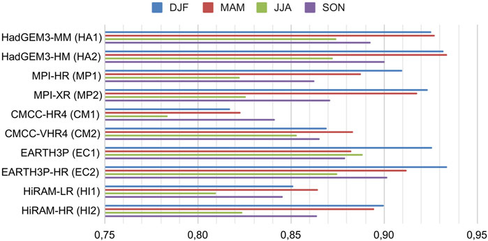
Figure 4. Spatial pattern correlations between historical (1979–2014) precipitation seasonal climatologies simulated by HighResMIP and from ERA5 considering only continental grid points.

The spatial distribution of the seasonal precipitation bias for the HighResMIP simulations is shown in Figure 3, where the gray hatched areas indicate regions with no statistical significance at the 95% confidence level. The RMSE and mean bias (with the best values in bold) for the entire domain are shown in Table 2. A common bias in most simulations is the misrepresentation of the ITCZ location in both the tropical Pacific and Atlantic Oceans. This results from the overestimation of rainfall in its southern branch and an underestimation in its northern sector (Figure 3). Visually, and also considering the RMSE, most of the higher-resolution simulations improve this feature, resulting in smaller RMSEs. This suggests the better ability of high-resolution in capturing the more intense and weak cores of precipitation, as previously noted for the ITCZ. Of particular interest in Figure 3 is the improvement in simulating rainfall over the Andes Mountains, with fine-resolution reducing the biases, mainly in austral summer and autumn. This feature also helps explain the higher spatial correlations obtained by high-resolution models over the continent (Figure 4). With rare exceptions (H2 and CM2, both in SON), precipitation biases (values in Table 2) also decrease in fine-resolution simulations. Examining Figure 3, it is noted that the decrease of both RMSE and biases is achieved by improving the location and intensity of rainfall in ITCZ in their high-resolution versions, mainly in austral summer and autumn (Figure 3). Additionally, the areas where the simulated means are not significantly different from the reference data (gray hatched regions, Figure 3) increase in higher-resolution simulations.

For most seasons of the year, the simulations present a dry bias in the equatorial Amazon (associated with the misrepresentation of the ITCZ location), which decreases with the increase in model resolution (Figure 3). A similar improvement was already identified by de Souza Custodio et al. (2017) when comparing HadGEM1 in three different horizontal resolutions (∼120, 90 and 60 km) over South America. Except for the HiRAM model (HI1 and HI2), in DJF all other experiments have a wet bias in the center-eastern sector of the continent, in both high and low-resolutions. For MAM and SON, CM1 presents a dry bias in southern Brazil, which invert its signal in CM2 (Figures 3D,E). In the central-east of the continent in SON, high-resolution simulations reduce the dry bias, while an increase in the wet bias occurs in the western Brazilian Amazon.

Figure 5 presents the annual climatology of evapotranspiration from ERA5 and the ensembles of low (Ens1, Figure 5B) and high-resolution (Ens2, Figure 5C) simulations, along with their respective biases (Figures 5D,E respectively). The ensembles adequately reproduce the evapotranspiration pattern depicted by ERA5, which shows higher values over the northwestern Amazon and lower values over northeastern Brazil and from south to northwestern Argentina. Over the ocean, notable features include high evaporation in the Brazil-Malvinas confluence zone and the tropical Atlantic ocean. The ability to capture the ERA5 pattern is reflected in high spatial correlations of 0.96 for Ens1 and 0.97 for Ens2. The bias maps (Figures 5D,E) reveal subtle differences between high and low-resolution simulations. For instance, Ens2 reduces the dry bias observed in the Ens1 along the north continental coast, but slightly increases the wet bias over the northwest of Amazon basin.

Figure 5

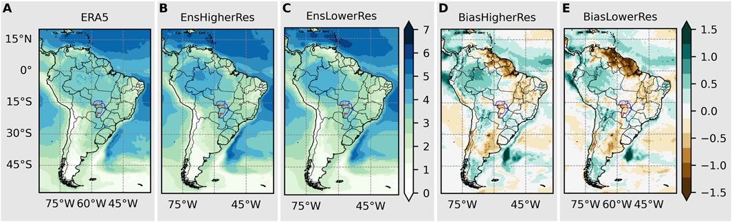
Figure 5. Annual climatology (1979–2014) of evapotranspiration (mm day^-1) from: (A) observational reference ERA5 reanalysis; (B) Ens2 - ensemble mean of high-resolution simulations - (HA2, MP2, CM2, EC2, HI2); (C) Ens1 - ensemble mean of low-resolution simulations (HA1, MP1, CM1, EC1, HI1); (D) Ens2 bias in relation toERA5; (E) Ens1 bias in relation to ERA5.

3.3 Simulated annual cycle in key-regions

Figure 6 shows the mean (1979–2014) annual cycles of precipitation and evapotranspiration from simulations and reference data (ERA5 and GPCC) for each key-subregion indicated in Figure 1. According to Figure 6, the selected key-regions have different precipitation regimes. UPB and UFB are characterized by the rainy season from October to March and dry season from April to September. In these regions, the simulated precipitation from March to October closely matches the ERA5 and GPCC data, with minor biases, while the bias increases differently in each region in January-February. For UPB, simulations overestimate rainfall from January to February (Figure 6A), while the decrease in rainfall shown in the reference data for UFB is only captured by CM1, CM2, HI1 and HI2.

Figure 6

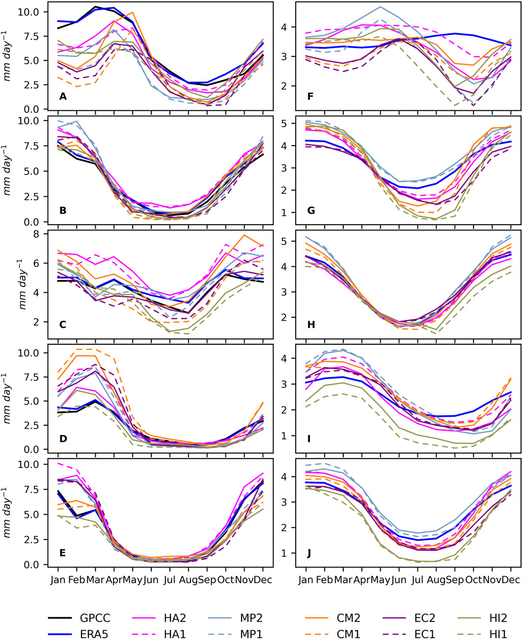
Figure 6. Mean annual cycle (1979–2014) in key-regions of precipitation (mm day^-1) from reference data (ERA5 and GPCC) and simulations (legend): (A) EAZ; (B) UPB; (C) LPB; (D) NEB; (E) UFB; evapotranspiration (mm/day) from reference data (ERA5) and simulations (legend): (F) EAZ; (G) UPB; (H) LPB; (I) NEB; (J) UFB.

The greatest spread between simulations and reference data occurs throughout the year in the LPB and from January to May in NEB and EAZ (Figure 6). In the LPB, HA1 and HA2 overestimate precipitation in all months of the year, while in the CMCC model the rainfall biases depend on the resolution (overestimation in CM1 and underestimation in CM2). All simulations in EAZ underestimate rainfall over the year, but the biases are larger during the rainy season (January to May), while almost the opposite occurs in NEB except in HI1.

The evapotranspiration annual cycle (Figures 6F–I) follows that of precipitation in the UPB, UFB, and NDE regions, with maxima and minima occurring during the wet and dry seasons, respectively. This pattern, although with differences in amplitude, is captured by all simulations, with minor discrepancies between the low and high-resolution models, as already indicated by the bias maps (Figures 5D,E). As shown in Figure 6, the annual cycle of evapotranspiration differs from that of precipitation in the EAZ and LPB regions, which is a feature also reported in the literature (da Rocha et al., 2012; Drumond et al., 2024). In ERA5 the evapotranspiration over EAZ remains nearly constant from December to June (∼3.5 mm day^-1), with a slight increase from July to November (∼4.0 mm day^-1). This behavior aligns with flux measurements in towers in the region (da Rocha et al., 2012), but is rarely reproduced by climate simulations over the Amazon (Teodoro et al., 2021; Baker et al., 2021; da Rocha et al., 2012). In both high and low-resolution simulations the annual cycles of evapotranspiration in EAZ have a very large amplitude and follow approximately the annual cycle of rainfall (Figure 6A), having maximum in the rainy season and minimum in the dry season (Figure 6F). Therefore, the simulated annual cycles are entirely out of phase compared to ERA5, since they replicate the annual cycle of precipitation instead of accurately representing the evapotranspiration physical processes. This indicates that previously reported simulations challenge in relation to the near surface budget in the Amazon basin (da Rocha et al., 2012; Baker et al., 2021) remain in high-resolution HighResMIP GCMs. In the LPB region, the annual cycle of evapotranspiration in ERA5 peaks in summer and reaches its minimum in winter, which is out of phase with precipitation (Figure 6C). However, this pattern is adequately captured by the simulations, with only minor differences between high and low-resolution models (Figure 6H).

In order to quantify the differences between high and low-resolution simulations in reproducing the spatial distribution of the precipitation and evapotranspiration annual cycles, the KGE index is shown for the key-regions in Figure 7. Arrows in Figure 7 point to the model resolution with the highest KGE value, which indicates superior performance of low or high-resolution versions across different regions. Regarding precipitation, with few exceptions (e.g., UPB) KGE values are consistently higher when simulations are compared with GPCC (Figure 7A) rather than with ERA5 (Figure 7B), generally favoring high-resolution simulations. In particular, NEB, LPB and EAZ exhibit the greatest improvements in representing the annual rainfall cycle in high-resolutions, with marked increases in KGE (sometimes shifting from negative to positive values) across most models. When comparing all regions, UPB and UFB present the higher KGE values (above 0.6), indicating a greater ability of models to represent annual rainfall cycles and reduced sensitivity to model resolution, as reflected by the similar KGEs for both resolutions. For evapotranspiration (Figure 7C), high KGE values (above 0.5) indicate the ability of the simulations to reproduce the ERA5 annual cycles in the UFB and LPB regions. Regarding resolution, a subtle improvement is observed in the high-resolution models for capturing the annual cycle of evapotranspiration in most regions, except in the NEB, where this improvement is only seen in HA2. The difficulty of the simulations in capturing the observed annual cycle of evapotranspiration in the EAZ is evident from the KGE, which shows significantly negative values.

Figure 7

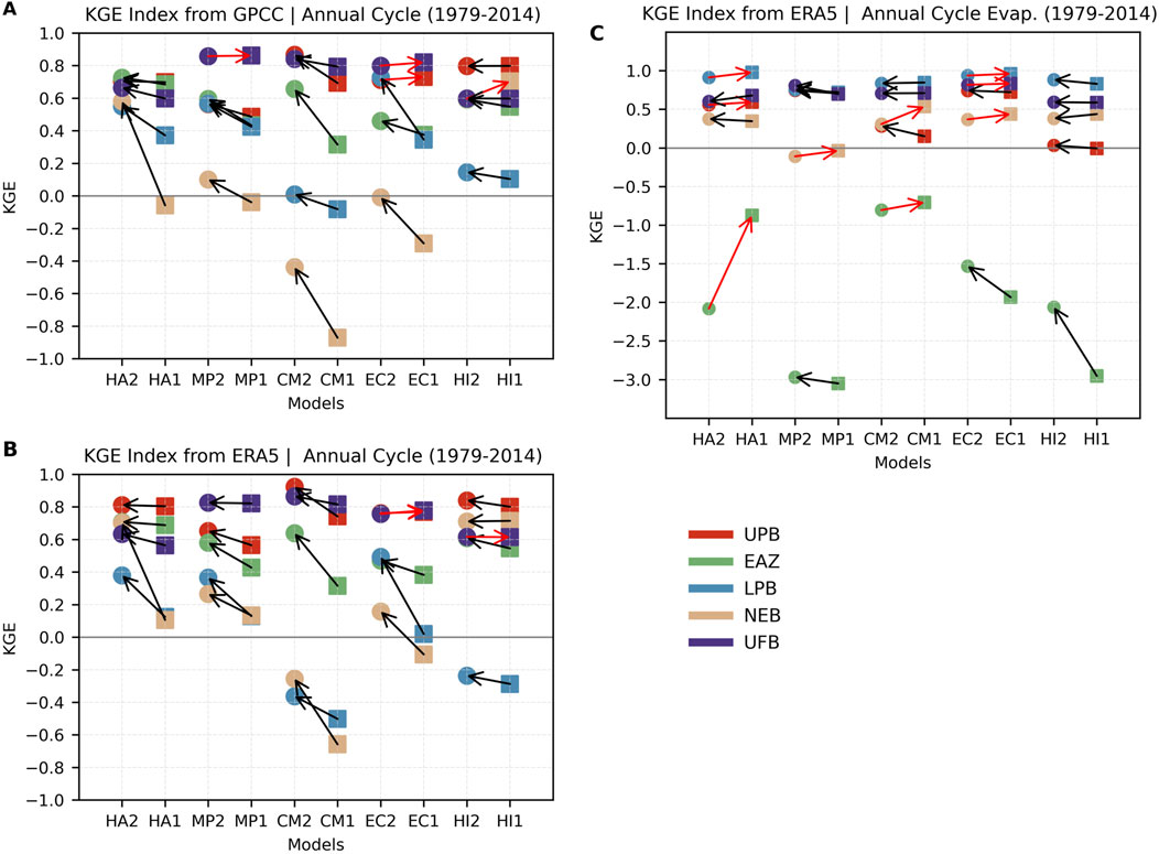
Figure 7. KGE index for the mean annual cycle (1979–2014) in each subdomain (color-coded) for simulations in high (circles) and low (squares) resolutions, considering: (A) precipitation, with GPCC as reference; (B) precipitation, with ERA5 as reference; (C) evapotranspiration, with as reference ERA5. The arrows point towards the high values of KGE in function of model resolution.

3.4 Future projections in SSP5-8.5 scenario

3.4.1 Changes in seasonal rainfall

Considering that the main features of observed climatology are well captured by the models in the historical period, future changes are analyzed as the difference between future SSP5.8.5 scenario (2015–2050) and present climate (1979–2014) periods. Figure 8 presents the projected seasonal relative changes of precipitation.

Figure 8

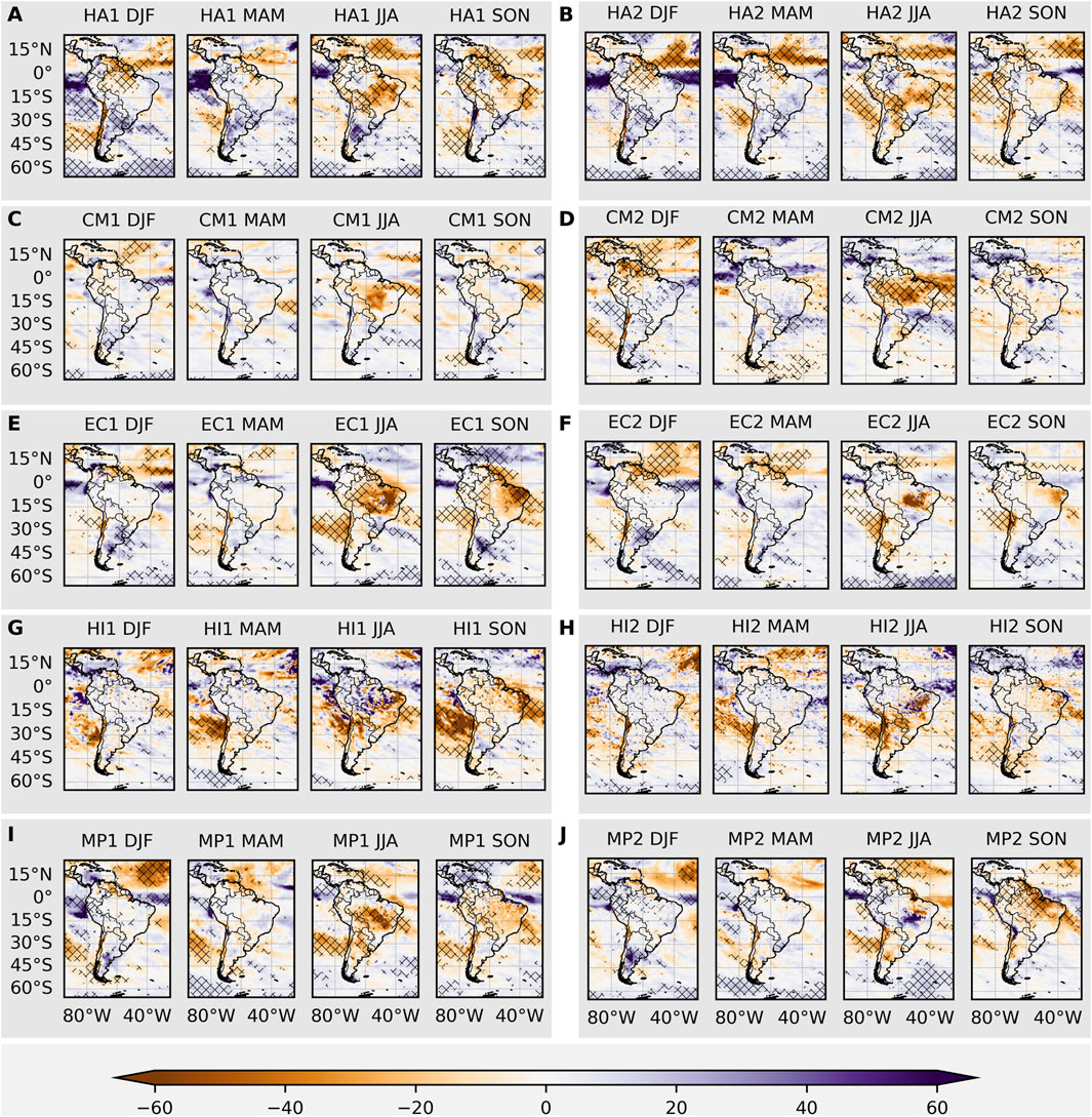
Figure 8. Relative (%) rainfall future projections (2015–2050) for seasonal climatology from: (A) HA1, (B) HA2, (C) CM1, (D) CM2, (E) EC1, (F) EC2, (G) HI1, (H) HI2, (I) MP1, (J) MP2. Hatching represents regions where the differences in means are statistically significant at the 95% confidence level.

The relative changes in precipitation are most prominent in austral spring and winter over the continent, as well as over the oceans throughout all seasons (Figure 8). Notably, the projected changes across different models show a common strong signal of a decrease in precipitation over the continental sector of SAMS and north-northeast coast of Brazil during the austral spring, extending from northwest to southeast of South America (Figure 8), as well over the central-northeast parts of Brazil during winter. In this season, there is a widespread reduction in precipitation during winter across northern South America, Central America, and the Amazon basin. These areas of decreased precipitation align with the changes projected by CMIP6 models depicted by Ortega et al. (2021). Their findings indicate larger magnitudes of change compared to the mid-century HighResMIP time slice used in this study. In austral summer and autumn the greater relative changes in rainfall occur in the regions of Pacific and Atlantic ITCZ. There is also a projected increase in precipitation across southern Brazil, extending into northeastern Argentina, and crossing Uruguay and Paraguay. Additionally, a reversal ośf the precipitation change signal is noted in some models, as near the coast southeast of Brazil and over subtropical Pacific Ocean (Figure 8).

3.4.2 Water resources trends

From a climactic point of view, a measure of WR on the surface can be obtained as the difference between precipitation (P) and evapotranspiration (ET), i.e., (P minus ET), as discussed by Llopart et al. (2019). The annual future relative changes in WR for each projection are shown in Figure 9, while changes in ET and P are presented in Supplementary Figure S3, which provides additional insight into the spatial patterns of these variables (Supplementary Material). For comparison with the literature, the ensemble means are provided in Supplementary Figure S2.

Figure 9

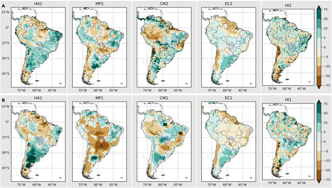
Figure 9. Relative (%) annual future changes in the water resources projected by HighResMIP models in (A) high and (B) low-resolutions.

According to Figure 9, high-resolution projections agree with the mid-century band of positive WR change, which crosses the continent starting in the northeast of Brazil and heading towards the southwest of the continent. This change signal is more intense and defined in some models (HA2, CM2 and EC2) and less in others (MP2 and HI2). In particular, HI2 presents a very noisy pattern of change, which intersperses positive and negative cores without a clear pattern. Another important signal is the region of decreasing WR occupying most of the Amazon basin in high-resolution projections (Figure 9). The described pattern of future changes in WR aligns with the spatial distribution of changes in P and ET shown in Supplementary Figure S3.

Most models indicate that in EAZ, both P and ET decrease (Supplementary Figure S3). In UPB, the reduction in ET and P is a predominant pattern, except in CM2 and EC2 and HI1 and HI2 that exhibit an increase in P only. In LPB, both ET and P tend to increase, except in HI1 and HI2. In NEB, the general pattern is a decrease in ET and an increase in P, although HA2 presents an opposite signal for ET. In UFB, both ET and P increase, but in lower-resolution projections, P tends to decrease, while the signal of ET increase is more consistent in higher-resolution versions. The described patterns of future changes in WR becomes clearer when considering these regional characteristics of ET and P changes. These patterns suggest that higher-resolution models generally present fewer areas with ET reduction, as also noted in Supplementary Figure S3.

The described pattern of future changes in WR are not very evident in low-resolution projections, with larger divergence between them. For example, WR is projected to increase in the center-north of Argentina until south Brazil in HA1 and EC1, but not in MP1, CM1 and HI1 (Figure 9). Similarly, the extensive area of WR decline over the Amazon basin is clearly captured in high-resolution projections, but it is less well-defined in low-resolution simulations.

In the ensemble means (Supplementary Figure S2, in Supplementary Material), the differences in the patterns projected for water resources as a function of resolution are clearer. The northeast-southwest band of the future increases in water resources, crossing the continent from northeast Brazil to central Argentina, as well as the projected decrease over Amazon basin are better defined in high than low-resolution (Supplementary Figure S2). This pattern is similar to the ones found by Llopart et al. (2019) using an ensemble of RCM projections. Some differences exist in the intensity of the changes, since Llopart et al. (2019) investigated the end century (2070–2099) and obtained stronger relative changes (reaching until 70%), while Figure 9 is showing weaker changes (maximum 50%) at the mid-century. In the ensemble means at low-resolution the northeast-southwest corridor of increasing WR is not evident (Supplementary Figure S2) as obtained also by Llopart et al. (2019) for coarser resolution GCMs from CMIP5. As argued by Llopart et al. (2019), model resolution plays a crucial role in projecting changes in surface moisture availability since it can better solve the physical processes associated with near surface variables, such as precipitation and evapotranspiration. This improvement occurs, for example, in HighResMIP seasonal precipitation patterns mostly over the continent (Figure 4).

For austral summer and winter, Figures 10, 11 present the time series of the anomalies (calculated with respect to the 1979–2014 period) of precipitation, evapotranspiration, and water resource for the key regions. The time series are 14-year running mean anomalies following the methodology used by Coppola and Giorgi (2010) and Llopart et al. (2019), adjusted here for a smaller window (14 years) due to the series being 76 years long, rather than 20 years running mean used for 100 years period in the reported studies. The statistical significant (at 95% confidence level) trends from 2015–2050 are shown in each panel.

Figure 10

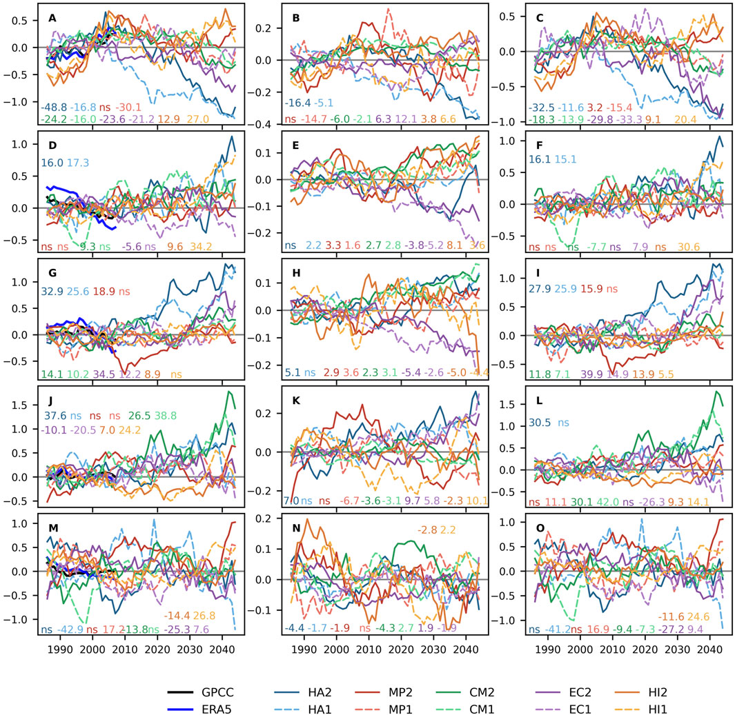
Figure 10. High (continuous lines) and low (dashed lines) resolution simulated time series (1979–2050) for austral summer (DJF) of precipitation (A,D,G,J,M), evapotranspiration (B,E, H,K,N), and water resource (C,F,I,L,O) anomalies (mm day^-1) smoothed using an running mean with a 14-years window for the regions: (A,B and C) EAZ, (D,E and F) UPB, (G,H and I) LPB, (J,K, L) NEB, (M,N,O) UFB. For 1979–2014 the precipitation from GPCP and ERA5 are also included in (A,D,G,J,M) panels. The numbers with the same curve colors for each model represent the statistically significant (at 95% confidence level) linear trend (x10⁻³ mm d^-1 y^-1) projections (2015–2050), with ‘ns’ indicating trends that did not reach this significance level.

Figure 11

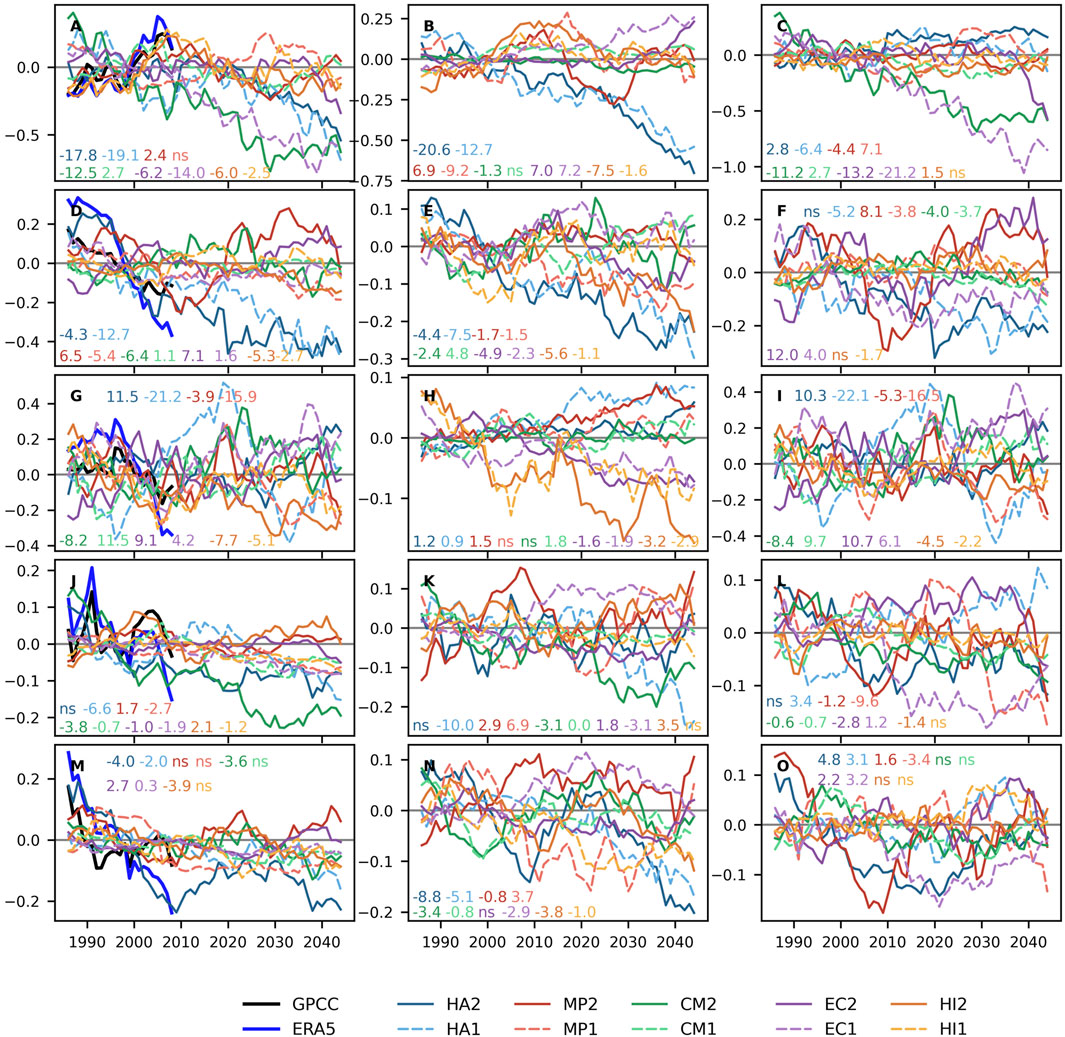
Figure 11. High (continuous lines) and low (dashed lines) resolution simulated time series (1979–2050) for austral winter (JJA) of precipitation (A,D,G,J,M), evapotranspiration (B,E,H,K,N), and water resource (C,F,I,L,O) anomalies (mm day^-1) smoothed using an running mean with a 14-years window for the regions: (A,B and C) EAZ, (D,E and F) UPB, (G,H and I) LPB, (J,K,L) NEB, (M,N,O) UFB. For 1979–2014 the precipitation from GPCP and ERA5 are also included in (A,D,G,J,M) panels. The numbers with the same curve colors for each model represent the statistically significant (at 95% confidence level) linear trend (x10⁻³ mm d^-1 y^-1) projections (2015–2050), with ‘ns’ indicating trends that did not reach this significance level.

For both austral summer (Figure 10) and winter (Figure 11), together with a long term trend, the time series in each key region highlight the existence of low frequency (decadal or longer) variability of precipitation and evapotranspiration. Another interesting aspect is that for some variables and regions the low frequency variability is not always in the phase between low and high-resolution simulations.

In most projections, rainfall will decrease in EAZ with consequent negative trends in WR in austral summer (Figure 10C). This occurs both in projections that also indicate a negative evapotranspiration trend (Figure 10B; HA1, HA2, MP2, CM2, CM1) and in those with a positive or non-significant trend of ET (EC1, EC2, HI1, HI2), since negative trend of precipitation is more accentuated. For JJA (Figure 11C), WR decreasing is also a predominant signal in most projections mainly associated with stronger negative trends in rainfall, except in HA1 that projects increasing water availability due to stronger decreases of ET. The predominance of the negative trend of rainfall controlling the future decreases in water availability in the EAZ region is similar to that found by Llopart et al. (2019); Llopart et al. (2020) for similar regions.

In the central part of the continent, for UPB and LPB regions most projections indicate statistically significant positive trend in WR in austral summer (Figures 10F-I). This trend is mainly due to the increase in precipitation, which exceeds the positive trend in evapotranspiration. The exceptions are EC1-EC2 and HI1-HI2, where the increase in water availability occurs associated with the increase of rainfall and decrease of evapotranspiration (Figures 10F,I). On the other hand, in JJA a larger number of statistically significant projections are indicating a future decrease of water availability in UPB and LPB associated with the stronger decrease of rainfall than evapotranspiration (Figures 11F−I)

The WR trend mechanism in DJF over the LPB (increase of WR due to increase of P and ET) is similar to that obtained from RCM projections and differs from the mechanism in GCM projections (increases WR due to increase of P and decreases ET) analyzed by Llopart et al. (2019), Llopart et al. (2020). As all GCMs used here have higher resolution than GCMs in Llopart et al. (2019), Llopart et al. (2020), the compatibility of mechanisms of HighResMIP with RCMs demonstrate the role of model resolution in solving water availability at surface.

For tropical region NEB, there is a predominance of projections showing greater water availability during summer as a consequence of increasing rainfall and decreasing of evapotranspiration or stronger increase of rainfall than evapotranspiration (Figures 10J–L). In NEB, the predominance of a future with more water availability as a function of positive trend of rainfall and negative ones of evapotranspiration is similar to that found by Llopart et al. (2019) for the end of 21 century. On the other hand, in the UFB predominates future water availability decreasing due to the strong negative change of rainfall (Figures 10M–O).

During austral winter, the projections indicated a predominance of negative change in WR in NEB as a function of the projected decrease in precipitation and increased evapotranspiration (Figures 11J–L). This signal differs from Llopart et al. (2019) in that obtained WR increased at the end of the century in a similar region even with a negative rainfall trend, but decreased in evapotranspiration. For the UPB region, a great number of trends indicate a future decrease of rainfall, but this change is weaker than the negative trend in ET resulting in a positive trend of water availability (Figures 11M–O).

4 Discussion

This study evaluated five coupled GCMs from the HighResMIP-CMIP6 experiment to assess the impact of increasing horizontal resolution (∼70 km vs. ∼25 km) on the representation of present climate and projections of future changes in precipitation, evapotranspiration, and water availability over South America. The analysis covered historical (1979–2014) and future (2015–2050) periods under the SSP5-8.5 scenario. High-resolution simulations improved the representation of seasonal precipitation, particularly over land, capturing the austral summer peak in central South America and winter peak north of the equator. These models better resolve small-scale precipitation mechanisms, especially during austral summer-autumn, but persistent errors in ITCZ position and intensity remain, affecting spatial correlations when adjacent oceans are included. For annual precipitation cycles, high-resolution models show a consistent improvement in NEB, LPB, and EAZ, while in UPB and UFB, both resolutions adequately capture observations. A notable challenge remains in simulating evapotranspiration over the Amazon, particularly in EAZ, where neither resolution reproduces its observed annual cycle. Future projections indicate a more intense dry season, with rainfall reductions exceeding 30% in central South America. In contrast, increased precipitation is projected in austral summer-autumn south of 25°S, including LPB. However, precipitation projections depend on model resolution, with high-resolution models showing different spatial patterns. Regarding water availability, high-resolution models consistently project a southwest-northeast band of wetter conditions from Argentina to northeastern Brazil and a drier Amazon basin. These patterns align with RCM projections nested in CMIP5-GCMs, reinforcing the role of resolution in future water resource assessments. In summary, high-resolution models improve the representation of precipitation and evapotranspiration, particularly over land, but challenges remain in simulating ITCZ rainfall and Amazon evapotranspiration. Future work should explore soil-atmosphere interactions and the impact of resolution on interannual variability, such as ENSO-related rainfall changes over South America.

Data availability statement

Publicly available datasets were analyzed in this study. This data can be found here: HighResMip: https://highresmip.org/data/; https://psl.noaa.gov/data/gridded/data.gpcc.html; https://climatedataguide.ucar.edu/climate-data/gpm-global-precipitation-measurement-mission; https://cds.climate.copernicus.eu/datasets/reanalysis-era5-single-levels?tab=overview; https://aims2.llnl.gov/metagrid/search/?project=CMIP6.

Author contributions

NS: Conceptualization, Data curation, Formal Analysis, Investigation, Methodology, Project administration, Software, Visualization, Writing – original draft. RR: Conceptualization, Funding acquisition, Project administration, Supervision, Writing – review and editing. AN: Formal Analysis, Supervision, Writing – review and editing.

Funding

The author(s) declare that financial support was received for the research and/or publication of this article. The authors would like to thank the Instituto Federal de Educação Ciência e Tecnologia de Mato Grosso do Sul, Conselho Nacional de Desenvolvimento Científico e Tecnológico (CNPq; Grants #401868/2022-2, #305349/2022-8), and Coordenação de Aperfeiçoamento de Pessoal de Nível Superior–Brasil (CAPES) - Financing Code 001 and FAPESP (Grants #2022/05476-2).

Acknowledgments

The authors would like to thank the Global Precipitation Climatology Centre (GPCC) data provided by the NOAA PSL, Boulder, Colorado, United States, from their website at https://psl.noaa.gov.

Conflict of interest

The authors declare that the research was conducted in the absence of any commercial or financial relationships that could be construed as a potential conflict of interest.

Generative AI statement

The author(s) declare that Generative AI was used in the creation of this manuscript. Chatgpt 4.0 was used to correct and edit grammar issues in the English language.

Publisher’s note

All claims expressed in this article are solely those of the authors and do not necessarily represent those of their affiliated organizations, or those of the publisher, the editors and the reviewers. Any product that may be evaluated in this article, or claim that may be made by its manufacturer, is not guaranteed or endorsed by the publisher.

Supplementary material

The Supplementary Material for this article can be found online at: https://www.frontiersin.org/articles/10.3389/feart.2025.1537081/full#supplementary-material

References

Ajibola, F. O., Zhou, B., Gnitou, G. T., and Onyejuruwa, A. (2020). Evaluation of the performance of CMIP6 HighResMIP on west african precipitation. Atmosphere 11, 1053. doi:10.3390/atmos11101053

CrossRef Full Text | Google Scholar

Asong, Z. E., Razavi, S., Wheater, H. S., and Wong, J. S. (2017). Evaluation of integrated multisatellite Retrievals for GPM (IMERG) over southern Canada against ground precipitation observations: a preliminary assessment. J. Hydrometeorol. 18, 1033–1050. doi:10.1175/JHM-D-16-0187.1

CrossRef Full Text | Google Scholar

Avila-Diaz, A., Abrahão, G., Justino, F., Torres, R., and Wilson, A. (2020). Extreme climate indices in Brazil: evaluation of downscaled earth system models at high horizontal resolution. Clim. Dyn. 54, 5065–5088. doi:10.1007/s00382-020-05272-9

CrossRef Full Text | Google Scholar

Avila-Diaz, A., Torres, R. R., Zuluaga, C. F., Cerón, W. L., Oliveira, L., Benezoli, V., et al. (2023). Current and future climate extremes over Latin america and caribbean: assessing earth system models from high resolution model intercomparison project (HighResMIP). Earth Syst. Environ. 7, 99–130. doi:10.1007/s41748-022-00337-7

PubMed Abstract | CrossRef Full Text | Google Scholar

Baker, J. C. A., de Souza, D. C., Kubota, P. Y., Buermann, W., Coelho, C. A. S., Andrews, M. B., et al. (2021). An assessment of land–atmosphere interactions over SouthSouth America using satellites, reanalysis, and two global climate models. J. Hydrometeorol. 22, 905–922. doi:10.1175/JHM-D-20-0132.1

CrossRef Full Text | Google Scholar

Bazzanela, A. C., Dereczynski, C. P., Luiz-Silva, W., and Regoto, P. (2023). Performance of CMIP6 models over SouthSouth America. Clim. Dyn. 62, 1501–1516. doi:10.1007/s00382-023-06979-1

CrossRef Full Text | Google Scholar

Bock, L., Lauer, A., Schlund, M., Barreiro, M., Bellouin, N., Jones, C., et al. (2020). Quantifying progress across different CMIP phases with the ESMValTool. J. Geophys. Res. Atmos. 125. doi:10.1029/2019JD032321

CrossRef Full Text | Google Scholar

Carril, A. F., Cavalcanti, I. F. A., Menéndez, C. G., Sörensson, A. A., López-Franca, N., Rivera, J. A., et al. (2016). Extreme events in the la Plata basin: a retrospective analysis of what we have learned during claris-lpb project. Clim. Res. 68, 95–116. doi:10.3354/cr01374

CrossRef Full Text | Google Scholar

Carvalho, L. M. V., and Cavalcanti, I. F. A. (2016). The South American monsoon system (SAMS), in The monsoons and climate change. Editors L. de Carvalho, and C. Jones (Cham: Springer Climate. Springer). doi:10.1007/978-3-319-21650-8_6

CrossRef Full Text | Google Scholar

Clarke, B., Otto, F. E. L., Stuart-Smith, R. F., and Harrington, L. J. (2022). Extreme weather impacts of climate change: an attribution perspective. Environ. Res. Clim. 1, 012001. doi:10.1088/2752-5295/ac6e7d

CrossRef Full Text | Google Scholar

Coppola, E., and Giorgi, F. (2010). An assessment of temperature and precipitation change projections over Italy from recent global and regional climate model simulations. Int. J. Climatol. 30, 11–32. doi:10.1002/joc.1867

CrossRef Full Text | Google Scholar

da Rocha, R. P., Cuadra, S., Reboita, M., Kruger, L., Ambrizzi, T., and Krusche, N. (2012). Effects of RegCM3 parameterizations on simulated rainy season over South America. Clim. Res. 52, 253–265. doi:10.3354/cr01065

CrossRef Full Text | Google Scholar

de Souza Custodio, M., da Rocha, R. P., Ambrizzi, T., Vidale, P. L., and Demory, M. (2017). Impact of increased horizontal resolution in coupled and atmosphere-only models of the HadGEM1 family upon the climate patterns of South America. Clim. Dyn. 48 (9-10), 3341–3364. doi:10.1007/s00382-016-3271-8

CrossRef Full Text | Google Scholar

Dominguez, F., Rasmussen, R., Liu, C., Ikeda, K., Prein, A., Varble, A., et al. (2024). Advancing South American water and climate science through multidecadal convection-permitting modeling. Bull. American Meteorological Soc. 105 (1), E32–E44. doi:10.1175/BAMS-D-22-0226.1

CrossRef Full Text | Google Scholar

Drumond, A., de Oliveira, M., Reboita, M. S., Stojanovic, M., Nunes, A. M. P., and da Rocha, R. P. (2024). Moisture transport during anomalous climate events in the La Plata Basin. Atmosphere 15, 876. doi:10.3390/atmos15080876

CrossRef Full Text | Google Scholar

Ec-Earth, C. (2018). EC-Earth-Consortium EC-Earth3P-HR model output prepared for CMIP6 HighResMIP hist-1950. Earth Syst. grid Fed. doi:10.22033/ESGF/CMIP6.4683

CrossRef Full Text | Google Scholar

Ec-Earth, C. (2019). EC-Earth-Consortium EC-Earth3P model output prepared for CMIP6 HighResMIP hist-1950. Earth Syst. Grid Fed. doi:10.22033/ESGF/CMIP6.4682

CrossRef Full Text | Google Scholar

Eyring, V., Bony, S., Meehl, G. A., Senior, C. A., Stevens, B., Stouffer, R. J., et al. (2016). Overview of the coupled model intercomparison project phase 6 (CMIP6) experimental design and organization. Geosci. Model Dev. 9 (5), 1937–1958. doi:10.5194/gmd-9-1937-2016

CrossRef Full Text | Google Scholar

Firpo, M. Â. F., Guimarães, B. D. S., Dantas, L. G., Silva, M. G. B. D., Alves, L. M., Chadwick, R., et al. (2022). Assessment of CMIP6 models’ performance in simulating present-day climate in Brazil. Front. Clim. 4, 948499. doi:10.3389/fclim.2022.948499

CrossRef Full Text | Google Scholar

Giorgi, F., Coppola, E., Jacob, D. J., Teichmann, C., Omar, S. A., Ashfaq, M., et al. (2021). The cordex-core exp-i initiative: Description and highlight results from the initial analysis. Bull. American Meteorological Soc. 103, E293–E310. doi:10.1175/bams-d-21-0119.1

CrossRef Full Text | Google Scholar

Gupta, H. V., Kling, H., Yilmaz, K. K., and Martinez, G. F. (2009). Decomposition of the mean squared error and NSE performance criteria: implications for improving hydrological modelling. J. Hydrol. 377 (1-2), 80–91. doi:10.1016/j.jhydrol.2009.08.003

CrossRef Full Text | Google Scholar

Haarsma, R. J., Roberts, M. J., Vidale, P. L., Senior, C. A., Bellucci, A., Bao, Q., et al. (2016). High resolution model intercomparison project (HighResMIP v1.0) for CMIP6. Geosci. model Dev. 9, 4185–4208. doi:10.5194/gmd-9-4185-2016

CrossRef Full Text | Google Scholar

Hersbach, H., Bell, B., Berrisford, P., Hirahara, S., Horányi, A., Muñoz-Sabater, J., et al. (2020). The ERA5 global reanalysis. Q. J. R. Meteorological Soc. 146 (730), 1999–2049. doi:10.1002/qj.3803

CrossRef Full Text | Google Scholar

Horel, J. D., Hahmann, A. N., and Geisler, J. E. (1989). An investigation of the annual cycle of convective activity over the tropical americas. J. Clim. 2, 1388–1403. doi:10.1175/1520-0442(1989)002<1388:aiotac>2.0.co;2

CrossRef Full Text | Google Scholar

Hoyos, N., Escobar, J., Restrepo, J. C., Arango, A. M., and Ortíz, J. C. (2013). Impact of the 2010–2011 La Niña phenomenon in Colombia, South America: the human toll of an extreme weather event. Appl. Geogr. 39, 16–25. doi:10.1016/j.apgeog.2012.11.018

CrossRef Full Text | Google Scholar

Huffman, G. J., Bolvin, D. T., Braithwaite, D., Hsu, K., Joyce, R., Kidd, C., et al. (2019). Algorithm theoretical basis document (ATBD) version 5.2 for the NASA global precipitation measurement (GPM) integrated multi-satellite Retrievals for GPM (I-MERG). NASA GPM. Available online at: https://gpm.nasa.gov/sites/default/files/document_files/IMERG_ATBD_V5.2_0.pdf.

Google Scholar

Ito, R., Nakaegawa, T., and Takayabu, I. (2020). Comparison of regional characteristics of land precipitation climatology projected by an MRI-AGCM multi-cumulus scheme and multi-SST ensemble with CMIP5 multimodel ensemble projections. Prog. earth Planet. Sci. 77 (7), 77–20. doi:10.1186/s40645-020-00394-4

CrossRef Full Text | Google Scholar

Junk, W. J., and Cunha, C. N. D. (2005). Pantanal: a large south american wetland at a crossroads. Ecol. Eng. 24, 391–401. doi:10.1016/j.ecoleng.2004.11.012

CrossRef Full Text | Google Scholar

Kling, H., Fuchs, M., and Paulin, M. (2012). Runoff conditions in the upper Danube basin under an ensemble of climate change scenarios. J. Hydrol. 424-425, 264–277. doi:10.1016/j.jhydrol.2012.01.011

CrossRef Full Text | Google Scholar

Knoben, W. J. M., Freer, J. E., and Woods, R. A. (2019). Technical note: inherent benchmark or not? comparing nash–sutcliffe and kling–gupta efficiency scores.Hydrol. earth Syst. Sci. 23, 4323–4331. doi:10.5194/hess-23-4323-2019

CrossRef Full Text | Google Scholar

Kornhuber, K., Osprey, S. M., Coumou, D., Petri, S., Petoukhov, V., Rahmstorf, S., et al. (2018). Extreme weather events in early summer 2018 connected by a recurrent hemispheric wave-7 pattern. Environ. Res. Lett. 14, 054002. doi:10.1088/1748-9326/ab13bf

CrossRef Full Text | Google Scholar

Kousky, V. E. (1988). Pentad outgoing longwave radiation climatology for the South American sector. Revista Brasileira de Meteorologia 3, 217–231.

Google Scholar

Li, L., Li, J., and Yu, R. (2021). Evaluation of CMIP6 HighResMIP models in simulating precipitation over central Asia. Adv. Clim. change Res. doi:10.1016/j.accre.2021.09.009

CrossRef Full Text | Google Scholar

Libonati, R., Geirinhas, J. L., Silva, P. S., Russo, A. C., Rodrigues, J. A., Belém, L. B. C., et al. (2021). Assessing the role of compound drought and heatwave events on unprecedented 2020 wildfires in the pantanal. Environ. Res. Lett. 17, 015005. doi:10.1088/1748-9326/ac462e

CrossRef Full Text | Google Scholar

Llopart, M., Domingues, L. M., Torma, C., Giorgi, F., da Rocha, R. P., Ambrizzi, T., et al. (2020). Assessing changes in the atmospheric water budget as drivers for precipitation change over two CORDEX-CORE domains. Clim. Dyn. 57, 1615–1628. doi:10.1007/s00382-020-05539-1

CrossRef Full Text | Google Scholar

Llopart, M., Reboita, M. S., and da Rocha, R. P. (2019). Assessment of multi-model climate projections of water resources over South America CORDEX domain. Clim. Dyn. 54, 99–116. doi:10.1007/s00382-019-04990-z

CrossRef Full Text | Google Scholar

MapBiomas (2024). Redução de superfície de água no Pantanal favorece incêndios. MapBiomas. Available online at: https://brasil.mapbiomas.org/2024/11/12/reducao-de-superficie-de-agua-no-pantanal-favorece-incendios/.

Google Scholar

Marengo, J. A. (2006). On the hydrological cycle of the Amazon Basin: a historical review and current state-of-the-art. Rev. Bras. Meteorol. 21 (3), 1–19.

Google Scholar

Meehl, G. A. (1995). Global coupled general circulation models. Amer. Meteor. Soc. 76, 951–957. doi:10.1175/1520-0477-76.6.951

CrossRef Full Text | Google Scholar

Moreno-Chamarro, E., Louis-Philippe, C., Tomas, S. L., Gutjahr, O., Moine, M., Putrasahan, D. A., et al. (2021). Supplementary material to “impact of increased resolution on long-standing biases in highresmip-primavera climate models”. Geosci. Model Dev. doi:10.5194/gmd-2021-209-supplement

CrossRef Full Text | Google Scholar

Negrón-Juárez, R., Wehner, M. F., Dias, M. A. F. S., Ullrich, P., Chambers, J., and Riley, W. J. (2024). Coupled model intercomparison project phase 6 (CMIP6) high resolution model intercomparison project (HighResMIP) bias in extreme rainfall drives underestimation of amazonian precipitation. Environ. Res. Commun. doi:10.1088/2515-7620/ad6ff9

CrossRef Full Text | Google Scholar

O’Neill, B. C., Kriegler, E., Ebi, K. L., Kemp-Benedict, E., Riahi, K., Rothman, D. S., et al. (2017). The roads ahead: narratives for shared socioeconomic pathways describing world futures in the 21st century. Glob. Environ. change 42, 169–180. doi:10.1016/j.gloenvcha.2015.01.004

CrossRef Full Text | Google Scholar

Ortega, G., Arias, P. A., Villegas, J. C., Marquet, P. A., and Nobre, P. (2021). Present-day and future climate over central and South America according to CMIP5/CMIP6 models. Int. J. Climatol. 41, 6713–6735. doi:10.1002/joc.7221

CrossRef Full Text | Google Scholar

Pradhan, R. K., Markonis, Y., Godoy, M. R. V., Villalba-Pradas, A., Andreadis, K. M., Nikolopoulos, E. I., et al. (2022). Review of GPM IMERG performance: a global perspective. Remote Sens. Environ. 268, 112754. doi:10.1016/j.rse.2021.112754

CrossRef Full Text | Google Scholar

Prein, A. F., Feng, Z., Fiolleau, T., Moon, Z. L., Núñez Ocasio, K. M., Kukulies, J., et al. (2024). Km-scale simulations of mesoscale convective systems over South America—a feature tracker intercomparison. J. Geophys. Res. Atmos. 129, e2023JD040254. doi:10.1029/2023JD040254

CrossRef Full Text | Google Scholar

Reboita, M., Dutra, L., and Dias, C. (2016). Diurnal cycle of precipitation simulated by RegCM4 over south America: present and future scenarios. Clim. Res. 70 (1), 39–55. doi:10.3354/cr01416

CrossRef Full Text | Google Scholar

Reboita, M. S., Gan, M. A., Rocha, R. P. d., and Ambrizzi, T. (2010). Regimes de precipitação na América do Sul: uma revisão bibliográfica. Rev. Bras. Meteorol. 25, 185–204. doi:10.1590/S0102-77862010000200004

CrossRef Full Text | Google Scholar

Rehbein, A., and Ambrizzi, T. (2023). Mesoscale convective systems over the amazon basin in a changing climate under global warming. Clim. Dyn. 61, 1815–1827. doi:10.1007/s00382-022-06657-8

CrossRef Full Text | Google Scholar

Roberts, M. (2017). Mohc hadgem3-gc31-mm model output prepared for CMIP6 highresmip hist-1950. Earth Syst. Grid Fed. doi:10.22033/ESGF/CMIP6.6045

CrossRef Full Text | Google Scholar

Sampaio, G., and Dias, P. L. S. (2014). Evolução dos Modelos Climáticos e de Previsão de Tempo e Clima. Rev. Usp. 103, 41–54. doi:10.11606/issn.2316-9036.v0i103p41-54

CrossRef Full Text | Google Scholar

Schiemann, R., Vidale, P. L., Hatcher, R., and Roberts, M. (2019). NERC HadGEM3-GC31-HM model output prepared for CMIP6 HighResMIP hist-1950. Earth Syst. grid Fed. doi:10.22033/ESGF/CMIP6.6041

CrossRef Full Text | Google Scholar

Schneider, U., Becker, A., Finger, P., Meyer-Christoffer, A., Rudolf, B., and Ziese, M. (2015). GPCC full data reanalysis version 7.0 at 0.5°: monthly land-surface precipitation from rain-gauges built on GTS-based and historic data: gridded monthly totals. Glob. Precip. Climatol. Cent. (GPCC) A. T. Dtsch. Wetterd. doi:10.5676/DWD_GPCC/FD_M_V7_050

CrossRef Full Text | Google Scholar

Scoccimarro, E., Bellucci, A., and Peano, D. (2018). CMCC CMCC-CM2-VHR4 model output prepared for CMIP6 HighResMIP hist-1950. Earth Syst. Grid Fed. doi:10.22033/ESGF/CMIP6.3818

CrossRef Full Text | Google Scholar

Scoccimarro, E., Bellucci, A., and Peano, D. (2019). CMCC CMCC-CM2-HR4 model output prepared for CMIP6 HighResMIP hist-1950. Earth Syst. Grid Fed. doi:10.22033/ESGF/CMIP6.3817

CrossRef Full Text | Google Scholar

Tang, G., Clark, M. P., Papalexiou, S. M., Ma, Z., and Hong, Y. (2020). Have satellite precipitation products improved over last two decades? A comprehensive comparison of GPM IMERG with nine satellite and reanalysis datasets. Remote Sens. Environ. 240, 111697. doi:10.1016/j.rse.2020.111697

CrossRef Full Text | Google Scholar

Tao, C., Xie, S., Tang, S., Lee, J., Ma, H.-Y., Zhang, C., et al. (2022). Diurnal cycle of precipitation over global monsoon systems in CMIP6 simulations. Clim. Dyn. 60, 3947–3968. doi:10.1007/s00382-022-06546-0

CrossRef Full Text | Google Scholar

Teodoro, T. A., Reboita, M. S., Llopart, M., da Rocha, R. P., and Ashfaq, M. (2021). Climate change impacts on the SouthSouth American monsoon system and its surface–atmosphere processes through RegCM4 CORDEX-CORE projections. Earth Syst. Environ. 5, 825–847. doi:10.1007/s41748-021-00265-y

CrossRef Full Text | Google Scholar

Tu, C. (2021a). AS-RCEC HiRAM-SIT-HR model output prepared for CMIP6 HighResMIP hist-1950. Earth Syst. Grid Fed. doi:10.22033/ESGF/CMIP6.13351

CrossRef Full Text | Google Scholar

Tu, C. (2021b). AS-RCEC HiRAM-SIT-LR model output prepared for CMIP6 HighResMIP hist-1950. Earth Syst. Grid Fed. doi:10.22033/ESGF/CMIP6.13352

CrossRef Full Text | Google Scholar

Vera, C. S., Higgins, W. J., Amador, J. A., Ambrizzi, T., Garreaud, R. D., Gochis, D. J., et al. (2006). Toward a unified view of the american monsoon systems. J. Clim. 19, 4977–5000. doi:10.1175/JCLI3896.1

CrossRef Full Text | Google Scholar

von Storch, J., Putrasahan, D., Lohmann, K., Gutjahr, O., Jungclaus, J., Bittner, M., et al. (2018a). MPI-M MPI-ESM1.2-HR model output prepared for CMIP6 HighResMIP hist-1950. Earth Syst. Grid Fed. doi:10.22033/ESGF/CMIP6.6586

CrossRef Full Text | Google Scholar

von Storch, J.-S., Putrasahan, D., Lohmann, K., Gutjahr, O., Jungclaus, J., Bittner, M., et al. (2018b). MPI-M MPI-ESM1.2-XR model output prepared for CMIP6 HighResMIP hist-1950. Earth Syst. Grid Fed. doi:10.22033/ESGF/CMIP6.10307

CrossRef Full Text | Google Scholar

Wilks, D. S. (2006). Statistical methods in the atmospheric sciences. 2nd ed. Academic Press.

Google Scholar

Zilli, M., Lemes, M. C. R., Hart, N. C. G., Liu, C., Kahana, R., Fisch, G., et al. (2024). The added value of using convective-permitting regional climate model simulations to represent cloud band events over South America. Res. Square. doi:10.21203/rs.3.rs-3917153/v1

CrossRef Full Text | Google Scholar