Decomposing land surface total water storage in the Indus, Ganges, and Brahmaputra basins

Introduction: The goal of this study is to decompose the influence of specific hydrologic reservoirs in the Earth’s critical zone that interact to create observed total water supply (TWS) anomalies in the highly altered and densely populated Indus, Ganges, and Brahmaputra drainage basins. Understanding the contributions to TWS anomalies can help find potential solutions for the sustainability of human water supply.

Methods: We compare changes in the macroscale hydrology of three important High Mountain Asian drainage basins through seasonal and long-term trends in TWS. Statistical time-series analysis of nine individual TWS components modeled by a hydrologic model are used to simulate water storage terms.

Results: Long-term TWS trends look similar across the study basins, we find that the drivers and causes of trends and their seasonal variability are fundamentally different in each basin. TWS declines in the Indus and Ganges watersheds are primarily driven by the depletion of aquifers (67% and 76%, respectively) due to irrigated land expansion and water overuse. The Brahmaputra lower aquifer water use stress, and its TWS drop is mostly due to the melting of glaciers, the highest rate over all three basins. The Ganges and Brahmaputra have a quasi-monotonic decline of TWS, and the Indus basin exhibits a non-monotonic trend line of TWS due to different stages of its aquifer depletion relevant to aquifer water accessibility limited by well depth thresholds. Seasonal variability is primarily controlled by soil moisture saturation, shallow groundwater levels, reservoir storage, and snow accumulation for the Ganges and Brahmaputra basins. The Indus is driven by high mountain storage of snow and glaciers.

Discussion: The combination of hydrologic modeling and gravity observations show the effectiveness of identifying the critical components that make up TWS. Understanding the spatially heterogeneous drivers of observed TWS decline allows us to translate satellite observations into policy-relevant information. Because this functionality is built within a process-based hydrological model, future projections can illuminate those aspects of the hydrological cycle that require additional attention by decision makers to ensure adequate water resources are available for all.

1 Introduction

Total water storage (TWS) over the terrestrial land surface drew the attention of the scientific community with the launch of the NASA GRACE¹ mission in 2002, as significant negative anomaly trends were found at locations around the globe, many of which are contributing to sea level rise (Rodell et al., 2024). One of the largest TWS declines on the planet occurred in Central Asia and Northern/Eastern regions of India and Pakistan (Rodell et al., 2009; Bhanja et al., 2020; Swain et al., 2022). The prevailing hypothesis is that depletion of aquifer water storage due to a large volume of groundwater withdrawals for irrigation and other water needs is the source or cause of these anomalies (Zaveri et al., 2016; Joseph et al., 2019). The hypothesis is supported by consistent TWS anomalies in other regions with high population density and intensive irrigated crop production in hot and relatively dry climates (Döll et al., 2014; Liu et al., 2022). On the other hand, rising temperatures, atmospheric precipitation intensity and pattern shifts (Das and Meher, 2019; Dollan et al., 2024; Forootan et al., 2024), and the recession of mountain glaciers (Rounce et al., 2023) also contributed to the changes in TWS. Understanding the detailed contributions to TWS anomalies can help us find possible solutions for the sustainability of water supply for human needs (Mishra et al., 2020; Mishra et al., 2021; Scanlon et al., 2023), food production (Rodell et al., 2018), and ecosystem sustainability (Srivathsa et al., 2023). Changes to component stores comprising TWS have unique implications for local water resources. For instance, communities reliant on groundwater abstraction could exhibit declining TWS associated solely with groundwater storage reduction, or declining TWS could also result from persistent declines in surface water storage. In the latter case, abstraction has led to streamflow capture, which engages new policy constraints and stakeholders in policy building for resource management (Bierkens and Wada, 2019; Gleeson et al., 2020; Huggins et al., 2023).

Hydrologic model simulation provides a means of estimating the relative contribution of climate variability and human withdrawal intensity on observed TWS trends and seasonality (Döll et al., 2014; Scanlon et al., 2018; Scanlon et al., 2019; Mehrnegar et al., 2021; Tangdamrongsub, 2023; Forootan et al., 2024). In Central Asia and the Northern/Eastern regions of India, specifically in the Indus, Ganges, and Brahmaputra (IGB) watersheds, it remains unclear what factors contribute to the observed TWS anomalies: anthropogenic water use or climate-related hydrological change (Loomis et al., 2019; Yoon et al., 2019; Humphrey et al., 2023). Modeling efforts linking TWS anomalies in India with anthropogenic factors have been reported (Xie et al., 2020) despite significant changes in the natural precipitation patterns and net glacier mass loss (Maina et al., 2022; Rounce et al., 2023).

The goal of this study is to decompose the influence of specific hydrologic reservoirs in the Earth’s critical zone that interact to create observed TWS anomalies in the highly altered and densely populated IGB drainage basins. While the headwaters of the IGB basins are in the Himalayan mountains with glacier storage undergoing change consistent with TWS anomalies, downstream regions have extensive irrigated agriculture that also alters sufficient volumes of water to be observable from GRACE (Rodell et al., 2009; Panda and Wahr, 2016; Arshad et al., 2024; Forootan et al., 2024). Water use for irrigation is intensive, with many canals moving water both within and between watersheds (Lammers, 2022) that have historically led to an increase in aquifer storage within the region (MacDonald et al., 2016). Since the mid-1900s, through a series of governmental incentives (Shah, 2007; Badiani et al., 2012), significant development of groundwater pumping has reduced aquifer storage locally throughout the IGB basins, leading to depletion that is easily recognizable as a decrease in TWS (Rodell et al., 2009; Richey et al., 2015). We sought to investigate and disambiguate the role of glacier recession from direct human sources of hydrologic alteration to understand the TWS anomalies observed. We used a modeling approach based on the use of reanalysis climate and glacier data, population, and crop planting information to drive the land hydrology processes, along with assimilation of remote sensing data from GRACE platforms for model calibration. The University of New Hampshire Water Balance Model (WBM), designed to simulate natural and anthropogenic hydrological processes pertinent to all major forms of water storage (Grogan et al., 2022), was used. In this article, we regard anthropogenic processes as those directly driven by humans (e.g., irrigation, domestic water use, groundwater withdrawals). Although natural processes can have an anthropogenic component (e.g., atmospheric warming, glacier melt, and river discharge changes), we regard these as indirect effects and we make no attempt to disaggregate their human and natural components, WBM calculates TWS as the sum of several instantaneous water storage variables both on and below the land surface. We calibrated the model to the TWS anomalies observed over the IGB basins and decomposed the trend and seasonal variation of these modeled variables to evaluate the contribution that each hydrologic reservoir within the critical zone made to the observed TWS anomalies.

2 Methods

There are two groups of methods in this work. The first group relates to hydrological modeling using the University of New Hampshire Water Balance Model and its calibration by matching modeled total water storage (TWS) changes to observed gravity anomalies derived from GRACE data. The second group of methods is relevant to the statistical analysis of the model output time series data to quantify each hydrological storage component in the TWS changes.

2.1 WBM description and model calibration

In this study, we used WBM v.2.0 (Grogan et al., 2022; WBM Contributors, 2022), a process-based macroscale hydrological model that simulates the land portion of the water cycle. Its computational modular framework includes a large number of vertical and horizontal water fluxes and cumulative routing of several types of land runoff through a digital river network (Prusevich et al., 2024) for river flows, natural lakes, and human-made hydro-infrastructure with river impoundments and their reservoirs, irrigation, livestock, domestic, and industrial water use delivery networks (Grogan et al., 2022). Land processes are represented as spatially distributed storage areas using a mix of reduced-physics and conceptual equations (Dingman, 2002; Bring et al., 2017; Panyushkina et al., 2021; Tretiakov and Shiklomanov, 2022) and include most water intensive anthropogenic systems such as agricultural land use for crops (Grogan et al., 2015; Grogan et al., 2017; Zuidema et al., 2020; Wisser et al., 2024), hydro-infrastructure (Rougé et al., 2021), impervious surfaces, and other land use factors that affect water pathways and water storage. WBM code is open source, with high-level descriptions published by Grogan et al. (2022) and full technical documentation available on the WBM GitHub code repository (WBM Contributors, 2022). The WBM simulation spatial domain used a subset of the MERIT-Plus (Prusevich et al., 2024) 5-arc-minute resolution grid for the Indus, Ganges, and Brahmaputra basins (Figure 1). The choice of using WBM is supported by the large number of storage variables contributing to TWS and its integration with an external glacier model to provide a comprehensive picture of TWS changes over the domain.

Figure 1

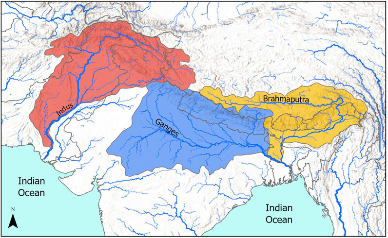
Figure 1. WBM simulation domain that is a subset of the MERIT-Plus river network (Prusevich et al., 2024) for drainage basins of the Indus (red), Ganges (blue), and Brahmaputra (yellow).

The seasonal and long-term changes in aquifer and groundwater storage are major factors in the origin of gravity anomalies detected by the GRACE program satellites (Scanlon et al., 2018; Scanlon et al., 2019). The GRACE mascon, or mass concentration, is a commonly used spatial unit for evaluating the anomalies from GRACE observations; they are tiles over the land and ocean surface of approximately 3° by 3° equivalent areas (Loomis et al., 2021). An aquifer and groundwater process simulation module in WBM [see documentation in (WBM Contributors, 2022)] makes it suitable for assessing changes in TWS and exploring the magnitudes of the contributing factors. The module implementation draws heavily from the USGS MODFLOW model, a widely used software package for aquifer and groundwater simulations (Harbaugh, 2005; Langevin et al., 2017). In this work, the simulations use aquifer properties and geometry from de Graaf et al. (2015) and de Graaf et al. (2017). The WBM groundwater module is fully integrated with other surface and subsurface hydrological processes and anthropogenic water withdrawals, allowing us to dynamically estimate aquifer storage changes. A list of all WBM simulated instantaneous water storage components of TWS is given in Table 1.

Table 1

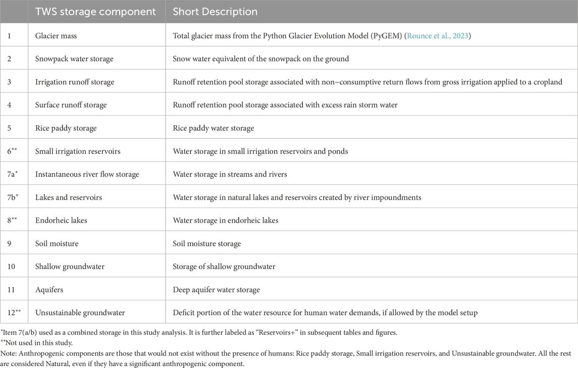
Table 1. Total Water Storage components modeled by the Water Balance Model.

2.2 Model input and parameterization

For this study, we used an extended set of natural and anthropogenic processes in the model setup (Table 2).

Table 2

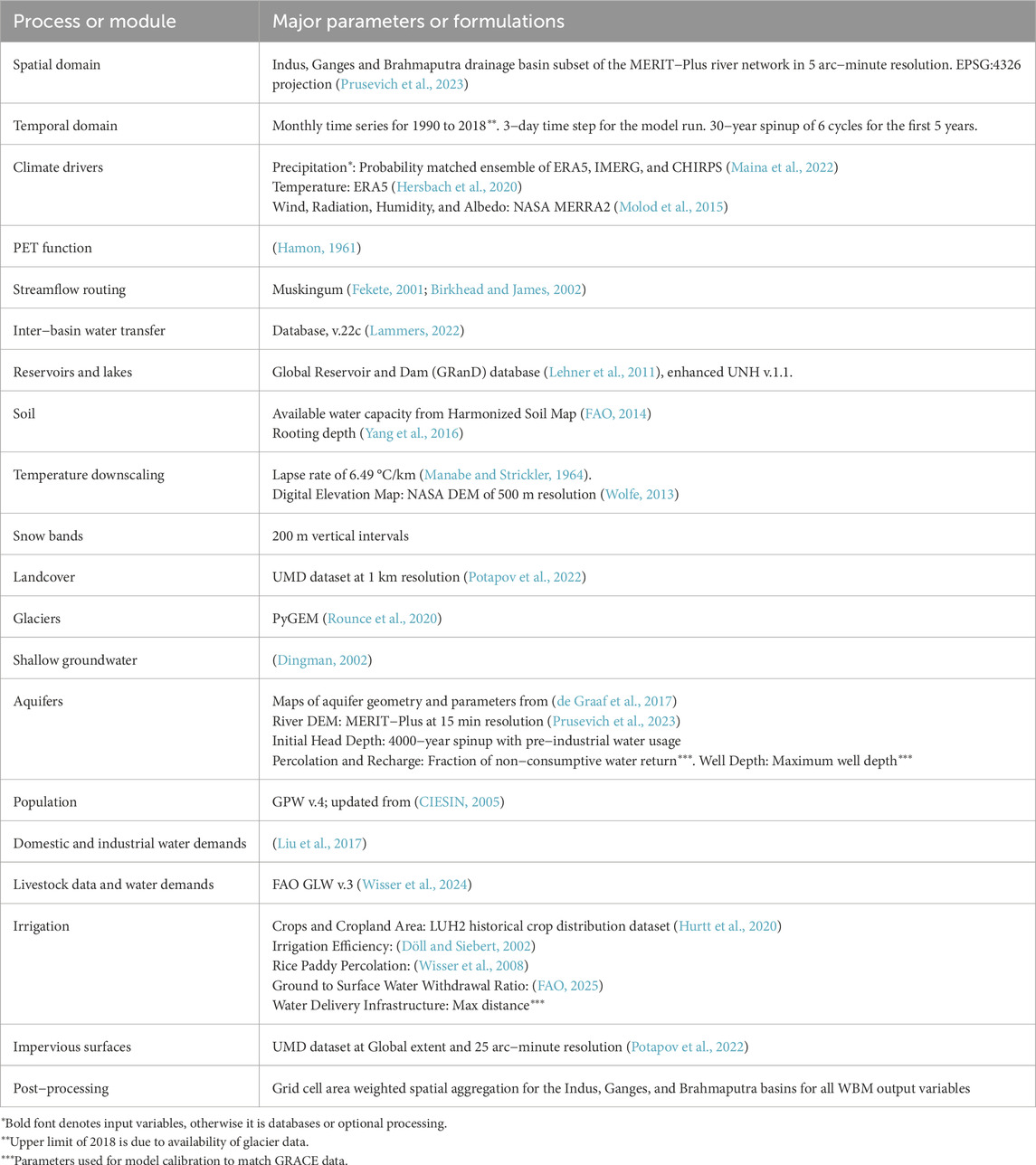
Table 2. WBM model setup configuration and input data.

Natural processes parameters describing evapotranspiration, runoff generation, and river routing were set to the default values established to be least biased for global simulations and exhibit minimal bias in temperate forested and montane watersheds (Fekete et al., 2004; Wisser et al., 2010a; Grogan et al., 2022).

Parameter tuning for anthropogenic processes (irrigation and other human use water withdrawals) was carried out as these processes have wide uncertainty and process variability depending on the local/regional practices, water use technologies, and regulations (Mohan et al., 2024). While most model inputs and parameters for these anthropogenic processes listed in Table 3 are used from the referenced data sources, three parameters require calibration. They are known to have a high level of uncertainty (Wisser et al., 2008; Zuidema et al., 2020) and, thus, can affect long-term TWS trends over this region:

a) The distance at which irrigation water withdrawals can access stream and reservoir storage water (“IrrSearchDist”). This variable represents local and regional development of irrigation water delivery hydro-infrastructure, such as stream/reservoir water diversion locks, canals, levadas, or pipelines.

b) Maximum groundwater well depth limiting access for irrigation water withdrawals from aquifers (“wellMax”). The regional variability of irrigation well depth depends on factors such as the cost of water pumping and extraction, as well as the availability of other water sources (e.g., streams and reservoirs) (Jasechko and Perrone, 2021; Alkon et al., 2024). Here, we vary the well depth limit with the same value over the entire IGB domain.

c) The fraction of non-consumptive irrigation water that recharges groundwater (“ReturnCoeff”). The groundwater portion of the non-consumptive irrigation water percolates to shallow groundwater first and then to deep aquifers. The other portion of the non-consumptive irrigation water goes to the irrigation runoff storage pools that generate irrigation return flow to local streams. The non-consumptive irrigation water is also called inefficient irrigation water and depends on available irrigation technologies and farming practices (Zuidema et al., 2020). In these basins, irrigation efficiency is between 45% and 66% of water applied to the crop fields (Döll and Siebert, 2002). The WBM “ReturnCoeff'' input parameter that controls the ratio between groundwater and surface runoff portion of non-consumptive irrigation water is used as a proxy for the groundwater recharge rate of non-consumptive irrigation water.

Table 3

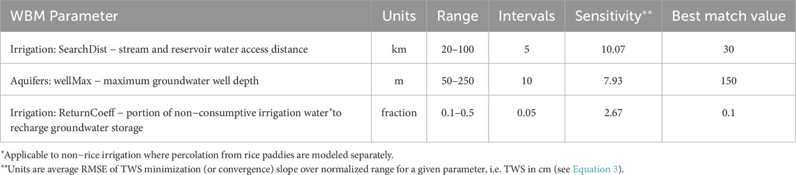
Table 3. Permutation of the WBM input parameters to minimize output deviation from the observed TWS (GRACE satellite mass concentration anomalies).

These parameters were optimized for the best fit to observations using a discrete chi-square error minimization technique with the amoeba (Nelder–Mead simplex) algorithm (Press et al., 1992). We used rounding of the new evaluated parameters to the discrete value nodes by the “Interval” parameter (Harvey, 1982) in Table 3. The function to fit was a monthly observed TWS time series from the GRACE satellite mass concentration anomalies (mascon) (Loomis et al., 2021) aggregated to the river basin area using weighted averages of the 3 × 3 arc degree tiles (Tellus, 2018). The resulting chi-square value (χ²) of the discrete optimized (“Best Match Value” in Table 3) was 13.98. According to the method (Press et al., 1992), its division by the chi-square distribution degree of freedom (ν = 165 in this study) yields the match distribution normalized standard error that, in order to be valid, must be less than one; that is, ${\sigma }^2={\chi }^2/\nu \le 1$. In our case, we have 13.98/165 ≤ 1, which indicates the validity of the minimization. The number of amoeba iterations from the median range values in Table 3 to find the best match was 12. The χ² and ν function minimization metrics are defined by Press et al. (1992):

${\chi }^2={\displaystyle \sum _{i-1}^N}{\left(\frac{y_i-y\left(x_i;a_1...a_M\right)}{{\sigma }_i}\right)}^2(1)$

and

$\mathbf{\nu }=N-M(2)$

where $\mathbf{\nu }$ is the chi-square distribution degree of freedom that is large enough ($\mathbf{\nu }$ = 150 in this study and must be >3) to ensure the validity of the minimization, N = 168 is the number of observation time series points (GRACE monthly data from 2002–04 to 2018–12 with some data gaps), and M = 3 is the number of function parameters to optimize (WBM input parameters) described above. Values for σ_i are all set to a constant of 1 due to unknown values for the GRACE mascons and, therefore, provide no scaling to the data value estimates.

Resultant parameter estimates for the three factors included are presented in Table 3 and were determined uniformly over the IGB domain. Irrigation search distance, which represents how far a grid cell can search for water to meet its demand, overestimates mean canal lengths, which for India are 4.67 ± 10.42 km (IWRIS, 2024). GRACE anomalies were best captured when irrigation water withdrawals were limited when the head fell below 150 m below grade. Over most of the regions where irrigation was limited, median well depths rarely exceed 100 m, so aquifer head below 150 m should be locally limiting to continued abstractions (Sarkar, 2011; Jasechko and Perrone, 2021). Irrigation return coefficients are expected to have a wide range over the domain, with an expected range indicated in Table 3 (Altafi Dadgar et al., 2020). The best match value of 0.1 means that 10% of the irrigation return water goes to the aquifer and 90% goes to surface flow. This is not designed to reproduce field-level irrigation practices but reflects broader-scale mean infiltration and percolation rates. Logically, it is in people’s interest to limit percolation because surface runoff is easier to recapture, and they may have many ways to limit that percolation in the crop land, such as using a clay base layer or adding organic matter to crop fields.

The sensitivity analysis of the WBM parameters used in this model optimization was conducted by evaluating their contribution to minimizing the chi-square function (Equation 1) described above, which fits the model output to observed GRACE gravity anomalies within the study area. This approach allows us to compare the relative influence of each permuted control parameter (listed in Column 1 of Table 4) and identify the most impactful ones. This sensitivity analysis approach uses the Radon–Nikodym equation to find the convergence relationship of contributing parameters within the same measurable space defined in the chi-square formulation (Billingsley, 2012) and normalized by the tested range of the variable ${\Delta }_{Var}$:

$S_{Var}^{TWS}=\frac{{\displaystyle {\int }_A}\sqrt{{\chi }^2}dVar}{{\Delta }_{Var}}(3)$

where $S_{Var}^{TWS}$ is the model sensitivity of TWS output to observed GRACE values on the given input parameter. ${\chi }^2$ is the chi-square function (Equation 1) used to find the best calibration value for that parameter, and A is the permutation space used by the chi-square minimization process.

Table 4

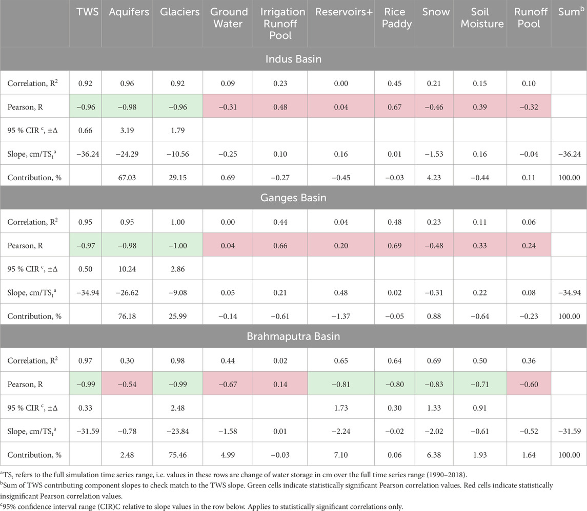
Table 4. Contribution of TWS components to the long term TWS trend.

The calculated sensitivity metric (Table 3) indicates that the irrigation search distance and maximum well depth parameters are sensitive to calculated TWS and impact the model calibration the most. The irrigation return coefficient has a lesser sensitivity but is still important for the calibration, considering its relatively small calibration range of 0.4 fraction units.

In order to demonstrate the relative sensitivity of the calibrated parameters to a few other model inputs, we performed additional runs with alternative climate drivers and some of the hydro-infrastructure turned off. Replacing the precipitation driver for this region (Maina et al., 2022) with MERRA2 precipitation (Molod et al., 2015) decreased TWS vs. GRACE root mean square error (RMSE) relative to the optimized run by 2.31 cm, 1.84 cm, and −0.28 cm in the IGB basins, respectively. Replacing air temperature with MERRA2 data yielded the change by 0.08 cm, 1.1 cm, and −0.03 cm. Removing dams, reservoirs, and inter-basin hydrological transfers resulted in 0.01 cm, 0.02 cm, and 0.00 cm, respectively. These results indicate that model parameterization by the three required parameters (Table 3) has a stronger impact on the TWS vs. GRACE match than either precipitation, temperature, or river dam storage, despite a widely accepted understanding that hydrological models are more sensitive to precipitation than other inputs (Bierkens, 2015).

2.3 Model assumptions and uncertainties

The model configuration (Table 2) is based on the fundamental assumptions that all or most of the hydrological processes affecting individual water storage areas contributing to TWS and listed in Table 1 are strongly affected by the anthropogenic interventions to the water cycle in this geographical area and, specifically, in the basins of the Indus, Ganges, and Brahmaputra containing almost a billion people and one of the highest agricultural land use intensities in the world. Assumptions for the formulation and numerical implementation in the model code for each of the parameters listed in Table 2 are discussed, and details are provided by Grogan et al. (2022).

Uncertainties of the model’s simulated output variables strongly depend on the availability and quality of the input data. The climate driver data used in these simulations, referenced in Table 2, were chosen by NASA’s High Mountain Asia program specifically for the IGB basins (Mishra et al., 2021). Other input datasets were also chosen to represent the best available data on the global and regional scales that are suitable for the WBM simulations.

Aside from TWS, validation of the model results was carried out using a standard WBM validation tool (WBM Contributors, 2022) by matching the simulated to observed streamflow from global GRDC data (GRDC, 2025), which include seven sites within the study domain. The Nash–Sutcliffe coefficient for those ranges between 0.68 and 0.97, which indicates a statistically valid and good match (Supplementary Section S4).

Validating the modeled groundwater and aquifer storage is a challenge. In-situ well data cannot be directly compared to the regional-scale aquifer simulations in WBM, as the latter has large area grid cells while the in situ wells are located based on local topography, geology, and survey data to maximize the water quality and yield. A qualitative comparison of spatial patterns (maps) for the groundwater storage changes by in situ well data (Bhanja et al., 2020) vs. the model output, which indicates a reasonable match (Supplementary Section S5). Basin-wide assessment of observed groundwater level measurements in terms of the metric of groundwater storage anomalies (GWSA_obs) from Bhanja et al. (2020) and compared to those aggregated from WBM simulated aquifers for India portions of the simulation domain (Supplementary Table S1) indicates a reasonable match for the validation of the WBM modeled groundwater and aquifer storage.

The well depth limit of 150 m used in the WBM aquifer modeling (Table 3) may appear unreasonably high. This bias can be estimated relative to actual well depths in the study domain. The hydrological modeling is done over 15 arc-minute spatial resolution grid cells (or approximately 100 km² (10 km × 10 km) cell area) where the well depth threshold is accounted for relative to the average elevation above sea level. In reality, wells are often drilled at the lower/bottom sections of the surrounding landscape and less frequently at the top or middle of the hills. The surface roughness (MSRE of the average elevation) is 93.7 m over irrigated land in the study basins derived from grid cells in 5-minute resolution from a 500 m DEM (NASA, 2021). We suggest that the bias is up to 93.7 m. The difference of 150–93.7 = 56.3 m closely matches the most common well depth in India, which is typically less than 60 m, according to the Ministry of Water Resources of India documents (MoJS, 2024).

3 Methods: time-series analysis of TWS and its components

WBM estimates of TWS exhibit low error against observed TWS anomalies from GRACE but permit the decomposition of the specific pools representing water in the critical zone. There are a number of statistical analysis methods for this kind of time series (TS) data (Bruning and Kintz, 1997; Velicer and Fava, 2003; Ritter and Muñoz-Carpena, 2013; Mudelsee, 2019) that target decomposition of the TS data to the trend and seasonal variability features, including those that were applied to the TWS and GRACE data (e.g., Wu et al. (2021) and Scanlon et al. (2023)). In this study, we chose two TS decomposition methods to apply to our data: (1) classical and (2) singular spectrum analysis (SSA) decomposition (Broomhead and King, 1986; Hassani, 2022). The former is relatively simple and widely used for a wide range of studies in economic, social, and climate studies (Mudelsee, 2019), while SSA decomposition is more complex and provides finer details of the TS trends and seasonal signals than the classical TS decomposition. Below, we present both time series analysis approaches and discuss their results applied to long-term and seasonal contributions to TWS from the individual water storage components (Table 2).

3.1 Analysis by classical time-series decomposition

Classical decomposition calculates trend, seasonal, and residual TS components. The trend or long-cycle TS component ${\widehat{T}}_t$ is defined as a running average by the annual kernel length K, which is 12 to correspond to a year of monthly TS data.

${\widehat{T}}_t={\displaystyle \sum _{k=-K/2}^{K/2}}\left(y_{t+K}\right)/K(4)$

The seasonal component (monthly time steps in this study) of the decomposition is defined as de-trended averages of the time series values within each year y_t, that is, sub-year (monthly) climatologies:

${\widehat{S}}_t={\displaystyle \sum _{n=1}^{n=N}}\left(y_t^n-{\widehat{T}}_t\right)/N(5)$

where t in Equation 5 is an index of time-series seasonal units (e.g., 1–12 for the monthly time series data), n is an index of a yearly cycle, and N is the number of yearly cycles in the data, which essentially is a number of years in the simulated TS. The residuals ${\widehat{R}}_t$ of the classical time series decompositions are defined as

${\widehat{R}}_t=y_t-{\widehat{T}}_t-{\widehat{S}}_t(6)$

We have applied this decomposition method to the TWS time series for all nine contributing TWS variables in each study basin (Supplementary Section S1).

3.1.1 Contribution of TWS components to the TWS long-term trend

The time-series decomposition trend component is used as source data or variables for the long-term trend analysis (Equation 4) applied to variable anomaly values $y_t$:

$y_t=y_t^{original}-{\overline{y}}_t(7)$

where ${\overline{y}}_t$ is the time series average. The resulting trend line ${\widehat{T}}_t$ is then used to calculate the statistical regression slope (time series trend). While the TWS time series are not strictly linear (Figure 2), we still used the regression analysis slopes for the long-term trend evaluation and quantification as a reasonable approximation. The regression slope/trend of a variable $y_t$ is calculated using time as an abscissa axis, where (t,y) points represent a monthly time series:

$Slope=\frac{\sum \left(t-\overline{t}\right)\left(y-\overline{y}\right)}{\sum {\left(t-{\overline{y}}_t\right)}^2}(8)$

Figure 2

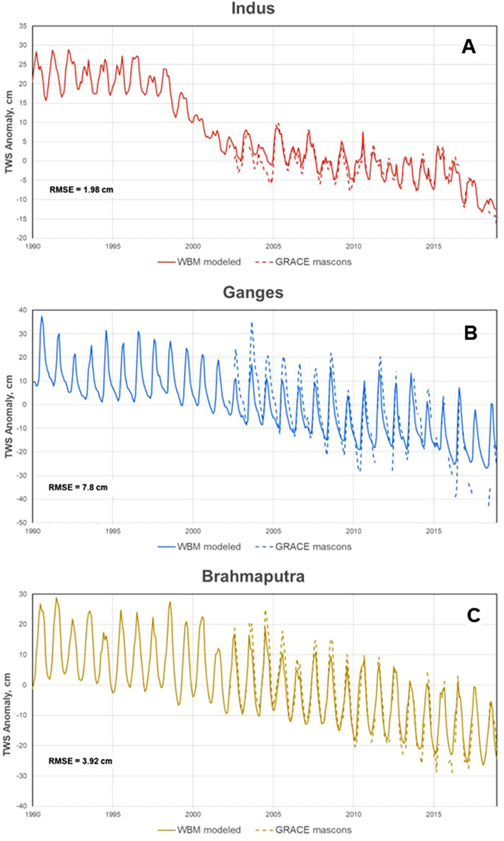
Figure 2. WBM modeled (solid lines) vs. GRACE mascons (dashed lines beginning in year 2002) Total Water Storage (TWS) anomalies for the Indus (panel A, red lines), Ganges (B, blue lines), and Brahmaputra (C, tan lines) basins. Anomalies are calculated relative to mean values of monthly time series for years 2002–2018.

The confidence interval for the regression slope is determined using a basic statistical formulation (Bruning and Kintz, 1997). For example, for a 95% confidence interval, the equation is:

${\widehat{y}}_0\pm t_{crit}^{0.05}·s.e.(9)$

where the standard error of the prediction is

$s.e.=s_{yx}\sqrt{\frac{1}{n}+\frac{{\left(x_0-\overline{x}\right)}^2}{{SS}_x}}(10)$

where s_yx is the standard error of the predicted y-values in the regression standard deviation, SS_x is the sum of squares of deviations of data points from their mean, and $t_{crit}^{0.05}$ is the t-value of Student’s t-distribution for the cutoff probability value of 0.05 (i.e., 95 %).

Calculation of a given water storage term contribution to TWS is done by the ratio of their individual trend slopes. Because TWS is a sum of contributing storage terms/variables, our assumption is that the trend and regression slope of TWS is the simple additive product of its contributive components. It is also based on a reasonable approximation of tangent additivity for shallow slopes/angles where the function’s second derivative is near zero. Therefore, the ratio of a component trend slope Sc_i to the TWS trend slope S_TWS is the metric of the TWS change contribution Cc_i from the given component i:

${Cc}_i=\frac{{Sc}_i}{S_{TWS}}100\%(11)$

where slopes Sc_i and S_TWS are found by the statistical regression of variable values against time.

3.1.2 Contribution of TWS components to seasonal TS variability

The metric for the contribution of water storage components to the TWS seasonal variability is a ratio of the amplitude of the contributing component signal to that of TWS, with a timing-shift correction. The timing-shift correction is required because, unlike the trend, the seasonal signal has a fixed periodic 12-month cycle, which, in turn, may not match the seasonal TWS (minimum and maximum) cycle timing. So, the timing shift is defined as a difference between the contributing components and the TWS cycle timing. For example, the maximum of the seasonal TWS signal in the Ganges basin is September, but it is April for the glacier storage, making the timing shift for the latter to have a value of 5 months. In addition, the periodic seasonal signal of TWS and all its components is approximately sinusoidal in shape. The formulation of the numerical value of the seasonal signal contribution of a given TWS component (e.g., glaciers) to the TWS seasonal signal is provided below as a two-step procedure. First, the seasonal signal of TS decomposition (Supplementary Figure S4) is approximated to a sinusoidal function $S_t^f$ with two control parameters for the amplitude $A_s$ and timing shift $M_s$ in the form of:

$S_t^f=A_s\mathit{Sin}\left(\frac{2\pi }{12}\left(t_m+M_s\right)\right)(12)$

where $t_m$ is a discrete monthly abscissa variable, and $\frac{2\pi }{12}$ is a fixed periodicity scaling factor accounting for the 12-month seasonal cycle. The values of the amplitude and timing-shift parameters $\left(A_s,M_s\right)$ are found by fitting to the original seasonal signal values ${\widehat{S}}_t$ (Equation 5) by chi-square error minimization, assuming undefined statistics for the function parameter values:

${\chi }^2={\displaystyle \sum _{i=1}^{12}}{\left({\widehat{S}}_t-S_t^f\left(A_s,M_s\right)\right)}^2(13)$

The values of $A_s$ and $M_s$ and graphs of the fit are shown in Table 5 and Supplementary Figure S4. The error function (Equation 13) minimization is evaluated by the MS Excel equation solver tool using the generalized reduced gradient nonlinear method (El-Kady et al., 1987) applied to the data in this work spreadsheet, available as part of the Supplementary Material.

Table 5

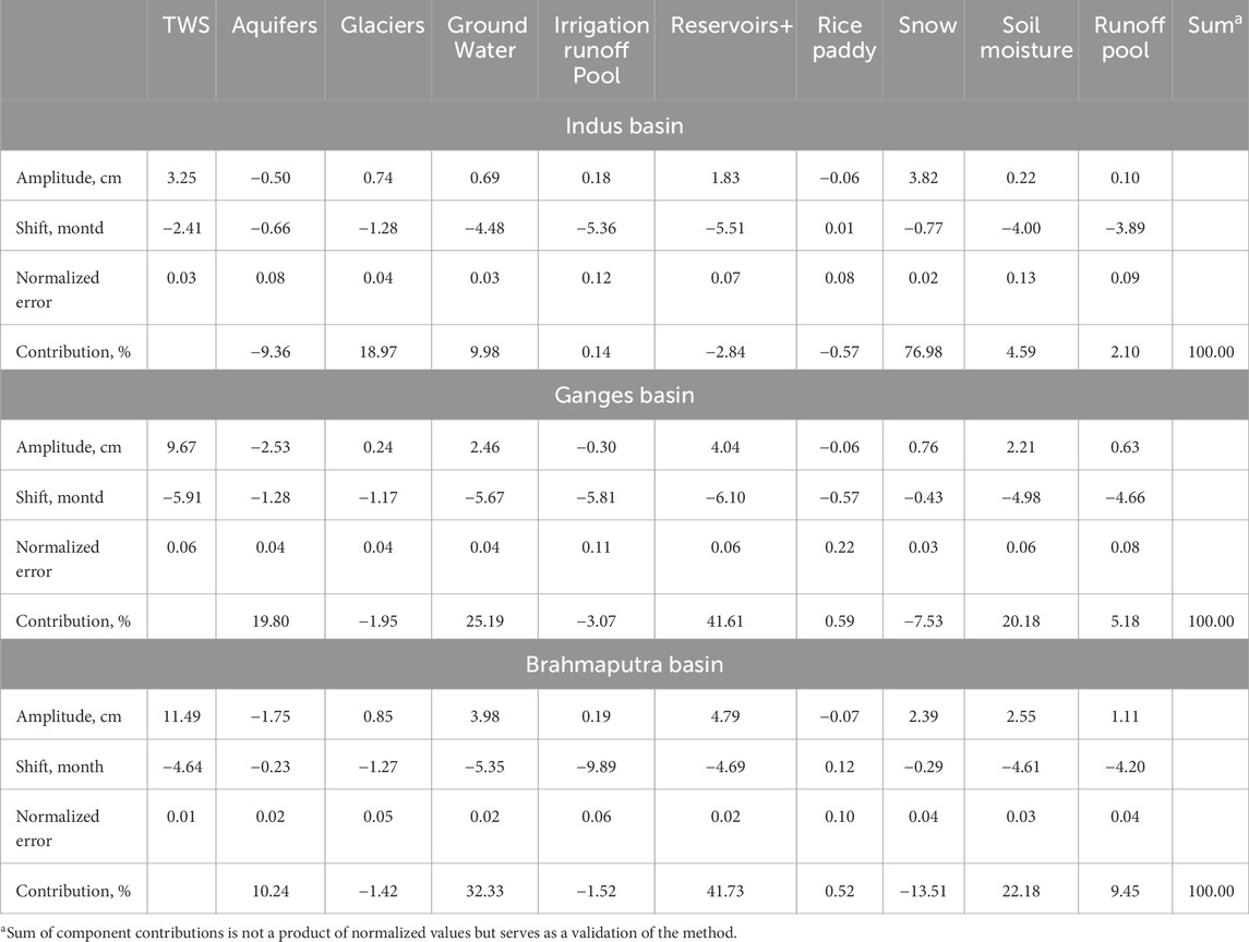
Table 5. Contribution of TWS components to the seasonal TWS variability.

Second, the sinusoidal function parameters $\left(A_s,M_s\right)$ are used to calculate the contribution of each water storage component i to TWS as a ratio of sinusoid amplitude $A_s^i$ corrected to the timing shift between extremes of the component ($\left.M_s^i\right)$ and TWS ($M_s^{TWS}$) as follows:

${Cc}_i^S=\frac{A_s^i}{A_s^{TWS}}\mathit{Cos}\left(\frac{2\pi }{12}\left(M_s^i+M_s^{TWS}\right)\right)100\%(14)$

where superscript S refers to the seasonal contribution of the component i to distinguish it from the one in Equation 10 for the long-term trend contribution.

3.2 Analysis by the singular spectrum time series decomposition

To test the sensitivity of our findings to the choice of decomposition method, we applied singular spectrum analysis (SSA) for time series decomposition of the TWS data and its components. This technique is more advanced than the classical time series decomposition used in the previous section, as it can capture the nonlinear behavior of long-term trends and seasonal variability. This alternative method can assess whether the classical analysis misses any important features relevant to the nonlinearity. We found that SSA decomposition and component analysis yielded similar results to the classical approach and chose the classical approach in the interest of reproducibility and ease of interpretation. The SSA data are provided in the (Supplementary Section S2; Supplementary Figures S5–S9), and below we briefly summarize the SSA formulations and parameterization used in this study.

In addition to the classical time series decomposition, SSA was developed to address all long-term, nonlinear seasonal, and residual noise signal behavior along the time dimension (Golyandina and Zhigliavskii, 2013). SSA decomposition finds temporal principal components of the signal where their time-value paired modes relate to the first order (long-term trend), second order (seasonal variability), third order (sub-seasonal variability), and phase quadrature while minimizing the residual noise. Intrinsically, the time series is transformed into a trajectory matrix using embedding, and singular value decomposition is applied to extract eigenvalues and eigenvectors. The signal window width of the SSA determines the longest periodicity for the first-order mode, and this parameter, along with a few others, is a required input to the SSA routines, along with the time series data itself. A detailed formulation of the SSA procedure specifically used in this study can be found in Tiwari and Rekapalli (2020).

SSA functions are available in many popular scripting languages, including MATLAB and R (Golyandina et al., 2018; Tiwari and Rekapalli, 2020). In this study, SSA was computed with the MATLAB function trenddecomp on each of the 348-month (29 years) WBM time series starting in January 1990. The lag parameter for the SSA analysis was set to 36 months, and the number of desired seasons was set to 6. A lag setting of 36, a multiple of the annual cycle (12 months), was found by trial and error with alternative settings (e.g., 24 months and 48 months) to adequately resolve the annual cycle from longer (trend) and shorter periods. A setting of 6 for the number of desired seasons allowed for the possibility that the annual cycle might not be the most important mode of seasonal variability. The SSA seasonal mode finally selected to represent the annual cycle is the mode most highly correlated with a time series of the long-term monthly means of the WBM variable repeated each year. For 28 of the 30 runs (10 WBM variables² × 3 basins), the final seasonal series was the most important (highest eigenvalue) in the seasonal matrix returned by trenddecomp. For the other two runs, the final seasonal series was the second-most important (Supplementary Figures S5–S7). The component contribution graphs are presented in Supplementary Figures S8, S9, indicating similar results to those using the classical time series decomposition.

4 Results

Results are presented in two groups. The first group describes the output data from the hydrological modeling, primarily focused on total water storage (TWS) and its match to observed GRACE gravity anomalies. The second group provides the results of the statistical analysis of the model output time-series data and quantification of each major hydrological storage component to the TWS changes, providing a quantitative metric of their contributions.

4.1 Hydrological modeling of the total water storage in the study basins

TWS simulated and observed time series data for all three study basins (Figure 2) indicate two major features: (a) long-term TWS decline trends and (b) seasonal variability. The WBM simulation yielded a TWS time series for all three study basins, with the observed TWS data represented by GRACE gravimetric data. Graphs of individual components of TWS are given in the Supplementary Material. The dynamics of TWS change in the Indus basin contrast with those of the Ganges and Brahmaputra. The Indus exhibits less regularity in its seasonal cyclicity and underwent rapid declines from 1998 to 2005 and again after 2015. Early declines from the late 1990s to early 2000s predated the availability of GRACE data but are consistent with aquifer storage trends indicated through gauging data during the time period (MacDonald et al., 2016). The Ganges shows a slow decline beginning in the late 1990s, and the Brahmaputra’s TWS decline began in the early 2000s. For both the Ganges and Brahmaputra, WBM TWS underestimates the increased seasonal variability and storage decline after about 2010. WBM’s estimated TWS anomaly over the Indus basin exhibited a root mean square error (RMSE) less than 2 mm, which is less than 1% of the range of TWS variability (Figure 2a). WBM’s RMSE over the Ganges basin was larger (7.8 mm), dominated by uncharacterized deviations in 2004 and after 2015, but was still approximately 1% of the range in TWS variation (Figure 2b). The 3.9 mm RMSE over the Brahmaputra basin represents approximately 0.7% of the range of TWS variation (Figure 2c). Generally, in both the Ganges and Brahmaputra, it appears that WBM underpredicts the seasonal amplitude of observed TWS. However, both the seasonal cycle and the long-term (decadal) trends match well enough for the use of WBM results for decomposition.

GRACE 3° × 3° mascon tiles (Figure 3a) are shown with the major TWS relevant output variables from the WBM simulation over the IGB domain presented in Figures 3b–f. There is a spatial correspondence between the mascons and the WBM simulated total TWS (Figures 3a,b); however, the resolution mismatch makes it difficult to compare and requires spatial aggregation of high-resolution TWS modeled data to corresponding coarse mascon tile polygons. This aggregation and comparison to the mascon data yields an RSME of 5.12 cm/(17 years), where “17 years” refers to the full range of years between 2002 and 2018. There is also a clear correspondence of TWS to aquifer and glacier storage (Figures 3b,c), which qualitatively indicates that the latter two are the major contributors of TWS change over the time period. The quantitative assessment for the study basins is provided in the next section. Patterns of glacier and snow storage changes match one another but differ in their amplitudes (Figures 3d,e). Irrigated regions limited by aquifer water accessibility due to head depth (Figure 3f) are concentrated in the Indus basin, with fewer areas in the Ganges, and almost none in the Brahmaputra basin.

Figure 3

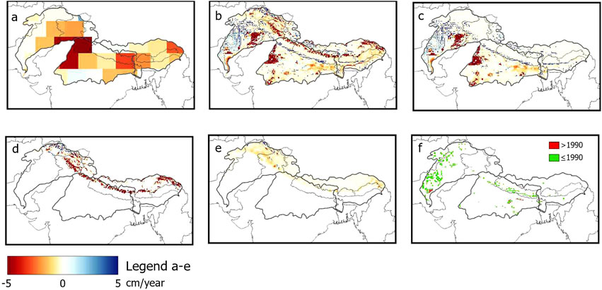
Figure 3. Water storage changed between 1990 and 2018 in the Indus, Ganges and Brahmaputra basins (their boundaries are shown in thick grey lines): (a) GRACE 3x3 arc degree mascon tiles (Tellus, 2018); WBM-simulated: (b) TWS; (c) aquifer; (d) glaciers; (e) snow. (f) Areas with well depth limitations in green color and red color for areas added since 1990.

4.2 Contribution of individual hydrological storage areas to the long-term and seasonal variability of the total water storage

Results of hydrological component contributions to TWS long-term trends and seasonal variability are provided in two sub-sections below.

4.2.1 Contribution of TWS components to the TWS long-term trend

The results of this analysis are given in Table 4 and Figure 4 and indicate that there are only two major contributors to the TWS long-term trends: aquifer and glacier water storage in all three study basins, with a clear difference in actual contribution values. It is also worth noting that the sum value of contributions in Table 4 provides a check on the validity of the assumption of component contribution additivity. A close match to the TWS slope value and 100% of the component contribution sum shows this assumption to be appropriate.

Figure 4

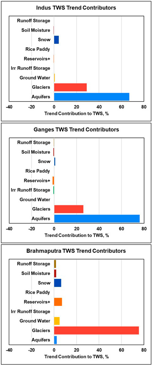
Figure 4. Contribution of individual water storage components to the total water storage (TWS) trends for the three study basins.

The analysis found that the major water storage components contributing to the long-term TWS trend are similar in the Indus and Ganges basins but quite different in the Brahmaputra basin. Aquifer water depletion and receding of glaciers contributes about 67%–76% and 29%–26%, respectively, of TWS decline in the Indus and Ganges basins, while the other storage terms (except for 4.2% contribution of snow in Indus basin) do not affect TWS trends meaningfully (Figure 4). The Brahmaputra basin exhibits TWS decline predominantly due to the melting and loss of glacier mass in the mountains, with smaller contributions of approximately 5%–7% each from snow, reservoir, and groundwater storage terms (Figure 4). The physical and climatological causes of the TWS component temporal dynamics are discussed in the next section to explain the trend contributions and some non-uniformity of TWS decline, especially in the Indus basin (Figure 2a).

4.2.2 Contribution of TWS components to the seasonal TS variability

Water storage component contributions to TWS seasonal variability calculated by Equation 14 are shown in Table 5 and Figure 5. The checksum for component contributions in Table 5 is provided for the purpose of the calculation method validation. Sinusoidal functions were used to calculate a normalized error with respect to measured values for the seasonal signals of the classical TS decomposition for TWS and its component storage areas in the IGB basins (Supplementary Figure S4). This normalized error is given in Table 5, which is an average distance between the original and fit curves (Supplementary Figure S4) relative to the fit curve amplitude. It is a metric of how close the seasonal component is approximated by the sinusoidal function. For example, the irrigation runoff storage pool and rice paddy water have the highest deviation from the sinusoidal curve, which is understandable due to multiple seasonal crop rotations in this part of the world where irrigated rice is harvested up to four times per year, as modeled by WBM (Portmann et al., 2010).

Figure 5

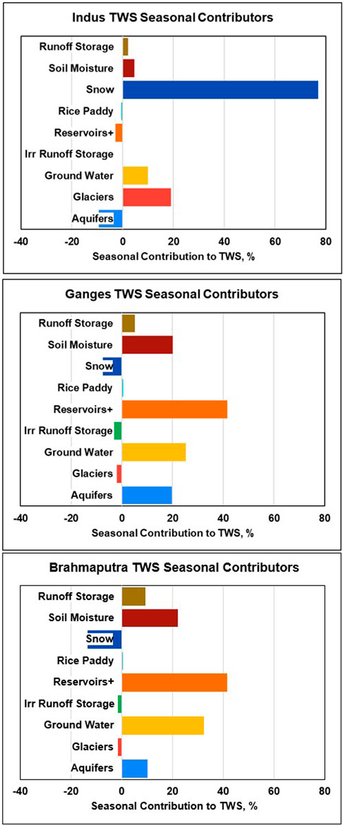
Figure 5. Contribution of specific water storage components to the total water storage seasonal variability for the three study basins.

Unlike the case for the trend contributors (Figure 4) where the Indus and Ganges basins have glaciers and aquifers as the dominant trend contributors with similar magnitudes, the seasonal contributing variables (Figure 5) are quite different and unique only for the Indus showing a single dominant variable (snow) with glaciers, groundwater, and aquifers being important, but less significant. This indicates water storage in high mountain cold regions is an important component in the Indus TWS seasonal variability. The Ganges and Brahmaputra had a greater variety of variables playing important roles in the seasonal contributors, and they had very similar magnitudes across their contributory variables: soil, runoff, and reservoir storage at the land surface, and groundwater with aquifers below. Considering that seasonal TWS and its components peak in the late summer months, these results suggest that monsoon-related hydrological processes are the drivers of the seasonal TWS variability in the Ganges and Brahmaputra basins.

5 Discussion: hydrological interpretation of TWS trends and seasonal variability

Deterministic model simulations recreated trends in TWS in the years 2002–2018 for the IGB basins with 2.0 cm, 7.8 cm, and 3.9 cm RMSE error, respectively. The model recreated 1.1–1.3 cm/y declines in TWS, with local declines in TWS as high as approximately 35 cm/y. The largest contributors to the observed declines in TWS were groundwater in the Indus and Ganges and glacial mass loss in the Brahmaputra. These findings are consistent with recent findings from Maina et al. (2024), using the land surface model NOAH-MP in a data assimilation approach that forced TWS to GRACE observations. Importantly, Maina et al. (2024) identify reductions in streamflow between 2002 and 2017, which we also observe in our simulations (Figure 6). The ability to recreate such findings with a deterministic model provides support for the projection of future changes in TWS, groundwater availability, and irrigation potential for the region.

Figure 6

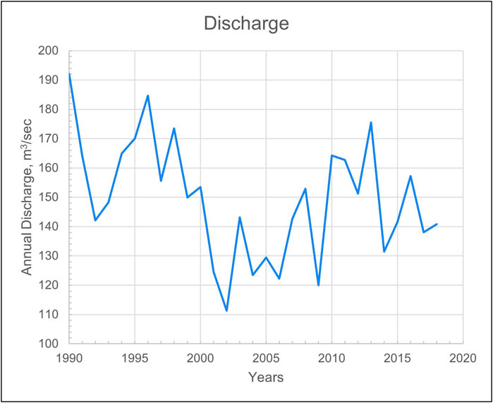
Figure 6. Total river discharge from all three IGB basins over the simulation period.

Total water storage simulated by WBM is composed of nine specific water storage terms listed in Table 1, but their contribution to the TWS trends and seasonal variability is different in each of the three study basins (Figures 4, 5). There are two classes of hydrological processes in WBM: (1) natural and (2) anthropogenic controls on the overland water cycle (Grogan et al., 2022). These two classes were used as a basis for analysis and interpretations. Referencing the WBM modeled processes as natural or anthropogenic does not account for indirectly induced anthropogenic factors, such as climate change, in the climate drivers used in the numerical simulations.

Irrigation is the primary anthropogenic influence on water fluxes contributing to TWS depletion (Grogan et al., 2017). Changes in total irrigated land over the simulation period were different for each of the basins (Figure 7). The Ganges had the steepest increase in the 1990s and into the 2000s, followed by shallower increases later. This had a direct effect on irrigated water use in the basin (Figure 8). The Indus basin experienced a constant rate of increase of irrigated land throughout the study period; however, the extraction of water for irrigation peaks in the early 2000s and is followed by a slow decline. The model captures the observed decrease in aquifer water use in the Indus basin despite the increase in irrigated area because the aquifer head reaches the limiting well depth threshold of 150 m in many regions (Figure 3f). This is confirmed when looking at the model’s total irrigated land area without access to aquifer water due to well depth limitations (Figure 9). These are located mostly in the Indus and less so in the Ganges basins but not in the Brahmaputra (Figure 3f). In the Indus basin, this limitation started after 1998 with a sharp increase to approximately 2000 km² around 2010, localized to areas within the Punjab regions of central Pakistan and western India (Figure 3f). Wells in the region are often 100 m deep (Sarkar, 2011; Jasechko and Perrone, 2021), and prior studies have confirmed problematic localized drawdown in similar regions as predicted here (Arshad et al., 2024). A similar aquifer water access problem started in the Ganges basin beginning in 2005, and its exclusion area was still increasing in 2018. The Brahmaputra shows reduced irrigated lands beginning early in the 2000s; however, water from aquifers remains stable throughout the study period, with increases in aquifer water limits beginning around 2005. This suggests that less water is available from non-aquifer sources or more water is applied per unit area in irrigated cropland, primarily due to increased air temperature and potential evapotranspiration during the crop planting seasons.

Figure 7

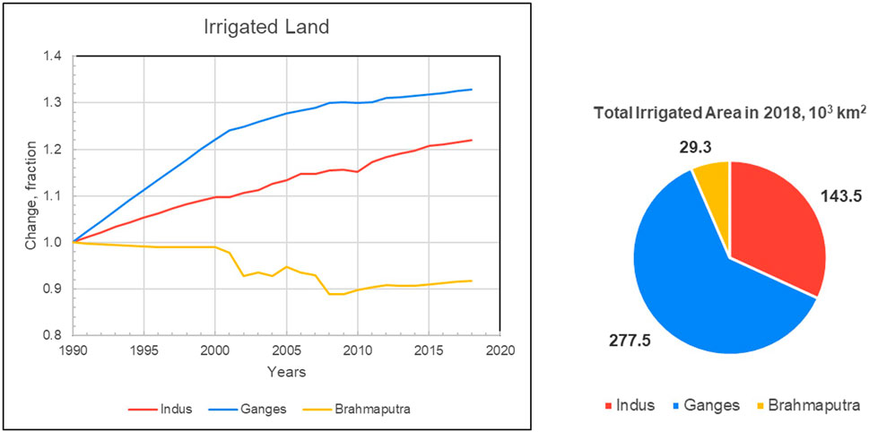
Figure 7. Indus, Ganges and Brahmaputra irrigated land and its change over the WBM simulation period (left panel) along with the pie chart of total irrigated land in each basin (right panel). Data source: (Hurtt et al., 2020).

Figure 8

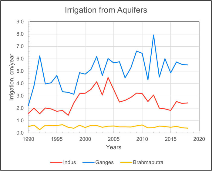
Figure 8. Irrigation water use from aquifers in the study basins. Units are water depth equivalent (in centimeters) of the whole area of a basin. Note: mean annual irrigation water applied to the fields, of which irrigation water from aquifers is only a portion, would be higher. Units are chosen to match GRACE mascons (Tellus, 2018).

Figure 9

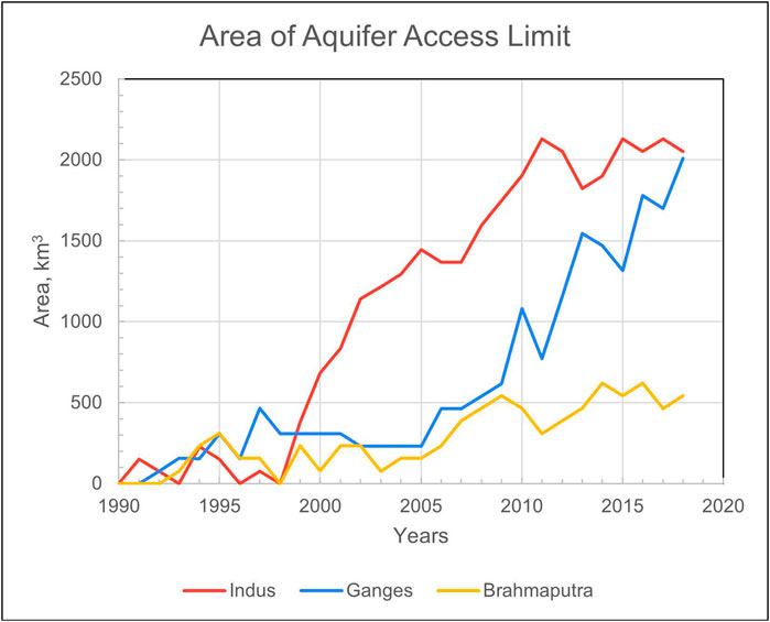
Figure 9. Total irrigated land area without access to aquifer water due to well depth limitations in the study basins. The well depth limit of 150 m was found by the model parameter optimization based on the match of the model output to GRACE mascon data (see Table 3).

The variables contributing to long-term TWS trends (Figure 4) indicate that approximately 70% of the trend is due to depletion of aquifers in the Indus and Ganges, and only a small percentage in the Brahmaputra. Moreover, the nonlinear changes of TWS in the Indus basin (Figure 2a) result from a stable aquifer with sufficient water resource availability for irrigation until about the year 1998. After that, increasing cropland area and irrigation water demand (Figure 7) caused aquifer water use to increase (Figure 8). This triggered a decline in aquifer storage and a drop in TWS from 1998 to 2005. During this time, the aquifer head fell below maximum well depth limits with increasing frequency (Figure 9), leading to a slower decline of TWS in the Indus basin as extraction became impractical or too expensive (Turner et al., 2019). The accelerated drop in the Indus basin during the last 3 years of the simulation (2015–2018; Figure 2a) is due to a decline of snowpack and reservoir storage along with a steeper decline of glacier volume due to step-like increase of the air temperatures by approximately 1°C at higher elevations (>2000 m) during corresponding years of 2015–2018 (Supplementary Figure S10).

Natural factors (not directly anthropogenic) in the long-term TWS trends were found to be primarily contributed by changes in glacier volume/mass in all three study basins (Figure 3). Glacial mass loss is driven by atmospheric warming (Rounce et al., 2023) and, in a few regions, including the Karakorum, in the upstream catchments of the Indus River, the drying potential of warming is partly offset by increased precipitation (Farinotti et al., 2020). Glacier mass balance estimates from the Python Glacier Evolution Model (PyGEM (Rounce et al., 2023)) are an input to WBM. These glacier mass balance estimates were calibrated against glacier-wide mass balance data (Hugonnet et al., 2021) and validated against in situ measurements (WGMS, 2025). Thus, specific drivers and mechanisms of glacier mass loss are not discussed here, but we can summarize the glacier mass loss dynamics in the study basins based on the glacier data driving the simulations (Rounce et al., 2020).

Total glacier mass in the Indus basin is about five times that in the other two basins (Figure 10b), but its slower rate of mass loss (Figure 10a) makes the basin-wide TWS contribution about the same as in the Ganges (Figure 10c). Glaciers in those two basins account for approximately 30% of TWS loss (Figure 4), which is approximately 10 cm over the 29-year simulation time period (Figure 10c). In the Brahmaputra, glacier mass change is the only major factor of TWS decline, comprising approximately 25 cm of water loss (Figure 10c). The glacier decline lines are quasi-linear in the Indus and Ganges, with increasing negative decline in the Brahmaputra catchment relative to the Indus and Ganges (Figures 10a,c).

Figure 10

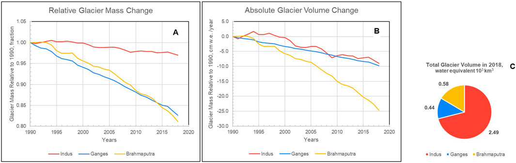
Figure 10. Glacier volume/mass and their changes over the simulation time period in the Indus (red), Ganges (blue) and Brahmaputra (orange); (a) relative glacier volume change as a ratio to the 1990 volume, (b) total glacier volume, and (c) absolute glacier volume change as a difference relative to 1990. Centimeter (cm) units on graph (c) are equivalent water layer thickness over basin area of the glacier volume.

While long-term TWS change contributors are similar in the Indus and Ganges and different in the Brahmaputra, the seasonal variability contributors are different in the Indus and similar in the Ganges and Brahmaputra (compare Figures 4 and 5). The seasonality of TWS in the Indus is driven by snow and some glacier melt and is negatively offset by aquifer storage depletion in the dry season (winter) (Figure 5). In the Ganges and Brahmaputra, most variables contribute to the seasonal trend with negative offsets by snow and glaciers (Figure 5). The seasonality of TWS in the Indus basin is driven by the high mountain cold regions in the basin. In the other two basins, the primary driver of TWS seasonality change is water storage in the lowland plains through components such as reservoirs, shallow groundwater, and soils.

The maximum seasonal TWS signal for the Indus is in April, when snow and glacier mass is the highest (Supplementary Figure S4), but the peak TWS signal is at the end of the monsoon in August for both the Ganges and Brahmaputra. The amplitude of the seasonal variability is approximately 4–5 times higher in the monsoon-affected Ganges and Brahmaputra basins than in the Indus, and this overwhelms high-mountain storage (Supplementary Figure S4). There is a smaller TWS signal in July and August in the Indus due to monsoon precipitation (Supplementary Figure S4 left column). That finding corresponds well to the average monsoon season (June–August) precipitation in the IGB basins as 91 mm/month, 274 mm/month, and 365 mm/month, respectively, affect not only the timing but also the amplitude of seasonal variability in the lowland water storage (Supplementary Figure S4).

The reduced seasonal amplitude of modeled TWS relative to the GRACE observations for the Ganges and Brahmaputra (Figures 2b,c) is affected by storage components that have high seasonal variability and a significant contribution to the seasonal signal of TWS (Table 5; Figure 5). These are surface and near-surface water pools, such as soil moisture, reservoirs, lakes, and rivers (labeled as Reservoir+ on the tables and figures), in which seasonal variability is likely underestimated by the model. The underestimation may come from not including the small irrigation reservoirs (Wisser et al., 2010b) which are full during the monsoon season (maximum of seasonal TWS) and empty by the end of the dry season (minimum of seasonal TWS) and, thus, causing underestimation of modeled seasonal variability for the Ganges and Brahmaputra while not impacting that for Indus (Figure 2a). The Reservoir+ factor is small for the Indus basin (Table 5; Figure 5). We did not include small irrigation reservoirs in this study as these are not observations but speculatively derived from modeling (Wisser et al., 2010b).

A brief comment can be made regarding the future projections for water storage in the IGB basins. The authors conducted WBM simulations over a global spatial domain with a coarse resolution of 15 arc minutes, utilizing climate, agricultural, and socio-economic datasets from the CMIP6 repositories to assess the impacts of TWS changes on sea level rise. They found that water storage dynamics are expected to remain relatively stable over the next few decades, as aquifer depletion and mountain glacier melting continue. However, by the mid- and late century, glacier mass loss will slow as most small glaciers will have melted (Rounce et al., 2025). Meanwhile, aquifer depletion is anticipated to stabilize eventually. This stabilization is primarily due to limitations in water accessibility resulting from well depth constraints, which are in turn influenced by economic factors such as the cost of water extraction and return on investment.

6 Conclusion

The findings and interpretation of TWS component contributions to long-term trends and seasonal variability in the three study basins are summarized in Table 6. The Indus and Ganges basins appear to have higher water resource stress, causing TWS to decline due to aquifer overdraft. The Brahmaputra basin has a much smaller irrigated land area with sufficient water resources, but glaciers within the basin have lost mass at a higher rate, making glacier recession the dominant driver for the TWS decline. Hydrological storage components of long-term trends are similar in the Indus and Ganges, but for the seasonal variability, the Ganges and Brahmaputra are similar. The spatial location of these three drainage basins from northwest to southeast, following along the Hindu Kush, Karakorum, and Himalayan mountain ranges, and the Indus and Brahmaputra appear to be end-members of a spectrum of TWS control factors (i.e., aquifers vs. glaciers), with the Ganges appearing as a middle member sharing each of the end-member patterns.

Table 6

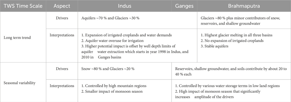
Table 6. Summary of TWS component contributions in the Indus, Ganges, and Brahmaputra basins.

We have introduced a method for determining land surface total water storage using a global hydrological model that deterministically captures natural hydro-climatological variability and highlights multiple variables of human water transport, use, and consumption. The decomposition of the TWS trend into its multiple contributing factors can be used to understand the natural and human processes underlying the aggregate measures of TWS and its observation via the GRACE satellite time series and to concisely summarize the complexity of a region’s water balance changes over time. Understanding the spatially heterogeneous drivers of observed TWS decline allows us to translate satellite observations into policy-relevant information. For example, our finding that the primary driver of TWS decline in the Indus basin is groundwater extraction for irrigation supports previous studies calling for an adaptive irrigation policy in that basin to address food and water sustainability goals (Vinca et al., 2021; Smolenaars et al., 2023; Smolenaars et al., 2024). A very different policy recommendation arises from understanding the drivers of TWS decline in the Brahmaputra. In this basin, we find that glacier mass loss is the primary reason for TWS decline, lending support to calls for continued and improved glacier monitoring in the Brahmaputra to better understand climate change impacts on downstream water resources (Azam, 2021). While we would not say that glacier monitoring is unimportant in the Indus basin or that adaptive irrigation policy is unimportant in the Brahmaputra, these results allow for prioritization and understanding of leading versus secondary causes of terrestrial water storage changes.

Because this functionality is built within a process-based global hydrological model, future projections can be used to illuminate those aspects of the hydrological cycle that require additional attention by decision makers to ensure adequate water resources are available for all.

Data availability statement

The original contributions presented in the study are included in the article/Supplementary Material; further inquiries can be directed to the corresponding author.

Author contributions

AP: Conceptualization, data curation, formal analysis, funding acquisition, investigation, methodology, project administration, resources, software, supervision, validation, visualization, writing – original draft, writing – review and editing. RL: Conceptualization, funding acquisition, investigation, methodology, project administration, resources, supervision, writing – review and editing. DG: Writing – review and editing. SZ: Writing – review and editing. DM: Conceptualization, investigation, methodology, writing – review and editing. DR: Data curation, methodology, conceptualization, investigation, resources, writing – review and editing. RH: Methodology, conceptualization, investigation, writing – review and editing. IV: Writing – review and editing.

Funding

The author(s) declare that financial support was received for the research and/or publication of this article. This material was based upon work supported by the National Aeronautical and Space Administration, Earth Science Division’s High Mountain Asia program (grant no. 80NSSC20K1595), Sea Level Change program (grant nos. 80NSSC20K1296 and 80NSSC25K7225), and the Modeling, Analysis, and Prediction program (grant no. 80NSSC24K1576); the National Academies of Science, Engineering and Medicine (grant no. SCON-10000570); and the National Science Foundation program on Innovations at the Nexus of Food, Energy, and Water (grant no. 1855937).

Acknowledgments

We would like to thank Stanley Glidden (UNH) for the Water Balance Model and GIS data support and for creating the map illustrations. We would like to thank numerous reviewers, especially reviewer number 5, for valuable and detailed comments that greatly improved this article.

Conflict of interest

The authors declare that the research was conducted in the absence of any commercial or financial relationships that could be construed as a potential conflict of interest.

Generative AI statement

The author(s) declare that no Generative AI was used in the creation of this manuscript.

Publisher’s note

All claims expressed in this article are solely those of the authors and do not necessarily represent those of their affiliated organizations, or those of the publisher, the editors and the reviewers. Any product that may be evaluated in this article, or claim that may be made by its manufacturer, is not guaranteed or endorsed by the publisher.

Supplementary material

The Supplementary Material for this article can be found online at: https://www.frontiersin.org/articles/10.3389/feart.2025.1551218/full#supplementary-material

Footnotes

¹In this article, we use the term GRACE to describe the combined data from both the GRACE and GRACE-FO missions.

²TWS plus nine individual TWS components (storage areas).

References

Alkon, M., Wang, Y., Harrington, M. R., Shi, C., Kennedy, R., Urpelainen, J., et al. (2024). High resolution prediction and explanation of groundwater depletion across India. Environ. Res. Lett. 19 (4), 044072. doi:10.1088/1748-9326/ad34e5

CrossRef Full Text | Google Scholar

Altafi Dadgar, M., Nakhaei, M., Porhemmat, J., Eliasi, B., and Biswas, A. (2020). Potential groundwater recharge from deep drainage of irrigation water. Sci. Total Environ. 716, 137105. doi:10.1016/j.scitotenv.2020.137105

PubMed Abstract | CrossRef Full Text | Google Scholar

Arshad, A., Mirchi, A., Vilcaez, J., Umar Akbar, M., and Madani, K. (2024). Reconstructing high-resolution groundwater level data using a hybrid random forest model to quantify distributed groundwater changes in the Indus Basin. J. Hydrology 628, 130535. doi:10.1016/j.jhydrol.2023.130535

CrossRef Full Text | Google Scholar

Azam, M. F. (2021). Need of integrated monitoring on reference glacier catchments for future water security in Himalaya. Water Secur. 14, 100098. doi:10.1016/j.wasec.2021.100098

CrossRef Full Text | Google Scholar

Badiani, R., Jessoe, K. K., and Plant, S. (2012). Development and the environment: the implications of agricultural electricity subsidies in India. J. Environ. and Dev. 21 (2), 244–262. doi:10.1177/1070496512442507

CrossRef Full Text | Google Scholar

Bhanja, S. N., Mukherjee, A., and Rodell, M. (2020). Groundwater storage change detection from in situ and GRACE-based estimates in major river basins across India. Hydrological Sci. J. 65 (4), 650–659. doi:10.1080/02626667.2020.1716238

PubMed Abstract | CrossRef Full Text | Google Scholar

Bierkens, M. F. P., and Wada, Y. (2019). Non-renewable groundwater use and groundwater depletion: a review. Environ. Res. Lett. 14 (6), ARTN 063002. doi:10.1088/1748-9326/ab1a5f

CrossRef Full Text | Google Scholar

Bierkens, M. F. P. (2015). Global hydrology 2015: state, trends, and directions. Water Resour. Res. 51 (7), 4923–4947. doi:10.1002/2015WR017173

CrossRef Full Text | Google Scholar

Billingsley, P. (2012). Probability and measure. Hoboken, NJ: Wiley.

Google Scholar

Birkhead, A. L., and James, C. S. (2002). Muskingum river routing with dynamic bank storage. J. Hydrology 264 (1), 113–132. doi:10.1016/S0022-1694(02)00068-9

CrossRef Full Text | Google Scholar

Bring, A., Shiklomanov, A., and Lammers, R. B. (2017). Pan-Arctic river discharge: prioritizing monitoring of future climate change hot spots. Earth's Future 5 (1), 72–92. doi:10.1002/2016EF000434

CrossRef Full Text | Google Scholar

Broomhead, D. S., and King, G. P. (1986). Extracting qualitative dynamics from experimental data. Phys. D. Nonlinear Phenom. 20 (2), 217–236. doi:10.1016/0167-2789(86)90031-X

CrossRef Full Text | Google Scholar

Bruning, J. L., and Kintz, B. L. (1997). Computational handbook of statistics. New York: Longman.

Google Scholar

CIESIN (2005). Gridded population of the world, version 3 (GPWv3): population count grid. NASA Socioeconomic Data and Applications Center (SEDAC). Version 3.00. doi:10.7927/H4639MPP

CrossRef Full Text | Google Scholar

Das, L., and Meher, J. K. (2019). Drivers of climate over the Western Himalayan region of India: a review. Earth-Science Rev. 198, 102935. doi:10.1016/j.earscirev.2019.102935

CrossRef Full Text | Google Scholar

de Graaf, I. E. M., Sutanudjaja, E. H., van Beek, L. P. H., and Bierkens, M. F. P. (2015). A high-resolution global-scale groundwater model. Hydrology Earth Syst. Sci. 19 (2), 823–837. doi:10.5194/hess-19-823-2015

CrossRef Full Text | Google Scholar

de Graaf, I. E. M., van Beek, R. L. P. H., Gleeson, T., Moosdorf, N., Schmitz, O., Sutanudjaja, E. H., et al. (2017). A global-scale two-layer transient groundwater model: development and application to groundwater depletion. Adv. Water Resour. 102, 53–67. doi:10.1016/j.advwatres.2017.01.011

CrossRef Full Text | Google Scholar

Dingman, S. L. (2002). Physical hydrology. Upper Saddle River, NJ: Prentice Hall.

Google Scholar

Döll, P., and Siebert, S. (2002). Global modeling of irrigation water requirements. Water Resour. Res. 38 (4), 8-1–8-10. doi:10.1029/2001wr000355

CrossRef Full Text | Google Scholar

Döll, P., Müller Schmied, H., Schuh, C., Portmann, F. T., and Eicker, A. (2014). Global-scale assessment of groundwater depletion and related groundwater abstractions: combining hydrological modeling with information from well observations and GRACE satellites. Water Resour. Res. 50 (7), 5698–5720. doi:10.1002/2014WR015595

CrossRef Full Text | Google Scholar

Dollan, I. J., Maina, F. Z., Kumar, S. V., Nikolopoulos, E. I., and Maggioni, V. (2024). An assessment of gridded precipitation products over High Mountain Asia. J. Hydrology Regional Stud. 52, 101675. doi:10.1016/j.ejrh.2024.101675

CrossRef Full Text | Google Scholar

El-Kady, M. A., El-Sobki, M. S., and Sinha, N. K. (1987). “Contingency simulation and ranking techniques for power system reliability evaluation,” in Probabilistic methods applied to electric power systems. Editor S. G. Krishnasamy (Oxford, United Kingdom: Pergamon), 291–300.

Google Scholar

FAO (2014). Harmonized world soil Database v 1.2. 1.2. Available online at: https://www.fao.org/soils-portal/data-hub/soil-maps-and-databases/harmonized-world-soil-database-v12/en/.

Google Scholar

FAO (2025). AQUASTAT database. Available online at: https://data.apps.fao.org/aquastat/?lang=en.

Google Scholar

Farinotti, D., Immerzeel, W. W., de Kok, R. J., Quincey, D. J., and Dehecq, A. (2020). Manifestations and mechanisms of the Karakoram glacier anomaly. Nat. Geosci. 13 (1), 8–16. doi:10.1038/s41561-019-0513-5

PubMed Abstract | CrossRef Full Text | Google Scholar

Fekete, B. M., Vorosmarty, C. J., Roads, J. O., and Willmott, C. J. (2004). Uncertainties in precipitation and their impacts on runoff estimates. J. Clim. 17 (2), 294–304. doi:10.1175/1520-0442(2004)017<0294:Uipati>2.0.Co;2

CrossRef Full Text | Google Scholar

Fekete, B. M. (2001). Spatial distribution of global runoff and its storage in river channels. Durham, NH: University of New Hampshire. Ph.D.

Google Scholar

Forootan, E., Mehrnegar, N., Schumacher, M., Schiettekatte, L. A. R., Jagdhuber, T., Farzaneh, S., et al. (2024). Global groundwater droughts are more severe than they appear in hydrological models: an investigation through a Bayesian merging of GRACE and GRACE-FO data with a water balance model. Sci. Total Environ. 912, 169476. doi:10.1016/j.scitotenv.2023.169476

PubMed Abstract | CrossRef Full Text | Google Scholar

Gleeson, T., Cuthbert, M., Ferguson, G., and Perrone, D. (2020). Global groundwater sustainability, resources, and systems in the anthropocene. Annu. Rev. Earth Planet. Sci. 48, 431–463. doi:10.1146/annurev-earth-071719-055251

CrossRef Full Text | Google Scholar

Golyandina, N, and Zhigliavskii, A.A. (2013). Singular spectrum analysis for time series. Heidelberg, New York: Springer.

Google Scholar

Golyandina, N., Korobeynikov, A., and Zhigljavsky, A., (2018). Singular spectrum analysis with R. Springer Berlin Heidelberg.

Google Scholar

GRDC (2025). Global runoff data centre. Koblenz, Germany: World Meteorological Organization.

Google Scholar

Grogan, D. S., Zhang, F., Prusevich, A., Lammers, R. B., Wisser, D., Glidden, S., et al. (2015). Quantifying the link between crop production and mined groundwater irrigation in China. Sci. Total Environ. 511 (0), 161–175. doi:10.1016/j.scitotenv.2014.11.076

PubMed Abstract | CrossRef Full Text | Google Scholar

Grogan, D. S., Wisser, D., Prusevich, A., Lammers, R. B., and Frolking, S. (2017). The use and re-use of unsustainable groundwater for irrigation: a global budget. Environ. Res. Lett. 12 (3), 034017. doi:10.1088/1748-9326/Aa5fb2

CrossRef Full Text | Google Scholar

Grogan, D. S., Zuidema, S., Prusevich, A., Wollheim, W. M., Glidden, S., and Lammers, R. B. (2022). Water balance model (WBM) v.1.0.0: a scalable gridded global hydrologic model with water-tracking functionality. Geosci. Model Dev. 15 (19), 7287–7323. doi:10.5194/gmd-15-7287-2022

CrossRef Full Text | Google Scholar

Hamon, W. R. (1961). Estimating potential evapotranspiration. J. Hydraulics Div. 87 (3), 107–120. doi:10.1061/jyceaj.0000599

CrossRef Full Text | Google Scholar

Harbaugh, A. W. (2005). “MODFLOW-2005, the U.S. Geological Survey modular groundwater model—the ground-water flow process,” in Techniques and methods (Reston, VA: USGS).

Google Scholar

Harvey, W. R. (1982). Least-squares analysis of discrete data. J. Animal Sci. 54 (5), 1067–1071. doi:10.2527/jas1982.5451067x

CrossRef Full Text | Google Scholar

Hassani, H. (2022). Singular spectrum analysis: methodology and comparison. J. Data Sci. 5 (2), 239–257. doi:10.6339/JDS.2007.05(2).396

CrossRef Full Text | Google Scholar

Hersbach, H., Bell, B., Berrisford, P., Hirahara, S., Horányi, A., Muñoz-Sabater, J., et al. (2020). The ERA5 global reanalysis. Q. J. R. Meteorological Soc. 146 (730), 1999–2049. doi:10.1002/qj.3803

CrossRef Full Text | Google Scholar

Huggins, X., Gleeson, T., Castilla-Rho, J., Holley, C., Re, V., and Famiglietti, J. S. (2023). Groundwater connections and sustainability in social-ecological systems. Groundwater 61 (4), 463–478. doi:10.1111/gwat.13305

PubMed Abstract | CrossRef Full Text | Google Scholar

Hugonnet, R., McNabb, R., Berthier, E., Menounos, B., Nuth, C., Girod, L., et al. (2021). Accelerated global glacier mass loss in the early twenty-first century. Nature 592 (7856), 726–731. doi:10.1038/s41586-021-03436-z

PubMed Abstract | CrossRef Full Text | Google Scholar

Humphrey, V., Rodell, M., and Eicker, A. (2023). Using satellite-based terrestrial water storage data: a review. Surv. Geophys. 44 (5), 1489–1517. doi:10.1007/s10712-022-09754-9

PubMed Abstract | CrossRef Full Text | Google Scholar

Hurtt, G. C., Chini, L., Sahajpal, R., Frolking, S., Bodirsky, B. L., Calvin, K., et al. (2020). Harmonization of global land use change and management for the period 850–2100 (LUH2) for CMIP6. Geosci. Model Dev. 13 (11), 5425–5464. doi:10.5194/gmd-13-5425-2020

CrossRef Full Text | Google Scholar

IWRIS (2024). India water resources information system. Available online at: https://indiawris.gov.in/wris:NationalWaterInformaticsCentre.Available (Accessed December, 2024).

Google Scholar

Jasechko, S., and Perrone, D. (2021). Global groundwater wells at risk of running dry. Science 372 (6540), 418–421. doi:10.1126/science.abc2755

PubMed Abstract | CrossRef Full Text | Google Scholar

Joseph, N., Ryu, D., Malano, H. M., George, B., Sudheer, K. P., and Anshuman, (2019). Estimation of industrial water demand in India using census-based statistical data. Resour. Conservation Recycl. 149, 31–44. doi:10.1016/j.resconrec.2019.05.036

CrossRef Full Text | Google Scholar

Lammers, R. B. (2022). Global inter-basin hydrological transfer database (version v22c). Version v22c. [Data set]. doi:10.57931/1905995

CrossRef Full Text | Google Scholar

Langevin, C. D., Hughes, J. D., Banta, E. R., Niswonger, R. G., Panday, S., and Provost, A. M. (2017). “Documentation for the MODFLOW 6 groundwater flow model,” in Techniques and methods (Reston, VA: USGS).

Google Scholar

Lehner, B., Liermann, C. R., Revenga, C., Vorosmarty, C., Fekete, B., Crouzet, P., et al. (2011). High-resolution mapping of the world's reservoirs and dams for sustainable river-flow management. Front. Ecol. Environ. 9 (9), 494–502. doi:10.1890/100125

CrossRef Full Text | Google Scholar

Liu, J., Hertel, T. W., Lammers, R. B., Prusevich, A., Baldos, U. L. C., Grogan, D. S., et al. (2017). Achieving sustainable irrigation water withdrawals: global impacts on food security and land use. Environ. Res. Lett. 12 (10), 104009. doi:10.1088/1748-9326/aa88db

CrossRef Full Text | Google Scholar

Liu, P.-W., Famiglietti, J. S., Purdy, A. J., Adams, K. H., McEvoy, A. L., Reager, J. T., et al. (2022). Groundwater depletion in California’s Central Valley accelerates during megadrought. Nat. Commun. 13 (1), 7825. doi:10.1038/s41467-022-35582-x

PubMed Abstract | CrossRef Full Text | Google Scholar

Loomis, B. D., Richey, A. S., Arendt, A. A., Appana, R., Deweese, Y.-J. C., Forman, B. A., et al. (2019). Water storage trends in High Mountain Asia. Front. Earth Sci. 7 (235). doi:10.3389/feart.2019.00235

PubMed Abstract | CrossRef Full Text | Google Scholar

Loomis, B. D., Felikson, D., Sabaka, T. J., and Medley, B. (2021). High-spatial-resolution mass rates from GRACE and GRACE-FO: global and ice sheet analyses. J. Geophys. Research-Solid Earth 126 (12), e2021JB023024. doi:10.1029/2021JB023024

CrossRef Full Text | Google Scholar

MacDonald, A. M., Bonsor, H. C., Ahmed, K. M., Burgess, W. G., Basharat, M., Calow, R. C., et al. (2016). Groundwater quality and depletion in the Indo-Gangetic Basin mapped from in situ observations. Nat. Geosci. 9 (10), 762–766. doi:10.1038/ngeo2791

CrossRef Full Text | Google Scholar

Maina, F. Z., Kumar, S. V., Dollan, I. J., and Maggioni, V. (2022). Development and evaluation of ensemble consensus precipitation estimates over High Mountain Asia. J. Hydrometeorol. 23 (9), 1469–1486. doi:10.1175/JHM-D-21-0196.1

CrossRef Full Text | Google Scholar

Maina, F. Z., Xue, Y., Kumar, S. V., Getirana, A., McLarty, S., Appana, R., et al. (2024). Development of a multidecadal land reanalysis over High Mountain Asia. Sci. Data 11 (1), 827. doi:10.1038/s41597-024-03643-z

PubMed Abstract | CrossRef Full Text | Google Scholar

Manabe, S., and Strickler, R. F. (1964). Thermal equilibrium of the atmosphere with a convective adjustment. J. Atmos. Sci. 21 (4), 361–385. doi:10.1175/1520-0469(1964)021<0361:TEOTAW>2.0.CO;2

CrossRef Full Text | Google Scholar

Mehrnegar, N., Jones, O., Singer, M. B., Schumacher, M., Jagdhuber, T., Scanlon, B. R., et al. (2021). Exploring groundwater and soil water storage changes across the CONUS at 12.5 km resolution by a Bayesian integration of GRACE data into W3RA. Sci. Total Environ. 758, 143579. doi:10.1016/j.scitotenv.2020.143579

PubMed Abstract | CrossRef Full Text | Google Scholar

Mishra, S. K., Veselka, T. D., Prusevich, A. A., Grogan, D. S., Lammers, R. B., Rounce, D. R., et al. (2020). Differential impact of climate change on the hydropower economics of two river basins in High Mountain Asia. Front. Environ. Sci. 8 (26). doi:10.3389/fenvs.2020.00026

CrossRef Full Text | Google Scholar

Mishra, S. K., Rupper, S., Kapnick, S., Casey, K., Chan, H. G., Ciraci', E., et al. (2021). Grand challenges of hydrologic modeling for food-energy-water Nexus security in High Mountain Asia. Front. Water 3. doi:10.3389/frwa.2021.728156

CrossRef Full Text | Google Scholar

Mohan, G., Perarapu, L. N., Chapagain, S. K., Reddy, A. A., Melts, I., Mishra, R., et al. (2024). Assessing determinants, challenges and perceptions to adopting water-saving technologies among agricultural households in semi-arid states of India. Curr. Res. Environ. Sustain. 7, 100255. doi:10.1016/j.crsust.2024.100255

CrossRef Full Text | Google Scholar

MoJS (2024). Chapter 1: water resources in India: an overview. Delhi, India: Ministry of Jal Shakti Ministry of Water Resources.

Google Scholar

Molod, A., Takacs, L., Suarez, M., and Bacmeister, J. (2015). Development of the GEOS-5 atmospheric general circulation model: evolution from MERRA to MERRA2. Geosci. Model Dev. 8 (5), 1339–1356. doi:10.5194/gmd-8-1339-2015

CrossRef Full Text | Google Scholar

Mudelsee, M. (2019). Trend analysis of climate time series: a review of methods. Earth-Science Rev. 190, 310–322. doi:10.1016/j.earscirev.2018.12.005

CrossRef Full Text | Google Scholar

NASA, J. (2021). NASADEM Merged DEM Global 1 arc second V001. OpenTopography, V001. doi:10.5069/G93T9FD9

CrossRef Full Text | Google Scholar

Panda, D. K., and Wahr, J. (2016). Spatiotemporal evolution of water storage changes in India from the updated GRACE-derived gravity records. Water Resour. Res. 52 (1), 135–149. doi:10.1002/2015WR017797

CrossRef Full Text | Google Scholar

Panyushkina, I. P., Meko, D. M., Shiklomanov, A., Thaxton, R. D., Myglan, V., Barinov, V. V., et al. (2021). Unprecedented acceleration of winter discharge of Upper Yenisei River inferred from tree rings. Environ. Res. Lett. 16 (12), 125014. doi:10.1088/1748-9326/ac3e20

CrossRef Full Text | Google Scholar

Portmann, F. T., Siebert, S., and Doll, P. (2010). MIRCA2000-Global monthly irrigated and rainfed crop areas around the year 2000: a new high-resolution data set for agricultural and hydrological modeling. Glob. Biogeochem. Cycles 24, Artn Gb1011. doi:10.1029/2008gb003435

CrossRef Full Text | Google Scholar

Potapov, P., Hansen, M. C., Pickens, A., Hernandez-Serna, A., Tyukavina, A., Turubanova, S., et al. (2022). The global 2000-2020 land cover and land use change dataset derived from the landsat archive: first results. Front. Remote Sens. 3. doi:10.3389/frsen.2022.856903

CrossRef Full Text | Google Scholar

Press, W. H., Teukolsky, S. A., Vetterling, W. T., and Flannery, B. P. (1992). Numerical recipes in C. Cambridge: University Press.

Google Scholar

Prusevich, A., Lammers, R., and Glidden, S. (2023). MERIT-plus dataset: delineation of endorheic basins in 5 and 15 min upscaled river networks. MSD-LIVE Version v2.2. doi:10.57931/2248064

CrossRef Full Text | Google Scholar

Prusevich, A. A., Lammers, R. B., and Glidden, S. J. (2024). Delineation of endorheic drainage basins in the MERIT-Plus dataset for 5 and 15 minute upscaled river networks. Sci. Data 11 (1), 61. doi:10.1038/s41597-023-02875-9

PubMed Abstract | CrossRef Full Text | Google Scholar

Richey, A. S., Thomas, B. F., Lo, M.-H., Reager, J. T., Famiglietti, J. S., Voss, K., et al. (2015). Quantifying renewable groundwater stress with GRACE. Water Resour. Res. 51 (7), 5217–5238. doi:10.1002/2015WR017349

PubMed Abstract | CrossRef Full Text | Google Scholar

Ritter, A., and Muñoz-Carpena, R. (2013). Performance evaluation of hydrological models: statistical significance for reducing subjectivity in goodness-of-fit assessments. J. Hydrology 480, 33–45. doi:10.1016/j.jhydrol.2012.12.004

CrossRef Full Text | Google Scholar

Rodell, M., Velicogna, I., and Famiglietti, J. S. (2009). Satellite-based estimates of groundwater depletion in India. Nature 460 (7258), 999–1002. doi:10.1038/nature08238

PubMed Abstract | CrossRef Full Text | Google Scholar

Rodell, M., Famiglietti, J. S., Wiese, D. N., Reager, J. T., Beaudoing, H. K., Landerer, F. W., et al. (2018). Emerging trends in global freshwater availability. Nature 557 (7707), 651–659. doi:10.1038/s41586-018-0123-1

PubMed Abstract | CrossRef Full Text | Google Scholar

Rodell, M., Barnoud, A., Robertson, F. R., Allan, R. P., Bellas-Manley, A., Bosilovich, M. G., et al. (2024). An abrupt decline in global terrestrial water storage and its relationship with Sea Level change. Surv. Geophys. 45, 1875–1902. doi:10.1007/s10712-024-09860-w

PubMed Abstract | CrossRef Full Text | Google Scholar

Rougé, C., Reed, P. M., Grogan, D. S., Zuidema, S., Prusevich, A., Glidden, S., et al. (2021). Coordination and control – limits in standard representations of multi-reservoir operations in hydrological modeling. Hydrol. Earth Syst. Sci. 25 (3), 1365–1388. doi:10.5194/hess-25-1365-2021

CrossRef Full Text | Google Scholar

Rounce, D. R., Hock, R., and Shean, D. E. (2020). Glacier mass change in High Mountain Asia through 2100 using the open-source Python Glacier evolution model (PyGEM). Front. Earth Sci. 7 (331). doi:10.3389/feart.2019.00331

CrossRef Full Text | Google Scholar

Rounce, D. R., Hock, R., Maussion, F., Hugonnet, R., Kochtitzky, W., Huss, M., et al. (2023). Global glacier change in the 21st century: Every increase in temperature matters. Science 379 (6627), 78–83. doi:10.1126/science.abo1324

PubMed Abstract | CrossRef Full Text | Google Scholar

Rounce, D. R., Hock, R., Prusevich, A. A., Grogan, D. S., Lammers, R. B., Huss, M., et al. (2025). Downstream hydrology reduces glaciers’ direct contribution to sea-level rise. Geophys. Res. Lett. 52 (10), e2025GL114866. doi:10.1029/2025GL114866

CrossRef Full Text | Google Scholar

Sarkar, A. (2011). Socio-economic implications of depleting groundwater resource in Punjab: a comparative analysis of different irrigation systems. Econ. Political Wkly. 46 (7), 59–66.

Google Scholar

Scanlon, B. R., Zhang, Z., Save, H., Sun, A. Y., Müller Schmied, H., van Beek, L. P. H., et al. (2018). Global models underestimate large decadal declining and rising water storage trends relative to GRACE satellite data. Proc. Natl. Acad. Sci. U S A 115 (6), E1080–E1089. doi:10.1073/pnas.1704665115

PubMed Abstract | CrossRef Full Text | Google Scholar

Scanlon, B. R., Zhang, Z., Rateb, A., Sun, A., Wiese, D., Save, H., et al. (2019). Tracking seasonal fluctuations in land water storage using global models and GRACE satellites. Geophys. Res. Lett. 46 (10), 5254–5264. doi:10.1029/2018GL081836

CrossRef Full Text | Google Scholar

Scanlon, B. R., Fakhreddine, S., Rateb, A., de Graaf, I., Famiglietti, J., Gleeson, T., et al. (2023). Global water resources and the role of groundwater in a resilient water future. Nat. Rev. Earth Environ. 4, 87–101. doi:10.1038/s43017-022-00378-6

CrossRef Full Text | Google Scholar

Shah, T. (2007). The groundwater economy of south Asia: an assessment of size, significance and socio-ecological impacts, 7–36.

Google Scholar

Smolenaars, W. J., Sommerauer, W.J.-W., van der Bolt, B., Jamil, M. K., Dhaubanjar, S., Lutz, A., et al. (2023). Spatial adaptation pathways to reconcile future water and food security in the Indus River basin. Commun. Earth Environ. 4 (1), 410. doi:10.1038/s43247-023-01070-3

CrossRef Full Text | Google Scholar

Smolenaars, W. J., Jamil, M. K., Dhaubanjar, S., Lutz, A. F., Immerzeel, W., Ludwig, F., et al. (2024). Exploring the potential of agricultural system change as an integrated adaptation strategy for water and food security in the Indus basin. Environ. Dev. Sustain. 26 (6), 15177–15212. doi:10.1007/s10668-023-03245-6

CrossRef Full Text | Google Scholar

Srivathsa, A., Vasudev, D., Nair, T., Chakrabarti, S., Chanchani, P., DeFries, R., et al. (2023). Prioritizing India’s landscapes for biodiversity, ecosystem services and human well-being. Nat. Sustain. 6 (5), 568–577. doi:10.1038/s41893-023-01063-2

CrossRef Full Text | Google Scholar

Swain, S., Taloor, A. K., Dhal, L., Sahoo, S., and Al-Ansari, N. (2022). Impact of climate change on groundwater hydrology: a comprehensive review and current status of the Indian hydrogeology. Appl. Water Sci. 12 (6), 120. doi:10.1007/s13201-022-01652-0

CrossRef Full Text | Google Scholar

Tangdamrongsub, N. (2023). Comparative analysis of global terrestrial water storage simulations: assessing CABLE, Noah-MP, PCR-GLOBWB, and GLDAS performances during the GRACE and GRACE-FO era. Water 15 (13), 2456. doi:10.3390/w15132456

CrossRef Full Text | Google Scholar

Tellus, N. J. P. L. (2018). JPL GRACE mascon ocean, ice, and hydrology equivalent water height release 06 coastal resolution improvement (CRI) filtered version 1.0. NASA physical oceanography distributed active archive center. Available online at: https://podaac.jpl.nasa.gov/dataset/TELLUS_GRACE_MASCON_CRI_GRID_RL06_V1.

Google Scholar

Tiwari, R. K., and Rekapalli, R. (2020). “Singular spectrum analysis with MATLAB®,” in Modern singular spectral-based denoising and filtering techniques for 2D and 3D reflection seismic data (Cham: Springer International Publishing), 125–138.

Google Scholar

Tretiakov, M. V., and Shiklomanov, A. I. (2022). Assessment of influences of anthropogenic and climatic changes in the drainage basin on hydrological processes in the gulf of ob. Water Resour. 49 (5), 820–835. doi:10.1134/S0097807822050165

CrossRef Full Text | Google Scholar

Turner, S. W. D., Hejazi, M., Yonkofski, C., Kim, S. H., and Kyle, P. (2019). Influence of groundwater extraction costs and resource depletion limits on simulated global nonrenewable water withdrawals over the twenty-first century. Earth’s Future 7 (2), 123–135. doi:10.1029/2018EF001105

CrossRef Full Text | Google Scholar

Velicer, W. F., and Fava, J. L. (2003). “Time series analysis,” in Handbook of Psychology, 581–606.

Google Scholar

Vinca, A., Parkinson, S., Riahi, K., Byers, E., Siddiqi, A., Muhammad, A., et al. (2021). Transboundary cooperation a potential route to sustainable development in the Indus basin. Nat. Sustain. 4 (4), 331–339. doi:10.1038/s41893-020-00654-7

CrossRef Full Text | Google Scholar

WBM Contributors (2022). Water balance model. WSAG UNH: UNH. Available online at: https://github.com/wsag/WBM.

Google Scholar

WGMS (2025). Fluctuations of glaciers (FoG) database. Zurich, Switzerland: World Glacier Monitoring Service.

Google Scholar

Wisser, D., Frolking, S., Douglas, E. M., Fekete, B. M., Vorosmarty, C. J., and Schumann, A. H. (2008). Global irrigation water demand: variability and uncertainties arising from agricultural and climate data sets. Geophys. Res. Lett. 35 (24), Artn L24408. doi:10.1029/2008gl035296

CrossRef Full Text | Google Scholar

Wisser, D., Fekete, B. M., Vorosmarty, C. J., and Schumann, A. H. (2010a). Reconstructing 20th century global hydrography: a contribution to the global terrestrial network- hydrology (GTN-H). Hydrol. Earth Syst. Sci. 14 (1), 1–24. doi:10.5194/hess-14-1-2010

CrossRef Full Text | Google Scholar

Wisser, D., Frolking, S., Douglas, E. M., Fekete, B. M., Schumann, A. H., and Vorosmarty, C. J. (2010b). The significance of local water resources captured in small reservoirs for crop production - a global-scale analysis. J. Hydrology 384 (3-4), 264–275. doi:10.1016/j.jhydrol.2009.07.032

CrossRef Full Text | Google Scholar

Wisser, D., Grogan, D. S., Lanzoni, L., Tempio, G., Cinardi, G., Prusevich, A., et al. (2024). Water use in livestock agri-food systems and its contribution to local water scarcity: a spatially distributed global analysis. Water 16 (12), 1681. doi:10.3390/w16121681

CrossRef Full Text | Google Scholar

Wolfe, R. (2013). MODIS land digital elevation model and land/water mask in the sinusoidal grid version 6.0. Available online at: https://landweb.modaps.eosdis.nasa.gov/QA_WWW/forPage/user_guide/DEM.pdf:NASAGSFCReport.

Google Scholar

Wu, R.-J., Lo, M.-H., and Scanlon, B. R. (2021). The annual cycle of terrestrial water storage anomalies in CMIP6 models evaluated against GRACE data. J. Clim. 34 (20), 1–40. doi:10.1175/JCLI-D-21-0021.1

CrossRef Full Text | Google Scholar

Xie, H., Longuevergne, L., Ringler, C., and Scanlon, B. R. (2020). Integrating groundwater irrigation into hydrological simulation of India: case of improving model representation of anthropogenic water use impact using GRACE. J. Hydrology Regional Stud. 29, 100681. doi:10.1016/j.ejrh.2020.100681

CrossRef Full Text | Google Scholar

Yang, Y., Donohue, R. J., and McVicar, T. R. (2016). Global estimation of effective plant rooting depth: implications for hydrological modeling. Water Resour. Res. 52 (10), 8260–8276. doi:10.1002/2016WR019392

CrossRef Full Text | Google Scholar

Yoon, Y., Kumar, S. V., Forman, B. A., Zaitchik, B. F., Kwon, Y., Qian, Y., et al. (2019). Evaluating the uncertainty of terrestrial water budget components over High Mountain Asia. Front. Earth Sci. 7. doi:10.3389/feart.2019.00120

PubMed Abstract | CrossRef Full Text | Google Scholar

Zaveri, E., Grogan, D. S., Fisher-Vanden, K., Frolking, S., Lammers, R. B., Wrenn, D. H., et al. (2016). Invisible water, visible impact: groundwater use and Indian agriculture under climate change. Environ. Res. Lett. 11 (8), 084005. doi:10.1088/1748-9326/11/8/084005

CrossRef Full Text | Google Scholar

Zuidema, S., Grogan, D., Prusevich, A., Lammers, R., Gilmore, S., and Williams, P. (2020). Interplay of changing irrigation technologies and water reuse: example from the upper Snake River basin, Idaho, USA. Hydrol. Earth Syst. Sci. 24 (11), 5231–5249. doi:10.5194/hess-24-5231-2020

CrossRef Full Text | Google Scholar