Evaluating the effect of digital elevation model resolution in lahar hazard simulations: insights from the 1877 Cotopaxi scenario, Ecuador

Numerical simulations of gravity-driven flows such as lahars are highly sensitive to the Digital Elevation Model (DEM) used, which directly affects prediction fidelity and computational demands. In this study, we explore the influence of DEM upscaling on lahar simulations within the topographically-complex northern Cotopaxi drainage network (∼70 km length). We utilize the 1877 lahar-scenario, the Kestrel dynamic-based simulator parameterised for lahars (known as LaharFlow), and a 3-meter DEM upscaled to 10, 15, 20, and 30 m. Our results reveal that coarser DEMs inevitably smooth topography, resulting in shallower and wider channels compared to reality, which redistributes flow volume laterally. This effect causes the 30-meter DEM to overestimate inundation areas by 58% compared to 10-meter DEM, while underestimating average maximum flow depth by −47.1% and speeds by −29.8%. Flow parameters such as maximum inundation distance and propagation speed showed limited sensitivity (<−5%). Normalized Root Mean Square Error (NRMSE) values computed over overlapping areas remain below 5% for maximum depth, speed and impact pressure. These findings underscore the importance of both the evaluation method and the spatial domain: while the average-based metrics tend to underestimate the flow parameters in coarser DEMs due to the inclusion of marginal zones with minimal depth and speed, NRMSE applied only to overlapping regions reveals substantially lower discrepancies, especially in high-impacted areas. Computationally, the 30-meter DEM reduces processing time by 97.2% and output file sizes by 82.1% compared with the 10-m DEM. Our analysis demonstrates that DEM selection must align with study objectives; while coarser resolutions may be adequate for rapid, broad-scale emergency planning (e.g., evacuation zone design), higher-resolution DEMs are essential for infrastructure planning (e.g., long-term risk reduction strategies) and accurate flow path predictions. This work provides a quantitative framework to guide DEM selection, balancing computational efficiency with predictive fidelity in lahar hazard assessment.

1 Introduction

Physically-based gravity flow simulators require a Digital Elevation Model (DEM) as fundamental forcing data (Saksena and Merwade, 2015; Goulden et al., 2016; Rocha et al., 2022; Vasconez et al., 2024). DEMs are gridded numerical representations of surface elevation (topography) at the time of data acquisition. Nowadays, they are constructed through the interpolation of dense point clouds obtained, for example, via radar interferometry, optical stereophotography, or laser scanning techniques (Hugonnet et al., 2022). The ground sampling distance used by the sensor defines the minimum spatial resolution of the DEM, which can significantly impact morphometric characteristics of the terrain and the fidelity of simulation predictions (Stevens et al., 2002; Hengl, 2006; Vaze et al., 2010; Saksena and Merwade, 2015; Goulden et al., 2016; Jiang et al., 2022; Rocha et al., 2022; Aristizabal et al., 2024; Zandsalimi et al., 2024).

Volcanic debris flows, hereinafter lahars, are one type of fast-moving gravity-driven flows which consist of a mixture of loose volcanic sediments, debris and water. These flows move downslope following natural or artificial channels (Vallance, 2024). Lahars can be triggered either by: (i) heavy rainfall that remobilizes recently deposited volcanic material (Jones et al., 2015; Mead and Magill, 2017; Phillips et al., 2024); (ii) volcanic eruptions that melt snow and/or ice caps (Pierson et al., 1990; Capra et al., 2004; Pistolesi et al., 2013; Uesawa, 2014); or (iii) volcanic eruptions that disrupt crater lakes (Manville et al., 1998). The travel distance of lahars can range from a few kilometres to tens of kilometres depending on their size and local topography (Vallance, 2005; Laigle and Bardou, 2021). Lahars are highly destructive, as they can transport boulders, debris and sediments of various sizes, causing significant damage on infrastructure and communities in their path (Blong, 2000; Auker et al., 2013; Thouret et al., 2020).

The agreement of numerical simulations with observations depends on interpolation/extrapolation of known data (scenario), the calibration of a flow-routing numerical simulator, and the accuracy of the topographic dataset used during the simulations (Stevens et al., 2002; Saksena and Merwade, 2015; Aristizabal et al., 2024; Vasconez et al., 2024; Zandsalimi et al., 2024). While several investigations have already explored the influence of DEM resolution on flooding predictions (e.g., Saksena and Merwade, 2015; Azizian and Brocca, 2020; Aristizabal et al., 2024; Nandam and Patel, 2024; Zandsalimi et al., 2024, 2025), few studies have examined that influence on lahar simulations. Existing investigations have primarily compared ASTER (30-m stereo), SRTM (30- and 90-m interferometric) and digitised topographic maps (20- and 30-m) using LaharZ (Schilling, 1998) and MSF (Huggel et al., 2003) simulators. In most cases, higher-resolution DEMs increased fidelity of predictions as they better capture narrow channels, leading to narrower inundation areas and longer runouts, which is particularly important for delimiting distal hazard zones (Stevens et al., 2002; Huggel et al., 2008; Castruccio and Clavero, 2015; Viotto et al., 2023). Comparing simulations using different DEMs has proven valuable, particularly in regions lacking local high-resolution DEMs. Integrating alternative DEMs helps to estimate the range of simulation uncertainties, providing a broader understanding of potential inundation areas (Huggel et al., 2008). These studies collectively highlight that using DEMs with different pixel sizes, acquisitions times and methods, introduce inherent uncertainties and errors which translate to simulation predictions. This diversity in DEM sources complicates direct comparisons between results due to inherent differences making it challenging to draw meaningful comparisons between fundamentally different datasets (Stevens et al., 2002; Racoviteanu et al., 2007; Hugonnet et al., 2022; Viotto et al., 2023).

Stevens et al. (2002) examinate model predictions generated using two DEMs for Ruapehu and Taranaki volcanoes in New Zealand: one derived from digitised topographic maps (20-m resolution) and the other from radar interferometry (10-m resolution). They resampled the 10-m DEM (TOPOSAR) to 30- and 90-m resolutions using bilinear interpolation and found that increasing pixel size significantly reduced file size and processing time with LaharZ. Additionally, they observed that model predictions were comparable between the 10- and 30-m DEMs but significantly differed for the 90-m DEM, possibly due to terrain smoothing from upscaling. This indicates that DEM resolution affects inundation area predictions when utilizing LaharZ (Stevens et al., 2002).

In this study, we build on Stevens et al.'s approach, but using a morphodynamic shallow-layer model (Kestrel; Langham and Woodhouse, 2024) parameterised for lahars as the LaharFlow model. Shallow-layer simulators are substantially more computationally expensive than the LaharZ routing simulator, and run times and memory requirements generally increase significantly as the resolution is refined. Therefore, the simulation quality must be tensioned against computational resources and time constrains. We explore the differences in model predictions of quantities including inundation area, maximum depth and speed, as well as computational performance after systematically upscaling a 3-meter DEM to 10, 15, 20 and 30 m for the northern Cotopaxi drainage (Figure 1A). We utilized the well-known 1877 Cotopaxi pyroclastic flow lahar-forming scenario, (e.g., Vasconez et al., 2024) and the dynamic-based simulator Kestrel to quantify the cost-benefit trade-off of upscaling when high-resolution DEMs are available. Our conclusions provide guidance on selecting the appropriate spatial resolution and computational resources to ensure reliable simulations within suitable timeframes when assessing long-distance lahars over high-resolution DEMs using complex dynamic-based numerical simulators.

Figure 1

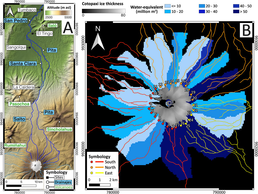
Figure 1. (A) Cotopaxi’s northern drainage network and main locations for references. (B) Total water-equivalent volume (WEV) at each basin according to Van Wyk de Vries et al. (2022), and source locations every 500 m to each drainage system: South (red), North (orange) and East (yellow). Modified from Vasconez et al. (2024).

2 Case study

Cotopaxi (0.677°S, 78.436°W, 5,897 masl) is an active glacier-clad volcano (Hall et al., 2008; Hidalgo et al., 2024) in Ecuador’s Eastern Cordillera, located 60 km southeast of Quito (Ecuador’s capital with a population of ∼2.7 million) and 40 km south of Sangolqui with a population of ∼97,000 (Figure 1A). Its glacier covers 9.71 km², with an average thicknesses of 47 ± 7 m (Figure 1B), holding an estimated volume of 450 ± 100 million m³ (Van Wyk de Vries et al., 2022). Cotopaxi’s cone-shaped structure channels meltwater and lahars into three main drainage systems: the Cutuchi River to the South, the Tambo-Tamboyaku Rivers to the East, and the Pita-San Pedro Rivers to the North, with the potential to impact communities such as Latacunga, Sangolqui and Tumbaco, and critical infrastructure, along these paths (Figure 1A). The last major lahar event occurred on 26 June 1877 when an explosive eruption generated a 14 km asl ash column and pyroclastic density currents (PDCs), triggering lahars that devasted areas along the volcano’s drainage network. Over 400 lives and thousands of livestock were lost, and significant infrastructure damage occurred, especially in Latacunga city towards the South of the volcano (Sodiro, 1877; Wolf, 1878). Recent expert elicitation estimates a 30%–40% probability of a 1877-type eruption during the next century (Tadini et al., 2021). Such an event could generate lahars capable of long-distance devastation, threatening lives, infrastructure, and livelihoods far from the volcano, as witnessed in historical times.

In this study, we focus on lahars flowing through Cotopaxi’s northern drainage system. The Salto River originates on the northwestern flank of Cotopaxi and flows along the base of the inactive neighbouring Rumiñahui volcano, while the Pita River begins in the northeast and drains at the base of the inactive Sincholahua volcano (Figure 1A). These two rivers merge 22 km downstream near the inactive Pasochoa volcano, continuing as Pita River. Approximately, 3.5 km further down, the Santa Clara River originates on the eastern slopes of Pasochoa (Figure 1A). Historical records (Sodiro, 1877; Wolf, 1878) and geological evidence (Mothes et al., 2004, 2016a) indicate that Cotopaxi lahars have overtopped from the Pita into the Santa Clara River at “La Caldera” site, 25 km away from Cotopaxi volcano. This region is marked by waterfalls and narrow canyons, 40–100 m deep and 40–180 m wide (Vasconez et al., 2024). About 20 km downstream, the Pita and Santa Clara Rivers converge to form the San Pedro River, which flows along the base of the inactive Ilalo volcano (Figure 1A) before joining larger rivers and eventually reaching the Pacific Ocean after a ∼280 km journey.

3 Data

Most of the data used in this study is derived from the findings in our earlier manuscript (Vasconez et al., 2024), which incorporated historical reports, fieldwork campaigns, hazard maps and published research spanning the past four decades. Below, we summarize the source conditions (scenario), topographic data, and the mathematical/physical simulator used to describe the flow dynamics.

3.1 Source conditions (scenario)

Vasconez et al. (2024) assigned peak discharges to source locations based on results of previous studies (Mothes et al., 2004) and the weighted volume of water present in Cotopaxi’s current glacier (Van Wyk de Vries et al., 2022). This approach determined a maximum peak discharge of 22,500 m³/s for sources located within the basin displaying the highest water-equivalent volume (WEV) (Vasconez et al., 2024), which is the maximum amount of water that could potentially be released by the current glacier within each basin surrounding the volcano (Van Wyk de Vries et al., 2022). As a result, 27 distinct sources were identified across the glacier (Figure 1B), with 9 of them (Source 12 to Source 20, see Table 1) draining into the northern drainage (Vasconez et al., 2024). Multiple source locations may fall within the same basin, leading to identical peak discharge values. For instance, Sources 18 through 20 share the same basin, each with a peak discharge of 16,154 m³/s (Table 1; Figure 1B). Notably, none of the northern sources reach the maximum peak discharge of 22,500 m³/s, as the highest WEV is found in the southeastern basins, which feed the eastern drainages (Figure 1B). Using a triangular hydrograph and an assumed 15-minutes duration (Table 1), peak discharge values can be converted into volumes for each source, allowing for the calculation of the cumulative volume of water delivered to each main drainage system. As a result, the northern drainages receive 34.8 million m³ (Table 1), which accounts for the 28.7% of the total water released in the 1877-type scenario, equivalent to 121 million m³ (Vasconez et al., 2024).

Table 1

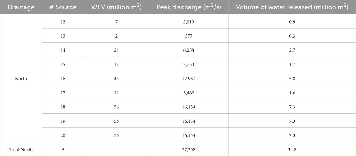
Table 1. Maximum peak discharge for each source location on the northern drainage network based on weighted water-equivalent volume (WEV) reported in Van Wyk de Vries et al. (2022), and a triangular hydrograph whose maximum expected peak discharge occurs at 2.5 min and lasts 15 min (Vasconez et al., 2024).

3.2 Cotopaxi’s DEM

For Cotopaxi volcano, three local DEMs have been produced in the last 20 years: a 30-meter DEM built from digitised topographic maps in 2006 (Souris, 2006), a 4-meter DEM constructed by SIGTIERRAS in 2010, and a 3-meter DEM delivered by the Instituto Geográfico Militar in 2015. In this study, we used the 3-meter DEM which covers the entire volcanic edifice and its main drainages. This DEM was used in our earlier paper to extract the main drainage network and then to generate perpendicular cross-sections along it, to calculate the minimum channel width (Vasconez et al., 2024). These cross-sections, 240 for the northern drainage, were spaced at 1,000-m intervals and extended over a length of 1,000 meters, based on the assumption that the maximum gully width in the study area is less than this distance. As a result, Vasconez et al. (2024) found that a 6-meter resolution DEM fully (100%) represents the actual topography of Cotopaxi’s northern drainage network, when assuming a “V” shape for the narrowest ravines (19 m width, i.e., 6 × 3 = 18 m), while a 15-m DEM captures 91.25% and a 30-m DEM only 55.8% of the drainage network.

3.3 Mathematical/physical simulator

For the present study, the simulator used was Kestrel (Langham and Woodhouse, 2024), which solves the shallow layer equations for liquid and solid phases over topography (DEM), including parameterizations for erosion and deposition of sediment and the corresponding morphodynamic changes. These processes alter the solid content during flow, and the simulator incorporates a novel drag formulation that adjusts between a turbulent fluid (low solid concentration) and a granular flow (high solid concentration) as the flow propagates over time (Langham and Woodhouse, 2024; Phillips et al., 2024). Kestrel is a generalised of a long-established shallow layer morphodynamic code called LaharFlow (Woodhouse et al., 2016), which was calibrated for volcanic debris flows (lahars) and made freely available via a web interface (accessible at this link). LaharFlow has been widely used for hazard assessment by national agencies and by academics, with over 200 users in 20 countries. Kestrel and LaharFlow were developed by the University of Bristol (UK) and is freely available at this link. Kestrel requires the domain and source locations to be specified, and the source properties were assigned in this study as follow: source radius (set to 100 m), hydrograph (peak discharge at 2.5 min vs. time fixed at 15 min) and simulation time (2.5 h). Additionally, physical parameters are necessary for simulator closures that account for specific physical processes (Table 2). For this study, we use the default parameter values calibrated for lahar applications presented at this link, as adopted by Woodhouse et al. (2016), Phillips et al. (2024) and Vasconez et al. (2024). Our simulations were conducted on a server with an AMD EPYC 7551P 32-Core Processor and 125 GB of RAM, running in serial mode on a single CPU at 2 GHz. This setup enables initiated multiple simulations simultaneously in parallel (high-throughput computing), with each utilizing its own CPU in serial mode, optimizing resource use while maintaining consistent performance across runs. This configuration is useful in practical hazard assessment as it allows multiple uncertain scenarios to be computed in parallel. Simulations were configured to produce results every 3 min of flow advancement, leading to a total of 50 outputs files per DEM, along with an additional file storing the maximum recorded values for the entire simulation.

Table 2

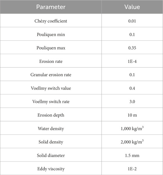
Table 2. Kestrel parameters with values calibrated for lahars (Woodhouse et al., 2016).

4 Methodology

Our study assesses two key issues: (i) the topographical changes resulting from DEM upscaling, and (ii) the differences in outcome predictions when using upscaled DEMs to simulate lahars with the dynamic simulator Kestrel. To analyse topographic changes, we use the 3-meter DEM as the reference. For the simulation comparisons, we base our evaluation on predictions derived from the 10-meter upscaled DEM. It is important to note that we do not perform simulations using the original 3-meter DEM due to its prohibitively high computational cost, estimated to require years of processing time for our case study. All analyses are conducted for the 1877 Cotopaxi lahar scenario, focusing specifically on the complex northern drainage system.

4.1 Impact of DEM resolution on topographic detail

Running dynamic lahar simulations in serial on a 3-m DEM poses a significant computational challenge, with estimated runtimes reaching approximately 1 year using the available 2 GHz processor. To address this limitation, resampling techniques can be applied to increase pixel size, thereby reducing computational demands at the potential expense of simulation fidelity (Stevens et al., 2002; Sulis et al., 2011).

In this study, we resample the 3-m DEM to resolutions of 10-, 15-, 20- and 30-meters. We utilized bilinear interpolation as it is widely adopted for DEM resampling because it efficiently produces smooth, continuous surfaces while minimizing stair-step artifacts which is critical for terrain analysis where abrupt discontinuities can introduce errors (Racoviteanu et al., 2007; Burrough et al., 2015). Additionally, this method is the default interpolation technique in-built into the Kestrel simulator.

To evaluate the impact of upscaling on terrain representation, we employed 240 cross sections from Vasconez et al. (2024) to extract topographic profiles from the 3-m DEM and each upscaled DEM. Profile extraction was performed using the “Profile Tool” plugin in QGIS. These extracted profiles were compared both visually and quantitatively to assess deviations from the 3-meter DEM. Three key metrics were calculated: minimum and maximum altitude deviations, and the area under the profile. Altitude deviations were computed by comparing the minimum and maximum values from each resampled DEM profile to the corresponding minimum and maximum elevations in the original 3-m DEM. The area under the profile was computed by summing the product of segment distances (equal to DEM resolution) and corresponding altitudes in meters above sea level (m asl). The percentage difference in area was then quantified relative to the 3-meter DEM. For example, in the case of the 10 m DEM, the relative difference in area is calculated as: (Area_10m – Area_3m)/Area_3m.

4.2 Quantifying differences in simulation predictions across upscaled DEMs

We perform simulations of the lahar dynamics using the upscaled 10, 15, 20 and 30 m resolution DEMs. The model cell resolution was fixed to be equal to the DEM resolution. At the model output time steps and at each transect location, the model simulations are compared to the 10 m resolution reference simulation (15, 20, 30 m–10 m/10 m). The quantities of interest predicted by the model include inundation area, maximum flow depth and speed, maximum runout distance, among others. Additionally, we record and compare the elapsed computation time and resulting files size.

4.2.1 Propagation disparities at 15-minute time intervals

To assess the influence of DEM resolution on lahar dynamics, results were extracted at 15-minute intervals in each simulation (10-, 15-, 20- and 30-meter DEMs), yielding a total of 10-time steps per simulation. At each time step, the inundation area was calculated to evaluate the spatial evolution of the lahar extent over time. Inundation areas were calculated in QGIS by creating binary masks for each output raster, where pixels were classified as inundated areas (1) and no data (0). This approach ensured a consistent and systematic assessment of lahar extent across different DEM resolutions.

One of the default Kestrel outputs is a raster file denoted as “inundation time”, which represents the first time that any cell in the domain is inundated by the flow. This inundation time output file was analysed to derive two key parameters: Maximum Inundation Distance and Propagation Speed. The Maximum inundation Distance is defined as the farthest downstream extent reached by the lahar at fixed time intervals and provides insight into how DEM resolution influences lahar runout predictions. The maximum inundation distance was measured at 15-minute intervals along Pita-San Pedro River system, which represents the primary lahar flow path (Figure 1A). The Propagation Speed is calculated as the average speed at which the lahar front advanced downstream using the maximum inundation distance. Comparing propagation speeds across different DEM resolutions is one way to quantify how terrain representation affects predictions of lahar mobility and flow dynamics.

4.2.2 Maximum depth, speed and solid fraction differences

During simulation, the Kestrel simulator generates and updates a file that contains the maximum values of various physical parameters (regardless of the specific time at which they occur). We performed detailed comparisons of the results from the resampled DEMs for maximum depth, speed and solid fraction, by extracting key metrics such as mean, standard deviation and maximum values for each parameter across the entire inundated area. Additionally, we plotted the results for visual comparison, focusing on critical areas like the maximum inundation distance and overtopping zones. Finally, using the drainage network derived from the 3-meter DEM, we extracted the maximum depth and speed along the Pita-San Pedro thalweg (Figure 1A) to explore the differences in the main river channel across the various DEM resolutions outcomes.

4.2.3 Normalized root mean square error and inundation detector

To quantify pixel-by-pixel differences between simulation results, we applied two complementary approaches: the Normalized Root Mean Square Error (NRMSE) method and an Inundation Detector on the maximum file results. Both techniques used the 10-m DEM simulation as the reference to compare against the coarser 15-, 20- and 30-meters predictions. Two Python scripts for these analyses are available in this link. To ensure consistent evaluation, we first downscaled the coarser DEM simulation results to 10-m resolution using bilinear interpolation for NRMSE and nearest neighbour interpolation for the Inundation detector. This enabled direct pixel-by-pixel comparisons across all DEMs.

NRMSE is a metric that evaluates simulation accuracy by comparing predicted values to observed values while normalizing the error for interpretability. In this study, we applied the NRMSE to maximum flow depth, speed, solid fraction and impact pressure, the eroded depth and inundation time, in areas where both the reference and each coarser DEM had overlapping data. This approach prevents overestimations of error caused by resolution-driven differences in inundation area, which would arise if the entire simulated extent were considered.

To complement the NRMSE analysis, we implemented an Inundation Detector, which evaluates discrepancies across the entire simulated inundation area, including non-overlapping zones. We first generated binary inundation masks from the maximum inundation extent, assigning a value of one to inundated areas and zero to non-inundated zones. The 10-m simulation results were used as the reference to categorize pixels as follows: (i) “true positives” if pixels were inundated in both the 10-m and coarser DEM simulations; (ii) “false negatives” if pixels were inundated in the 10-DEM but not in the coarser DEMs; and (iii) “false positives” if pixels were inundated in the coarser DEMs but not in the 10 m DEM.

This combined approach ensures a comprehensive evaluation of DEM resolution impacts on simulation predictions, with the NRMSE quantifying physical-variable differences in overlapping areas and the Inundation Detector capturing discrepancies in overall inundation extent.

4.2.4 Computational performance

Since all simulations were carried out on the same server, we were able to assess computational performance in terms of the time required to advance through one percentage of the simulation (out of 100%) and the total time needed to complete the 150-minutes run in our study. Additionally, we evaluated the cumulative size of the resulting files, in our case 50 output files generated at 3-minute intervals, plus the file containing the maximum values. Importantly, all output files were written in NetCDF (.nc) format by Kestrel and were subsequently utilized for this analysis.

4.3 Assessing potential lahar damage from simulations

The current Cotopaxi lahar hazard maps delineate hazard zones using binary classification, identifying areas as either “at risk” or “safe” (Mothes et al., 2016b, 2016a). While this approach helps local stakeholders recognize general danger zones, it lacks quantitative hazard data within these areas. As a result, these maps do not support detailed risk assessments, making it difficult to categorize hazard levels, evaluate potential damage to infrastructure, and prioritize mitigation efforts effectively. Our simulations aim to bridge this gap towards detailed hazard assessment, but their fidelity is influenced by DEM resolution. To illustrate this effect, we conducted a preliminary analysis of potential lahar-induced building damage using hazard zones derived from our simulations. Although this analysis is not the primary focus of this study, it offers a valuable reference for future research and applied risk evaluations. In particular, our DEMs are digital topographic maps that have removed surface features including buildings. Therefore, we cannot compute impacts on buildings directly, but instead use our computed quantities as proxies for potential damage scales. We assume that buildings within these zones are subjected to an impact pressure calculated as the sum of hydrostatic and the hydrodynamic pressures, as is commonly assumed (e.g., Chehade et al., 2021) and used as an indicator of potential building damage. By mapping this parameter from our simulation results, we provide a preliminary, practical, spatially explicit approach to evaluate lahar damage levels across different areas.

To achieve this, we employed the impact pressure equation (Equation 1) proposed by Chehade et al. (2021) and utilized in our previous study Vasconez et al. (2024), which is defined as:

$P_{impact}=\left(C\left({\rho }_{solid}-{\rho }_{water}\right)+{\rho }_{water}\right)\left({gh+V}^2\right)(1)$

where C is the maximum solid fraction, ρ_solid is the solid density (2,000 kg/m³), ρ_water is the water density (1,000 kg/m³), g is gravitational acceleration (9.81 m/s²), h is the maximum depth (m) and V is the maximum speed (m/s).

The impact pressure is then categorized using the thresholds proposed by Zanchetta et al. (2004), which provide a framework to define the following damage levels: pressures exceeding 3 kPa can break a wooden door, pressures between 3 and 35 kPa may cause moderate damage, from 35 to 90 kPa can result in severe damage, and pressures over 90 kPa could lead to complete destruction of reinforced concrete structures. While these thresholds offer a useful reference for evaluating lahar damage, they may not precisely correspond to the structural characteristics of buildings in our study area. Additionally, the exact physical properties of these buildings remain unknown, introducing some uncertainty into the damage assessment (Vasconez et al., 2024). Consequently, these results are intended as a reference to forecast potential damage in the event of a future 1877-type lahar scenario at Cotopaxi.

The buildings to be exposed was established by creating a 700-meter lateral buffer around the official lahar hazard zone for the northern drainage area (Mothes et al., 2016a). The buffer polygon was used instead of the exact hazard polygon to account for the differences between our simulation results and the official maps, ensuring no potential at-risk structures were overlooked. We then extracted the buildings by intersecting the buffer polygon with the data from the Google Maps Open Buildings database yielding a total of 77,176 buildings within the lahar hazard zone and buffer area. Importantly, the influence of the buildings’ planimetric area (90 m² on average for the study area) versus the pixel size of the simulation predictions (i.e., 100-, 225-, 400- and 900-m²) was not accounted in this analysis, as buildings were represented as centroids regardless of their actual shape and footprint. Consequently, the number of buildings and percentages presented in this investigation serve as broad indicator of exposure at different damage levels. We are using number of buildings as a metric of the different extents of damage that arise due to DEM resolution, rather than computing the pressures that buildings would actually experience.

5 Results

The results of this study are organized according to the structure outlined in the Methodology section, focusing on topographical changes and differences in model predictions.

5.1 Topographical changes after resampling the 3-meter DEM

Figure 2 shows examples of cross sections along a 14 km length of Pita River between 3,500 and 2,500 m asl. The figure illustrates the thalweg, fixed at 500 m (dashed light-blue line), which represents half of the maximum length of the cross-sectional profiles. Additionally, two light-blue lines are placed 56 m on each side of the thalweg to represent the average width of the gullies for the northern drainage network, which totals 112 m (Vasconez et al., 2024). Topographic changes are minimal where the black and the coloured lines overlap, with differences increasing as the two lines diverge. At first sight, the divergence becomes more pronounced as pixel size increases, with the largest differences observed between the 3- and 30-m DEMs and the smallest between the 3- and 10-meter DEMs. This highlights that upscaling the 3-meter DEM not only modifies the topography but may also affects the location of the thalweg, with these effects intensifying as the pixel size increases.

Figure 2

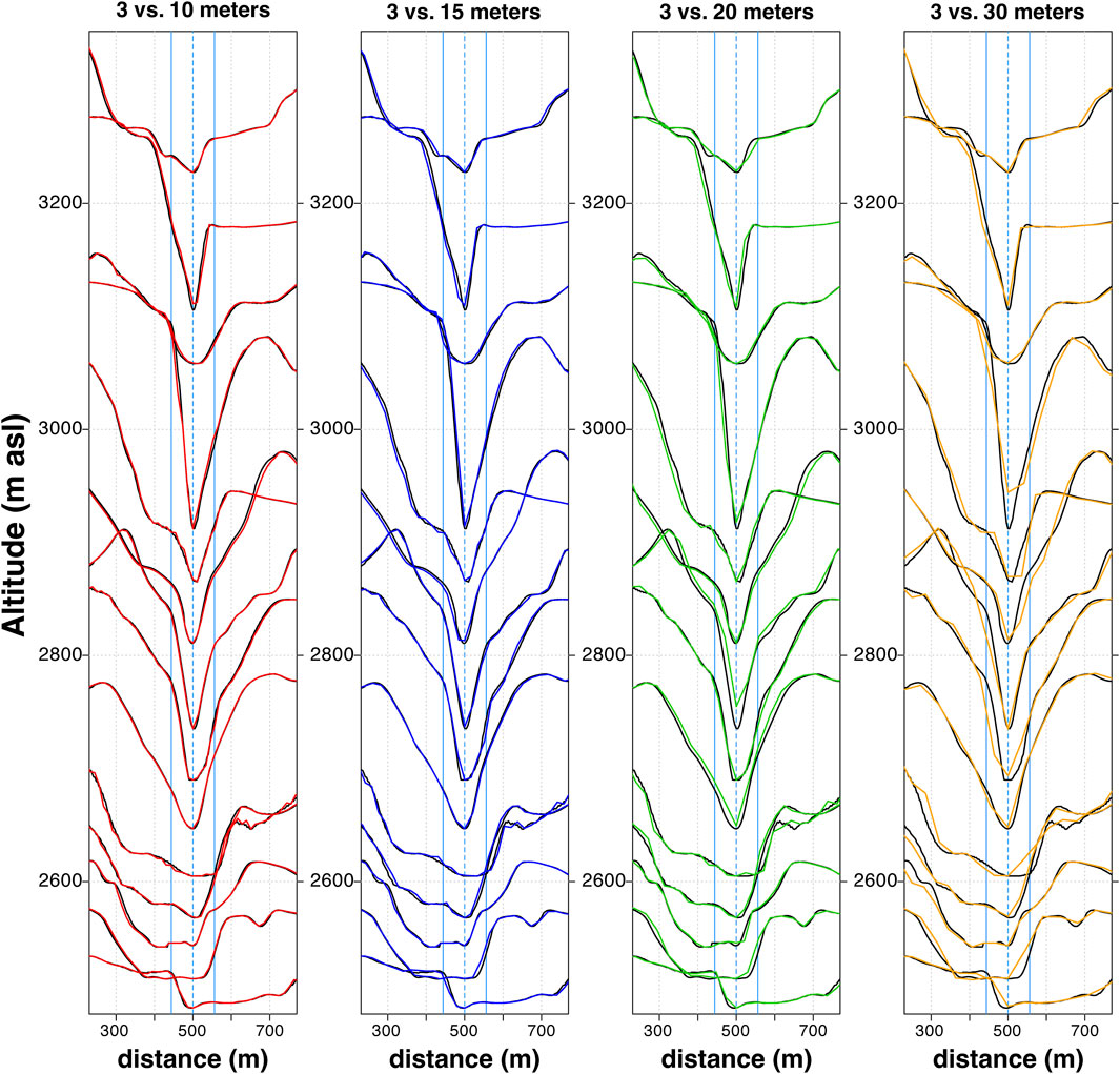
Figure 2. Cross-sections along Pita River. The black line represents the profile obtained from the 3-meter DEM, while the red, blue, green, and orange lines correspond to profiles derived from the 10-, 15-, 20- and 30-meter DEMs, respectively. The light-blue dashed line marks the thalweg, with additional light-blue lines indicating the average gully width based on Vasconez et al. (2024) for Cotopaxi’s northern drainage network.

Beyond the visual discrepancies, we quantify the differences of the minimum and maximum altitudes, as well as the area beneath each profile, using the 3-m DEM as the reference dataset (Figure 3). A total of 3,600 values (i.e., 3 variables for 240 profiles across 5 DEM resolutions) were compared for each parameter (Supplementary Data Sheet S1). Figure 3A shows the percentage difference in area under the profiles, revealing that the area increases by up to 4% as the pixel size grows. In other words, this indicates that with largest pixel sizes, the area above the profile, representing inundation sections, decreases. Additionally, comparing the minimum and maximum altitudes across each profile (Figures 3B,C), we observed that as pixel size increases, the minimum altitude tends to increase and the difference may rise by up to 30 meters, while the maximum altitude decreases, and the difference may reach up to 10 m. This indicates that the ravines become progressively shallower as the pixel size increases. These changes are more pronounced in the 20- and 30-meter DEMs, whereas the 10- and 15- meter DEMs show smaller differences in all evaluated parameters (Figure 3). DEM upscaling directly changes topography, which may ultimately produce changes in the debris flow simulation predictions, as analysed in Section 5.2 and 6.1.

Figure 3

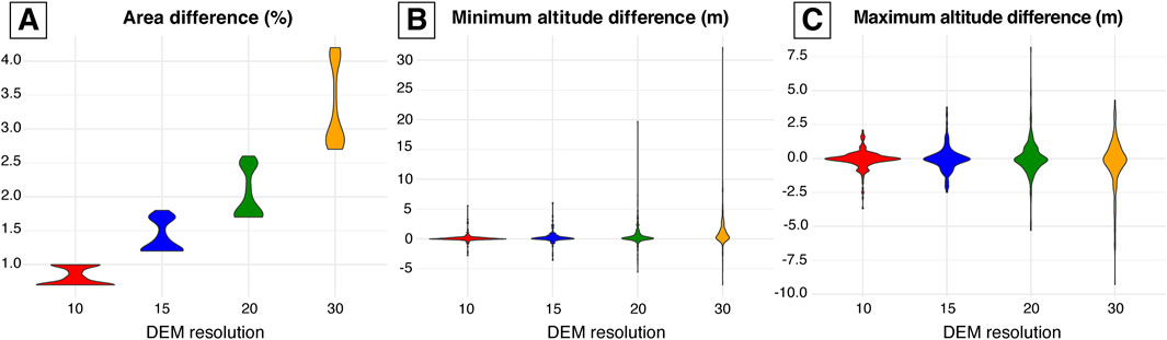
Figure 3. Violin plots illustrating the differences between the upscaled DEMs and the 3-meter DEM for: (A) the percentage difference in the area under the profile, (B) the minimum altitude, and (C) maximum altitude in meters.

5.2 Differences in simulation predictions

5.2.1 Inundation area, maximum inundation distance and propagation speed at time-intervals

Figure 4 illustrates the differences in simulation predictions at 15-minute intervals for inundation area, maximum inundation distance, and derived propagation speed. Overall, both inundation area and maximum inundation distance increase as simulation advances, while propagation speed decreases. The largest inundation area of 154 km² is obtained with the 30-meter DEM, whereas the smallest (98 km²) is associated with the 10-meter DEM (Figure 4A). Notably, the difference in inundation area between these two DEMs reaches a significant 58%. In contrast, the maximum inundation distance is achieved with the 15-meter DEM simulation at 70.5 km, while the 30-m DEM results in the shortest distance of 66.2 km (Figure 4B). The results from the 10- and 20-meter DEMs closely align with the 15-m prediction, reaching 70.4 km and 69.2 km, respectively, which represents a maximum differential of −1.6%. These findings show that the 30-meter DEM indeed underestimates the inundation extent. This inverse relationship, where a larger inundation area corresponds to a shorter inundation distance, reflects the impact of DEM upscaling on topographical smoothing (Figures 2, 3), which redistributes the volume over a broader area, thereby reducing its reach (see discussion section 6.1).

Figure 4

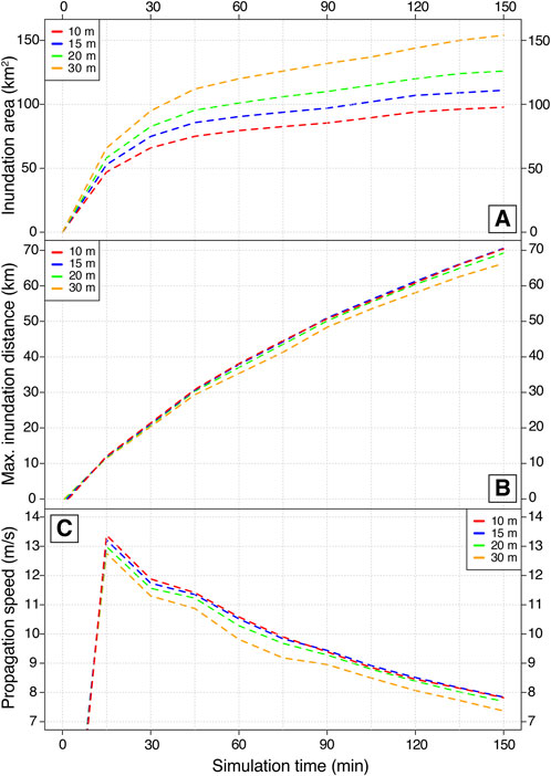
Figure 4. Model predictions at 15-minute intervals for: (A) Inundation area, (B) Maximum inundation distance, and (C) Propagation speed shown for the 10, 15, 20 and 30-meter DEMs represented by red, blue, green and orange dashed lines, respectively.

For propagation speed, there is a sharp initial increase due to the shape of the hydrograph, which releases most of the material early on, combined with the steep topography at the volcanic edifice during the first kilometres. After this initial surge, propagation speed gradually decreases, as elevation gradient decreases. Overall, propagation speed ranges from 7.4 to 13.4 m/s (Figure 4C), values consistent with those observed in similar events (Pierson, 1985; Pierson et al., 1990). The highest speeds are produced with the 10- and 15-m DEMs, while the 30-m DEM yields the lowest values, yet the differences are less than −5% among all resolutions. Both maximum inundation distance and propagation speed, which are derived from the same information, show relatively small differences across the various DEMs, suggesting that these parameters can be estimated with reasonable confidence despite DEM resolution changes (Figures 4B,C). In contrast, inundation area exhibits much larger variability (up to 58%), indicating that this parameter is more sensitive to DEM resolution under the topographical conditions of our case study (Figure 4A).

5.2.2 Maximum depth, speed and solid fraction

When analysing the maximums result files, we observed that both maximum depth and speed decrease as the pixel size increases, while maximum solid fraction shows an opposite trend, increasing with coarse DEMs (Table 3). For the entire inundated area, the average maximum depth ranges from 1.5 m (10-m DEM) to 0.8 m (30-m DEM), reflecting a 47.1% reduction. The standard deviations (std) of the maximum depths between these two extremes differ by −38.5%, and the overall maximum depth is reduced by −62.5%. A similar pattern is observed for maximum speed, where the maximum shows a −81.3% difference, the average a −29.8% difference, and std a −24.0% difference between the 10-m and 30-m DEMs. Conversely, the solid fraction behaves differently, with the average showing a 16.3% difference, indicating that the 30-m DEM results contain a higher particle concentration compared to the 10-m DEM (Table 3). Notably, the maximum solid fraction value remains constant at 0.64 (64% solid fraction) due to model’s closures for granular debris flows, as is the case for lahars (Woodhouse et al., 2016).

Table 3

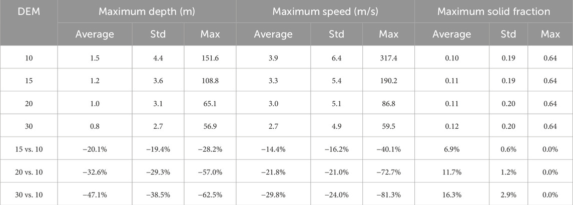
Table 3. Average, standard deviation (std), and maximum values (over space) for the temporal maximum depth, speed, and solid fraction recorded at any time for the 10-, 15-, 20- and 30-meter resolution DEMs. The table also includes the corresponding differences (±%) when compared with the results from the 10-m DEM.

Figure 5 shows the maximum depth of the lahar across the same geographic region derived from simulations using different DEM resolutions. The colour scale, ranging from blue to red, represents the lahar’s maximum depth, with red areas indicating deeper flows (>5 m), usually occurring in canyons, and blue areas representing shallower flows that appears on plains. Figure 5 enables a general visual comparison of the flow distribution and inundation patterns predicted by the model as DEMs resolution is upscaled. Inundation extends across the terrain, with notable variations in width and flow paths depending on the spatial resolution used. For example, the higher resolution (10-meter) reveals more detailed and finer flow patterns, while coarser 30-m DEM presents a smoother and broader distribution of the lahar. As reported in section 5.2.1, increasing the pixel size leads to a larger inundation area, while the maximum inundation distance slightly decreases as indicated by the black dashed line in Figure 5 and discussed in Section 6.1.

Figure 5

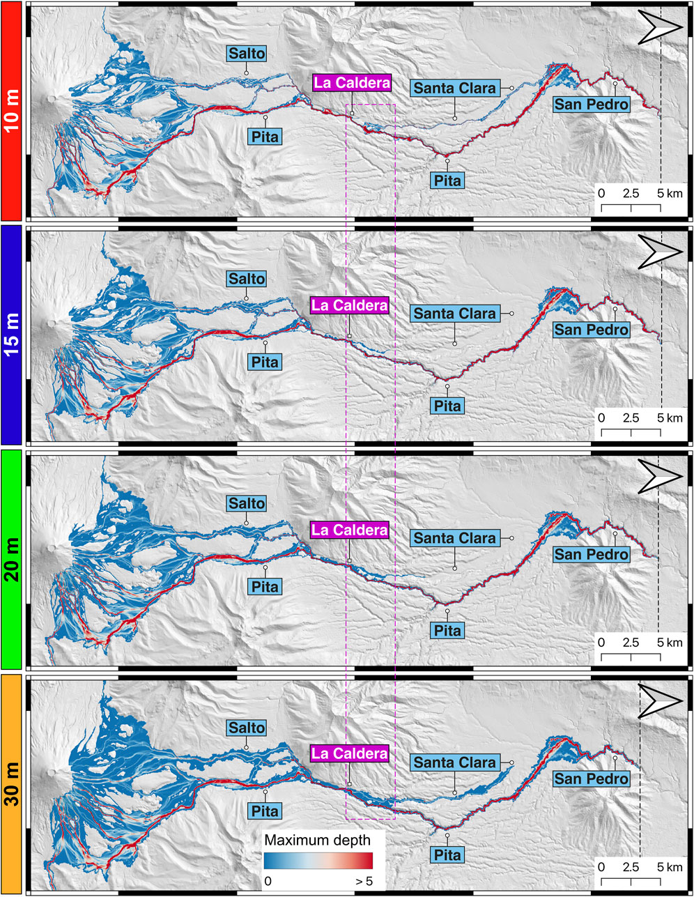
Figure 5. Maximum depth predictions for simulations on 10-, 15-, 20- and 30- meter DEMs visually comparing flow distribution and inundation patterns. The black dashed line depicts the maximum inundation distance, while the purple dashed polygon outlines the area where overtopping could occur. Note the discrepancies in Santa Clara River.

Figure 5 also allows for a detailed comparison of the model-predicted inundation patterns. The Pita River is the main drainage on Cotopaxi’s northern flank of meltwater from the glacier, but historical lahars have overtopped from the Pita channel to the Santa Clara River (Figures 1A, 5). All our results, regardless of the DEM resolution, captured the overtopping process with varying spread (Figure 5). For instance, the simulations on 10- and 30-meter DEMs both predict substantial overflow into the Santa Clara River compared to the 15- and 20-meter results. However, the 10- and 30-meter predictions differ in the extent and location of the overtopping zone. In the 10-meter simulation, a smaller lahar overflow occurs at La Caldera site due to multiple lahar fronts arriving at the same spot at different times, while the main overflow occurs about 1 km downstream from La Caldera (Figure 5). In contrast, the 30-m simulation predicts overtopping as one continuous zone from La Caldera site to ∼4 km downstream (Figure 5). Interestingly, the 15- and 20-meter DEM simulations suggest smaller amounts of overtopping at La Caldera, and the Santa Clara flows apparently stop before reaching residential areas, after 150 min simulation time (Figure 5). These differences are significant because the overtopping process substantially increases the exposure of residential areas downstream, around Sangolqui (Figure 1), impacting the potential mitigation measures that can be considered for the Santa Clara drainage (see section 6.1).

We extracted and compared the maximum depth and speed along Pita-San Pedro thalwegs, as shown in Figure 6. Overall, both maximum flow depth and speed decrease as pixel size increases, with the largest differences observed between the 10- and 30-meter DEMs. The average maximum depth along the Pita-San Pedro Rivers ranges from 16.7 to 12.6 m (Figure 6A), which represents a −24.6% difference. For maximum speed, average ranges between 12.1 and 11.7 m/s, which corresponds to a difference of −3.3% (Figure 6A). For maximum depth, the most significant outlier appears in the 15-m simulation results at 104.3 meters, but aside from this, a decreasing trend is evident as pixel size increases (Figure 6A) and is shown clearly by the mean values. A similar behaviour is observed for maximum speed. The highest value for both depth and speed along the river are predicted for the higher-resolution DEMs, and these values decrease as the DEMs become coarser (Figure 6B). These changes can also be linked to shifts in riverbed location due to resampling during interpolation, as noted in section 5.1. This further emphasizes the impact of DEM resolution on topography and simulation results (see Section 6.3), particularly in how it influences physical-parameter predictions along thalwegs which are the most impacted regions during lahar transit.

Figure 6

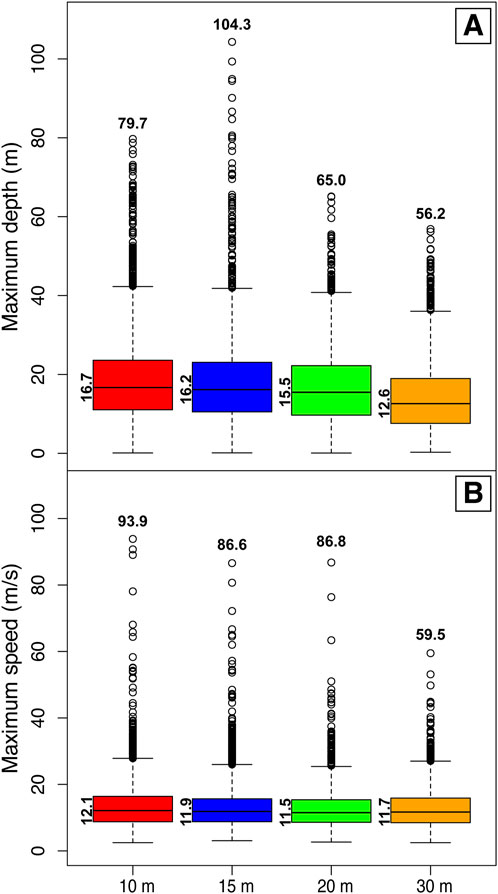
Figure 6. Boxplot along Pita-San Pedro thalwegs showing differences in (A) maximum depth and (B) maximum speed with values compared across different DEM resolutions.

5.2.3 Normalized Root Mean Square Error (NRMSE) and Inundation Detector

NRMSE values for maximum depth range from 1.23% for the 15-m simulation to 1.82% for the 30-m simulation, indicating a progressive increase in error with coarser resolutions (Figure 7A). Similarly, for maximum speed, NRMSE values range from 0.88% (15-m) to 1.31% (30-m) (Figure 7A). Maximum solid fraction exhibits greater variation, with NRMSE values from 24.23% to 40.23%, the lowest observed for the 15 m simulation. The derived maximum impact pressure fluctuates between 0.43% and 0.54%, showing minimal discrepancy (0.1%) between the 15-m and the 30-meter simulations (Figure 7A). Maximum erosion increases from 3.08% (15-m) to 5.19% (30-m), while inundation time varies from 15.18% (15-m) to 19.89% (30-m, Figure 7A). Overall, percentage differences relative to the 10-m predictions remain small but tend to increase with coarser resolutions. The largest discrepancies occur between the 10- and 30-m simulations, particularly for the maximum solid fraction and inundation time (Figure 7A).

Figure 7

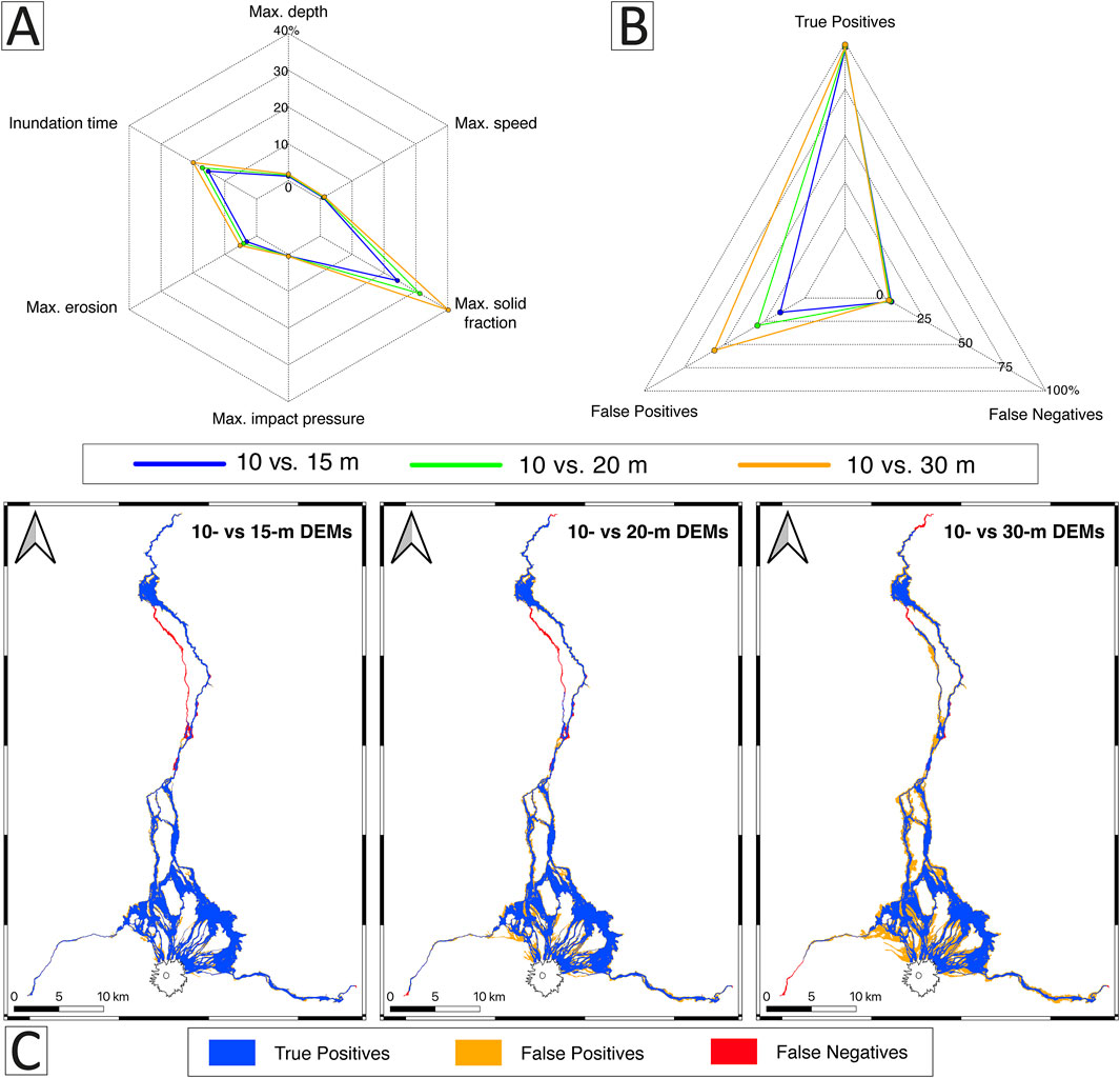
Figure 7. Radar charts illustrating the impact of DEM resolution on lahar predictions. (A) Comparison of six physical variables at pixel-scale using NRMSE, considering only areas where the 10-m and coarse DEM results overlap. (B) Comparison of inundated pixels across the entire inundation area, using the 10-m result as reference. (C) Resulting maps from the Inundation Detector, blue areas highlight true positives, orange false positives and red false negatives.

To quantify the discrepancy in inundated area, we applied the Inundation Detector, using the 10-m DEM results as reference. This approach categorizes pixels into true positives, false negatives and false positives. True positives: pixels where both reference and predictions match, varying from 96.1% to 97.69% (Figure 7B). False negatives or pixels inundated in the reference raster but absent in the predictions (3.82%–2.3%) and false positives or pixels inundated in the prediction raster but absent in the reference (15.33%–56.32%, Figure 7B). Results suggest that most of inundated pixels coincide across resolutions, with minor discrepancies in critical areas like La Caldera, where overtopping complexity influences flow paths and maximum inundation distance (Figures 5, 7C). Additionally, false positives increase with pixel size as inundation extent spreads laterally (Figures 4A, 5, 7B,C).

5.2.4 Computational performance

Simulation performance was evaluated based on processing time per output, total computing time, and cumulative file size. Results show that coarse DEM resolutions substantially improve computational efficiency. The 10-m DEM required an average 1.5 ± 1 day per output and a total of 77.4 days to complete the simulation, while the 30-m DEM completed the same simulation in just 2.2 days, a 97.2% reduction in total time. File sizes followed a similar trend, with the 10-m DEM producing 5.6 GB of data, compared to only 0.9 GB for the 30-m DEM (an 82.1% reduction). These results demonstrate that DEM upscaling significantly reduces computational demands, emphasizing the trade-off between computational feasibility and resolution-dependent accuracy in lahar hazard modelling.

6 Discussion

6.1 Effect of DEM resolution on lahar volume distribution: challenges at “La Caldera” site

Predictions of the inundation area and maximum inundation distance are strongly controlled by the topographic data resolutions (Stevens et al., 2002; Huggel et al., 2008). Larger pixel sizes smooth out or obscure topographic features, such as small channels or obstacles, so they cannot be resolved in the model simulations (Rocha et al., 2022). This can lead to a more generalized flow path where inundation extends into broader areas that would not be affected at a higher resolution (Figures 5, 7C). In gravity-driven flow models, the direction and speed of the flow depends heavily on small variations in slope and topography (Figures 2–4, 6). Higher resolution DEMs capture these details more accurately, enabling a more precise channelization of the flow (Figure 5). Coarser resolutions, however, lack these details, causing the flow to spread more broadly and increasing the apparent inundation area (Figures 4, 5, 7C). Additionally, in models that do not account for erosion and deposition (e.g., LaharZ) coarser DEMs tend to significantly reduce maximum inundation distance due to volume conservation constraints (Stevens et al., 2002; Huggel et al., 2008). In contrast, when using simulators that incorporate erosion and deposition processes, as in our case, this reduction is much less pronounced. In coarser-resolution runs, increased erosion compensates for the loss of confinement (Table 3), helping to sustain the flow volume and maintain its downstream propagation (Figure 5). Regarding lateral volume distribution, the averaging effect of coarser resolutions promotes broader flow distribution, further exaggerating the apparent inundation extent (Figure 5).

These discrepancies become especially critical in complex topographies like Cotopaxi’s northern drainage network, where lahars have historically overflowed into pirate drainages, i.e., drainages that do not originate in Cotopaxi (Figure 5, Wolf, 1878; Mothes et al., 2004). Such overtopping significantly increases the risk to populations and infrastructure (Aguilera et al., 2004). Previous numerical simulations have captured this phenomenon (Aguilera et al., 2004; Frimberger et al., 2021; Vasconez et al., 2024), as do the results of this study, although with varying degrees of inundation extent, even though we utilized the same lahar-scenario and physical-based simulator (Figure 5).

To test our results, we conducted two approaches: a drone survey to assess potential overtopping areas under current topographic conditions, and a detailed field campaign to locate historical lahar deposits. Both activities focused on La Caldera area (purple dashed polygon in Figures 5, 8A), where the Pita River is characterized by deep canyons with multiple waterfalls. The drone survey provided a high-resolution orthophoto (16.5 cm) and a video simulating the lahar’s flow perspective. From the video, we identified three critical areas where overtopping could potentially occur (Figure 8A), characterized by displaying lower elevations and narrow sections along the Pita River (see Supplementary Video S1). Using the orthophoto and the simulation results, we pinpointed these three key areas for focused fieldwork (Figure 8A). At La Caldera site, we identify at least three recent lahar deposits (Figure 8B), confirming that overtopping has occurred here despite a currently 60-meter altitude difference between the Pita thalweg and the Santa Clara River headwaters. This finding aligns with both geological and historical evidence of overflow at this location (Figures 8A,B). However, lahar deposits thickness is about 1 m (Figure 8B) which seems relatively thin for flows that reportedly devastated Sangolqui, located 14–20 km downstream (Mothes et al., 2004; Figure 1A). Approximately 1.2 km downstream from La Caldera, we found an ancient cemented volcanic breccia (Figure 8C) within an area designated as a lahar hazard zone in the current hazard map (Mothes et al., 2016a). Interestingly, neither our 10-m simulation nor the outcrops in this area indicate evidence of past lahars (Figures 8A,C). However, the 15-, 20- and 30-m simulations predict inundation in this area. This may suggest that faster-moving lahars did not leave deposits, or that upstream overflow at La Caldera was minimal, as observed in the field. About 250 m downstream from the volcanic breccia, recent lahar deposits were found near a soccer field, marking a second overtopping site (Figure 8A; Supplementary Video S1). Beyond this point a small hill clearly separates the Santa Clara and Pita drainages (Figure 8A). Once past the hill, about 200-m downstream, there is another overtopping zone (Figure 8A; Supplementary Video S1) where recent lahar deposits are clearly visible, providing further evidence of historical flow pathways and overflow events at this area.

Figure 8

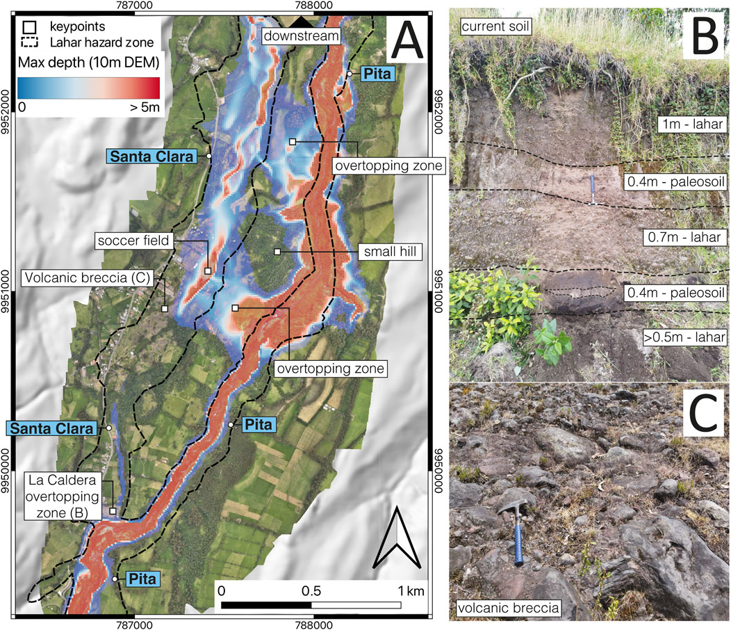
Figure 8. (A) Orthophoto of “La Caldera” area. The black dashed polygon outlines the lahar hazard zone defined by Mothes et al. (2016a), while the colour scale from red to blue represents the maximum lahar depth based on the 10-meter DEM simulation for reference. (B) Outcrop at the headwaters of Santa Clara River (La Caldera site), showing three recent lahar deposits interlayered with paleosoils. (C) Ancient cemented volcanic breccia observed within the lahar hazard zone.

When comparing our field observations with simulation results, we found that the 10- and 20-meter simulations align best with the field-observed overtopping patterns, as both identified the three critical overflow zones, albeit at different magnitudes (Figure 5). In contrast, the 30-m simulation combined those zones into one, while the 15-meter simulation only identified overtopping at La Caldera site (Figure 5). These overflow areas are significant as initial assessments exist to designing mitigation structures, such as dikes, for potential risk reduction strategies. Further research is needed to quantify uncertainties related to overflow behaviour across different scenarios and to assess the effectiveness of potential infrastructure, via numerical simulations, before investing in mitigation efforts. Our results suggest that this phenomenon is a more complex than previously assumed.

Our findings highlight the importance of topography selection in accurately determining lahar inundation extent and flow paths when using numerical models. For this study, we used a “V” shape representation (3 pixels wide) for the narrowest ravines. However, the observed differences between the 10- and 15-meter DEMs, which capture 97.08% and 91.25% of the 3-m DEM topography respectively, suggest that a 4- or 5-pixel width may be necessary for a more precise representation of complex terrain like U-shaped ravines. However, running simulations on high-resolution DEMs for long-distance lahars significantly increases computational time and resource demands, underscoring the need to balance the cost-benefit trade-off of using high-resolution DEMs to ensure reliable results within practical timeframes (see Section 6.3). Finally, as emphasized by Huggel et al. (2008), model outputs should not be interpreted as definitive boundaries but rather as indicators that distinguish between high-risk and safe areas. For critical locations like “La Caldera”, hazard zone delineation should not rely on a single DEM or scenario; rather, a probabilistic approach could be taken to incorporate sensitivity analysis and account for uncertainties in input data, as illustrated in this study.

6.2 A practical example of DEM resolution influence on assessing potential lahar damage

Depending on the simulation and DEM resolution, between 18.29% and 26.56% (Table 4) of the total buildings could experience any level of damage by lahars in the event of an 1877-type eruption. Specifically, we estimate 14,262 buildings impacted when using the 10-m DEM, 14,116 with the 15-m DEM, 16,195 with the 20-m DEM, and 20,495 buildings with the 30-m DEM. These results are in agreement with previous analysis (see Section 5.2), with coarser resolutions (i.e. 30-m DEM) generally indicating a larger inundation area, and therefore a larger number of potentially damaged structures. Table 4 shows the proportions of buildings in each of the damage categories from Zanchetta et al. (2004) when using different simulation resolutions. As an example, between 1,200 and 1,423 buildings are within the complete damage areas, computed from the 30- and 15-m model predictions, respectively. The largest discrepancy occurred in the low-damage category (<3 kPa), where the 30-m simulation results produced an approximately double count of impacted buildings compared with the other model resolutions (Table 4). For other damage levels, differences across model resolutions were negligible (around 0.26%). These findings underscore that the overestimation of inundated areas with coarse DEMs mainly affects low-damage zones, while predictions from moderate to complete damage levels remain consistent across DEM resolutions (Table 4). However, we note that our DEMs do not include features of the urban landscape, which require a high-resolution (meter to sub-meter) scale DEM to resolve.

Table 4

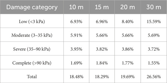
Table 4. Percentage of the number of buildings (from the Google Map Open Buildings database) within each damage category, classified according to Zanchetta et al.’s, thresholds. The total of 77,176 buildings represents 100%, encompassing structures within the official lahar hazard zone (Mothes et al., 2016a) and a 700-meter lateral buffer.

Figure 9 provides a close-up of the most densely populated area within Cotopaxi’s northern drainage, highlighting the variation in damage categories across different DEM predictions. In each case, zones of complete destruction (i.e., highest impact pressure) are concentrated near the river, particularly along Pita River, while damage levels gradually decrease with distance from the channels. Notably, the 10- and 30-m DEMs predict inundation of the Santa Clara River (Figure 5), exposing buildings overlooked with the 15- and 20-meter simulations. Additionally, the 30-m DEM extends the inundation area laterally, thereby increasing the number of buildings located inside the low-damage level zone (Figure 9; Table 4). Although the overall percentage distribution of damage categories may appear similar across DEM predictions, the specific areas and buildings affected differ between resolutions (see Section 5.2.3). To better account for these differences, future studies should focus on developing probabilistic damage level maps. Such maps would incorporate a range of scenarios based on a probabilistic density function, and should be simulated with consideration of the necessary topographic detail as well as computational requirements. For the northern Cotopaxi drainage, our results recommend using the 10-m DEM as the optimal resolution for future ensemble approaches, which is also comparable to the 90 m² building footprint.

Figure 9

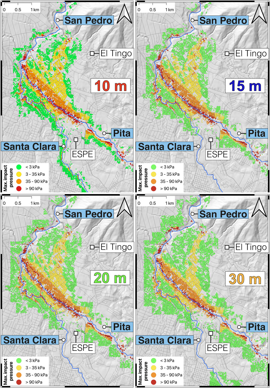
Figure 9. Damage level maps based on different DEM predictions showing expected building damage levels across impact pressure categories. Each building is represented by a centroid extracted from polygons in the Google Maps Open Building database. The colour scale ranges from green, indicating low damage, to red, indicating complete destruction based on the Zanchetta et al.’s categories.

6.3 Balancing costs and benefits of DEM upscaling when high-resolution DEMs are available

Numerical simulators that accurately capture lahar dynamics are crucial for hazard assessment and risk forecasting (Aguilera et al., 2004; Lupiano et al., 2021). Over time, these simulators have become increasingly sophisticated, often necessitating high-performance computing and extended processing times. Selecting an appropriate DEM resolution is essential to balance computational efficiency with the desired accuracy of flow representation. Generally, the highest feasible resolution for available data and computational resources yields the most precise flow path modelling, as model accuracy depends on both the robustness of the numerical approximations and the quality of the topographic dataset (Vaze et al., 2010; Rocha et al., 2022). Although higher DEM resolutions typically improved the accuracy of extracted morphometric features like watershed delineation and stream network, overly fine resolutions may introduce noise or artifacts, potentially leading to inaccurate flow paths and direction calculations due to micro-scale variations (Sulis et al., 2011; Dávila-Hernández et al., 2022; Rocha et al., 2022). Consequently, users must carefully balance these factors when selecting DEMs and simulators for gravity-driven flow models.

Our analysis provides a comprehensive view of how DEM resolution affects lahar model predictions, balancing computational efficiency with predictive fidelity. While simulations using the 30-m DEM results can produce outcomes within a few days, providing a broad overview of the inundation area, these tend to overestimate the extent and underestimate the maximum inundation distance, maximum flow depth and speed (Table 3; Figures 4–7). This expanded inundation area may, in some circumstances, be beneficial for conservative hazard zoning, as it inherently accounts for uncertainties in potential future lahar sizes, making it valuable for identifying safe and hazard-prone zones. However, there may be features of the flow that are not well approximated in the low-resolution simulation, and the wider distribution of the flow may result in reduced depths in the channel, with a consequence on the flow dynamics. In our simulations, this effect is, to some extent, compensated by increased erosion that acts to maintain a high flow volume flux in the channel. In contrast, the 10-m DEM simulation yields more precise predictions of physical properties of the flow and deposits, which are essential for designing and locating mitigation infrastructure. It also captures the topography more accurately, resulting in improved flow path predictions and lateral spread. However, it is computational demands, up to months of processing (for our case study, in a serial implementation), make it impractical for rapid crisis response, though it is feasible during periods of volcanic quiescence.

Comparisons of physical flow properties, such as maximum depth and speed, reveal notable discrepancies depending on both the evaluation method and spatial domain. Using average-based metrics (Section 5.2.2) over the entire inundated area, differences can reach as high as −47.1%. In contrast, when using the NRMSE restricted to overlapping inundated areas (Section 5.2.3), discrepancies drop significantly to just 1.82%. This apparent contradiction arises because coarser DEMs yield broader inundation areas, which often include marginal zones with minimal flow depth and speed. These low values reduce the overall averages disproportionately, also reflected in impact pressure analyses (Section 6.2). When focusing on values along the main flow path, or applying NRMSE solely to common inundated zones, differences in maximum depth and speed are greatly reduced (Figures 6, 7). As a result, the most substantial discrepancies are concentrated in false positive areas, whereas true positives areas show far more consistent parameter estimates (Figure 7).

This consistency in overlapping areas is especially important for authorities, as it enables resource allocation and mitigation planning based on reliable data, particularly in moderate-to high-risk zones, thereby enhancing preparedness and resilience strategies. The detailed comparisons of DEM resolutions presented in this study lays the groundwork for future ensemble-based modelling approaches that incorporate scenario variability and assist in evaluating the effectiveness of proposed mitigation measures.

6.4 Local vs. global DEMs: implications for lahar hazard modelling

Globally, 1,281 volcanoes have erupted during the Holocene, with approximately 57% of these located in low- or middle-income countries (World Bank, 2023; Global Volcanism Program and Venzke, 2024). Additionally, increasing population growth has led to human settlement in moderately to highly hazardous volcanic areas, contributing to an overall rise in volcanic risk worldwide (ISDR, 2004). As a result, many volcanoes have become hazardous but lack adequate monitoring systems and hazard maps. For those volcanoes with hazard maps, 63% were created solely using geologic history, while only 17% incorporated both geologic data and numerical simulations (Calder et al., 2015). Challenges to effective gravity-driven flow modelling in volcanic regions include the limited availability of local DEMs, particularly for remote or developing regions (Huggel et al., 2008). In response, global initiatives have focused on creating widely accessible DEMs, such as SRTM, ALOS and ASTER, which are free available through online platforms like Open Topography.

We simulated our scenario using the 30-m SRTM DEM and compared its results with those from the upscaled 30-m DEM. Figure 10 represents a visual comparison of maximum inundation extent and distance, using maximum depth predictions as a reference. Overall, the SRTM-based simulation reveals markedly different inundation patterns and lahar behaviour compared to the local upscaled 30-m DEM (Figure 10). For instance, in the SRTM simulation, the lahar in Pita River stopped after flowing only 3 km downstream from La Caldera site, while in the Santa Clara River, it extended up to 9 km (the maximum inundation distance for the entire simulation; Figure 10A). In contrast, the upscaled 30-m DEM predicted a much great inundation distance, with the Pita River lahar reaching 37 km downstream and the Santa Clara lahar extending 17 km downstream from La Caldera site (Figure 10B). The SRTM simulation exhibits an inundation pattern characterised by localised regions of high depth (see inset in Figure 10A), contrasting sharply with the more continuously-varying depths observed in simulations using the local DEM (Figures 5, 10B). This “spotted” pattern may suggest inconsistencies in flow connectivity, likely due to limitations in the STRM DEM’s topographic representation. Notably, the SRTM-based simulation did not inundate residential areas, as the lahar terminated prematurely despite a fixed 2.5-hour simulation duration. This indicates that the SRTM DEM may underestimate average flow propagation speed, highlighting the challenges in capturing topographic details crucial for lahar modelling in this region.

Figure 10

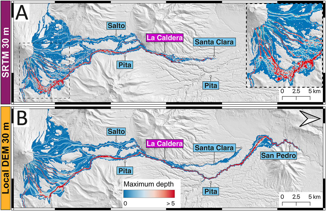
Figure 10. Maximum depth predictions based on (A) global 30-m SRTM DEM and (B) local upscaled 30-m DEM, illustrating differences in flow distribution and inundation patterns. The inset in panel (A) provides a close-up of the northeastern flank of Cotopaxi cone, highlighting the “spotted” inundation pattern observed in the SRTM-based predictions. Note that North arrow points to the right.

Previous studies have compared lahar simulation predictions using DEMs from free global sources, such as SRTM and ASTER, with DEMs derived from digitised topographic maps (Stevens et al., 2002; Huggel et al., 2008; Castruccio and Clavero, 2015). Generally, digitised topographic maps have produced more accurate results than global DEMs, as they better capture terrain features and lack errors associated with sensor geometry and canopy cover (Stevens et al., 2002; Castruccio and Clavero, 2015). Similar limitations of global DEMs have been noted in urban flood modelling, where their use has led to reduced accuracy in hydrodynamic simulations (Zandsalimi et al., 2024). Common issues include low vertical and spatial resolution, vegetation artifacts, temporal inconsistencies, and the impact of void-filling algorithms (Saksena and Merwade, 2015; Aristizabal et al., 2024; Nandam and Patel, 2024; Zandsalimi et al., 2024, 2025). Our findings underscore the value of using local, high resolution DEMs for lahar hazard mapping. While global DEMs like SRTM are readily available, modelling users should be cautions of their inherent limitations, as these can lead to inaccuracies in the prediction of gravity-driven hazards.

7 Conclusion

This study provides a comprehensive perspective of how DEM resolution influences topographic representation and consequently, lahar simulation outcomes, highlighting the balance between computational efficiency and predictive fidelity. Each DEM resolution offers distinct benefits depending on the intended application and user requirements. The 30-m DEM can generate results relatively quickly, providing a broad overview of inundation areas. However, it tends to overestimate inundation extents and underestimate maximum inundation distance and key physical properties of the flow. Conversely, the 10-m DEM offers more detailed predictions for flow dynamics and physical parameters, which are essential for designing and positioning mitigation infrastructure. However, the longer computing time suggests it is less suitable for immediate crisis response but remains a very valuable tool for long term planning and detailed risk assessments. Notably, overestimation of inundated areas in coarse DEMs produces additional regions of low-depth and slower moving flow which artificially inflate the extent of low-damage regions. However, predictions of regions of moderate to complete damage remain consistent across simulations with different DEM resolutions. This consistency allows authorities to reliably zone and prioritize resources and mitigation efforts in areas at risk of moderate to complete damage, regardless of the DEM resolution used in simulations.

Our results also illustrate that complex features of lahar dynamics, such the over-topping of flow into the Santa Clara River, are only captured when detailed topographic data is used. This can have a critical impact on hazard assessment, as overtopping increases residential exposure and influences the decision making of potential sites for mitigation infrastructure in our case study. Importantly, our coarse resolution DEMs are generated by upscaling higher resolution DEM, and results are significantly more variable if the coarse resolution DEM is obtained from global datasets due to inherent inconsistencies. Field observations confirmed repeated lahar overtopping at the La Caldera site in the past centuries, despite a 60-meter altitude difference between the Pita River thalweg and the Santa Clara River headwaters, in concordance with historical reports. However, both fieldwork and simulations show that overtopping has also occurred in other locations, only a few kilometres downstream from La Caldera site, which suggests that this is a more complex process than previously assumed.

Overall, our findings offer a foundational framework for optimizing lahar hazard simulations using high-resolution DEMs over extensive areas. Although the substantial computational demands of dynamic-based simulators currently constrain their use in real-time applications, this study highlights several promising avenues for improvement. These range from relatively straightforward measures such as selecting appropriate topographic representations, to more advanced approaches, including parallelizing computational workflows, automatic grid refinement, leveraging GPU-accelerated processing, and integrating surrogate or deep learning models to accelerate simulations without compromising accuracy. Such advancements will be essential for delivering timely and reliable lahar hazard assessments in complex terrains and ultimately for enabling ensemble simulations within a probabilistic framework.

Data availability statement

The raw data supporting the conclusion of this article will be made available by the authors, without undue reservation. Kestrel is available for free on https://kestrel-unibristol.readthedocs.io/en/latest/index.html, https://github.com/jakelangham/kestrel/ and the LaharFlow webtool on https://www.laharflow.bristol.ac.uk/.

Author contributions

FV: Conceptualization, Data curation, Formal Analysis, Investigation, Methodology, Validation, Visualization, Writing – original draft, Writing – review and editing. JP: Formal Analysis, Funding acquisition, Investigation, Project administration, Resources, Supervision, Validation, Writing – review and editing. SA: Formal Analysis, Funding acquisition, Investigation, Project administration, Resources, Supervision, Validation, Writing – review and editing. MW: Investigation, Resources, Software, Supervision, Validation, Writing – review and editing.

Funding

The author(s) declare that financial support was received for the research and/or publication of this article. This work was supported by the UKRI GCRF under grant NE/S009000/1, Tomorrow’s Cities Hub.

Acknowledgments

We extend special thanks to the late Minard L. Hall, whose founding of IG-EPN was driven by his deep concern over the risk of a potential lahar-forming eruption at Cotopaxi. His vision and commitment significantly advanced Ecuadorian volcanology, raising awareness among decision-makers about the catastrophic impacts of such events. We are also sincerely grateful to Anais Vásconez Müller and Benjamin Bernard for their generous contribution in conducting the drone survey, which enabled the creation of the video and high-resolution orthophoto that enrich part of our discussion. Special acknowledgement is extended to Scott Watson for sharing the Google Earth Engine script that allowed us to extract building data from the Google Maps Open Building database. We thank Juan Anzieta for suggesting the Inundation Detector methodology which complemented the Goodness-of-fit evaluation. Additionally, we express our appreciation to the Kestrel team for their significant improvements to the code, which played a crucial role in this study.

Conflict of interest

The authors declare that the research was conducted in the absence of any commercial or financial relationships that could be construed as a potential conflict of interest.

Generative AI statement

The author(s) declare that Generative AI was used in the creation of this manuscript. Generative AI was used to enhance the writing of the first draft since the first author is not a native English-speaker. Afterwards, the manuscript was reviewed and edited by the coauthors, which is the submitted version.

Publisher’s note

All claims expressed in this article are solely those of the authors and do not necessarily represent those of their affiliated organizations, or those of the publisher, the editors and the reviewers. Any product that may be evaluated in this article, or claim that may be made by its manufacturer, is not guaranteed or endorsed by the publisher.

Supplementary material

The Supplementary Material for this article can be found online at: https://www.frontiersin.org/articles/10.3389/feart.2025.1611579/full#supplementary-material

SUPPLEMENTARY VIDEO S1Video simulating the lahar’s flow perspective at La Caldera region.

References

Aguilera, E., Pareschi, M. T., Rosi, M., and Zanchetta, G. (2004). Risk from lahars in the northern valleys of Cotopaxi volcano (Ecuador). Nat. Hazards 33, 161–189. doi:10.1023/B:NHAZ.0000037037.03155.23

CrossRef Full Text | Google Scholar

Aristizabal, F., Chegini, T., Petrochenkov, G., Salas, F., and Judge, J. (2024). Effects of high-quality elevation data and explanatory variables on the accuracy of flood inundation mapping via Height above Nearest Drainage. Hydrology Earth Syst. Sci. 28, 1287–1315. doi:10.5194/hess-28-1287-2024

CrossRef Full Text | Google Scholar

Auker, M. R., Sparks, R. S. J., Siebert, L., Crosweller, H. S., and Ewert, J. (2013). A statistical analysis of the global historical volcanic fatalities record. J. Appl. Volcanol. 2, 2. doi:10.1186/2191-5040-2-2

CrossRef Full Text | Google Scholar

Azizian, A., and Brocca, L. (2020). Determining the best remotely sensed DEM for flood inundation mapping in data sparse regions. Int. J. Remote Sens. 41, 1884–1906. doi:10.1080/01431161.2019.1677968

CrossRef Full Text | Google Scholar

Blong, R. (2000). “Volcanic hazards and risk management,” in Encyclopedia of volcanoes (Academic Press), 1215–1227. Available online at: https://www.elsevier.com/books/encyclopedia-of-volcanoes/sigurdsson/978-0-08-054798-5. (Accessed November 3, 2024)

Google Scholar

Burrough, P. A., McDonnell, R. A., and Lloyd, C. D. (2015). Principles of geographical information systems. Third. USA: Oxford University Press. Available online at: https://books.google.com/books?hl=es&lr=&id=kvoJCAAAQBAJ&oi=fnd&pg=PP1&dq=Principles+of+Geographical+Information+Systems+Burrough,+P.+A.,+%26+McDonnell,+R.+A.+(1998)&ots=aME6cgz7JE&sig=8lZqMXnVGiUQAQ0M8KSVXXy-L-o (Accessed May 9, 2025).

Google Scholar

Calder, E., Wagner, K., and Ogburn, S. (2015). “Volcanic hazard maps,” in Global volcanic hazards and risk (Cambridge University Press Cambridge), 335–342. Available online at: https://books.google.com/books?hl=es&lr=&id=8loZCgAAQBAJ&oi=fnd&pg=PA335&dq=hazard+maps+volcanoes&ots=eOq14RtOzn&sig=tR4V46qLxSdONg3MaBS9w9iyZag (Accessed November 7, 2024).

CrossRef Full Text | Google Scholar

Capra, L., Poblete, M. A., and Alvarado, R. (2004). The 1997 and 2001 lahars of Popocatépetl volcano (Central Mexico): textural and sedimentological constraints on their origin and hazards. J. Volcanol. Geotherm. Res. 131, 351–369. doi:10.1016/S0377-0273(03)00413-X

CrossRef Full Text | Google Scholar

Castruccio, A., and Clavero, J. (2015). Lahar simulation at active volcanoes of the Southern Andes: implications for hazard assessment. Nat. Hazards 77, 693–716. doi:10.1007/s11069-015-1617-x

CrossRef Full Text | Google Scholar

Chehade, R., Chevalier, B., Dedecker, F., Breul, P., and Thouret, J.-C. (2021). Discrete modelling of debris flows for evaluating impacts on structures. Bull. Eng. Geol. Environ. 80, 6629–6645. doi:10.1007/s10064-021-02278-3

CrossRef Full Text | Google Scholar

Dávila-Hernández, S., González-Trinidad, J., Júnez-Ferreira, H. E., Bautista-Capetillo, C. F., Morales De Ávila, H., Cázares Escareño, J., et al. (2022). Effects of the digital elevation model and hydrological processing algorithms on the geomorphological parameterization. Water 14, 2363. doi:10.3390/w14152363

CrossRef Full Text | Google Scholar

Frimberger, T., Andrade, S. D., Weber, S., and Krautblatter, M. (2021). Modelling future lahars controlled by different volcanic eruption scenarios at Cotopaxi (Ecuador) calibrated with the massively destructive 1877 lahar. Earth Surf. Process. Landforms 46, 680–700. doi:10.1002/esp.5056

CrossRef Full Text | Google Scholar

Global Volcanism Program Venzke, E. (2024). Volcanoes of the world, 5.2.0. doi:10.5479/si.GVP.VOTW5-2024.5.2

CrossRef Full Text | Google Scholar

Goulden, T., Hopkinson, C., Jamieson, R., and Sterling, S. (2016). Sensitivity of DEM, slope, aspect and watershed attributes to LiDAR measurement uncertainty. Remote Sens. Environ. 179, 23–35. doi:10.1016/j.rse.2016.03.005

CrossRef Full Text | Google Scholar

Hall, M. L., Samaniego, P., Le Pennec, J. L., and Johnson, J. B. (2008). Ecuadorian Andes volcanism: a review of Late Pliocene to present activity. J. Volcanol. Geotherm. Res. 176, 1–6. doi:10.1016/j.jvolgeores.2008.06.012

CrossRef Full Text | Google Scholar

Hengl, T. (2006). Finding the right pixel size. Comput. and Geosciences 32, 1283–1298. doi:10.1016/j.cageo.2005.11.008

CrossRef Full Text | Google Scholar

Hidalgo, S., Bernard, B., Mothes, P., Ramos, C., Aguilar, J., Andrade, S. D., et al. (2024). Hazard assessment and monitoring of Ecuadorian volcanoes: challenges and progresses during four decades since IG-EPN foundation. Bull. Volcanol. 86, 4. doi:10.1007/s00445-023-01685-6

CrossRef Full Text | Google Scholar

Huggel, C., Kääb, A., Haeberli, W., and Krummenacher, B. (2003). Regional-scale GIS-models for assessment of hazards from glacier lake outbursts: evaluation and application in the Swiss Alps. Nat. Hazards Earth Syst. Sci. 3, 647–662. doi:10.5194/nhess-3-647-2003

CrossRef Full Text | Google Scholar

Huggel, C., Schneider, D., Miranda, P. J., Delgado Granados, H., and Kääb, A. (2008). Evaluation of ASTER and SRTM DEM data for lahar modeling: a case study on lahars from Popocatépetl Volcano, Mexico. J. Volcanol. Geotherm. Res. 170, 99–110. doi:10.1016/j.jvolgeores.2007.09.005

CrossRef Full Text | Google Scholar

Hugonnet, R., Brun, F., Berthier, E., Dehecq, A., Mannerfelt, E. S., Eckert, N., et al. (2022). Uncertainty analysis of digital elevation models by spatial inference from stable terrain. IEEE J. Sel. Top. Appl. Earth Obs. Remote Sens. 15, 6456–6472. doi:10.1109/JSTARS.2022.3188922

CrossRef Full Text | Google Scholar

ISDR (2004). Living with risk: a global review of disaster reduction initiatives. United Nations Publications.

Google Scholar

Jiang, W., Yu, J., Wang, Q., and Yue, Q. (2022). Understanding the effects of digital elevation model resolution and building treatment for urban flood modelling. J. Hydrology Regional Stud. 42, 101122. doi:10.1016/j.ejrh.2022.101122

CrossRef Full Text | Google Scholar

Jones, R., Manville, V., and Andrade, D. (2015). Probabilistic analysis of rain-triggered lahar initiation at Tungurahua volcano. Bull. Volcanol. 77, 68. doi:10.1007/s00445-015-0946-7

CrossRef Full Text | Google Scholar

Laigle, D., and Bardou, E. (2021). “Mass-movement types and processes: flow-like mass movements, debris flows and Earth flows,” in Reference module in Earth systems and environmental sciences (Elsevier). doi:10.1016/B978-0-12-818234-5.00152-8

CrossRef Full Text | Google Scholar

Langham, J., and Woodhouse, M. J. (2024). The Kestrel software for simulations of morphodynamicEarth-surface flows. JOSS 9, 6079. doi:10.21105/joss.06079

CrossRef Full Text | Google Scholar

Lupiano, V., Catelan, P., Calidonna, C. R., Chidichimo, F., Crisci, G. M., Rago, V., et al. (2021). LLUNPIY simulations of the 1877 northward catastrophic lahars of Cotopaxi volcano (Ecuador) for a contribution to forecasting the hazards. Geosciences 11, 81. doi:10.3390/geosciences11020081

CrossRef Full Text | Google Scholar

Manville, V., Hodgson, K. A., and White, J. D. L. (1998). Rheological properties of a remobilised tephra lahar associated with the 1995 eruptions of Ruapehu volcano, New Zealand. N. Z. J. Geol. Geophys. 41, 157–164. doi:10.1080/00288306.1998.9514800

CrossRef Full Text | Google Scholar

Mead, S. R., and Magill, C. R. (2017). Probabilistic hazard modelling of rain-triggered lahars. J. Appl. Volcanol. 6, 8. doi:10.1186/s13617-017-0060-y

CrossRef Full Text | Google Scholar

Mothes, P., Espín, P., Hall, M., Vasconez, F., Sierra, D., and Andrade, S. D. (2016a). Mapa Regional de Amenazas potenciales del volcán Cotopaxi-Zona Norte. Available online at: https://drive.google.com/drive/folders/0B1GypW4co7KbZ0t5NER4OU1obzQ (Accessed July 13, 2024).

Google Scholar

Mothes, P., Espín, P., Hall, M., Vasconez, F., Sierra, D., Córdova, M., et al. (2016b). Mapa Regional de Amenazas potenciales del volcán Cotopaxi-Zona Sur. Available online at: https://drive.google.com/drive/folders/0B1GypW4co7KbZ0t5NER4OU1obzQ (Accessed July 13, 2024).

Google Scholar

Mothes, P., Hall, M. L., Andrade, D., Yepes, H., Pierson, T. C., Gorki Ruiz, A., et al. (2004). Character, stratigraphy and magnitude of historical lahars of Cotopaxi volcano (Ecuador). Acta vulcanol. 16, 1000–1023. doi:10.1400/19097

CrossRef Full Text | Google Scholar

Nandam, V., and Patel, P. L. (2024). A framework to assess suitability of global digital elevation models for hydrodynamic modelling in data scarce regions. J. hydrology 630, 130654. doi:10.1016/j.jhydrol.2024.130654

CrossRef Full Text | Google Scholar

Phillips, J., Barclay, J., Cole, P., Johnson, M., Miller, V., and Robertson, R. (2024). Impacts and prospective hazard analysis of rainfall-triggered lahars on St Vincent 2021–22. SP 539, 245–266. doi:10.1144/SP539-2022-313

CrossRef Full Text | Google Scholar

Pierson, T. C. (1985). Initiation and flow behavior of the 1980 pine creek and muddy river lahars, mount st. Helens, Washington. Geol. Soc. Am. Bull. 96, 1056–1069. doi:10.1130/0016-7606(1985)96<1056:iafbot>2.0.co;2

CrossRef Full Text | Google Scholar

Pierson, T. C., Janda, R. J., Thouret, J.-C., and Borrero, C. A. (1990). Perturbation and melting of snow and ice by the 13 November 1985 eruption of Nevado del Ruiz, Colombia, and consequent mobilization, flow and deposition of lahars. J. Volcanol. Geotherm. Res. 41, 17–66. doi:10.1016/0377-0273(90)90082-q

CrossRef Full Text | Google Scholar

Pistolesi, M., Cioni, R., Rosi, M., Cashman, K. V., Rossotti, A., and Aguilera, E. (2013). Evidence for lahar-triggering mechanisms in complex stratigraphic sequences: the post-twelfth century eruptive activity of Cotopaxi Volcano, Ecuador. Bull. Volcanol. 75, 698. doi:10.1007/s00445-013-0698-1

CrossRef Full Text | Google Scholar

Racoviteanu, A. E., Manley, W. F., Arnaud, Y., and Williams, M. W. (2007). Evaluating digital elevation models for glaciologic applications: an example from Nevado Coropuna, Peruvian Andes. Glob. Planet. Change 59, 110–125. doi:10.1016/j.gloplacha.2006.11.036

CrossRef Full Text | Google Scholar

Rocha, J., Duarte, A., Fabres, S., Quintela, A., and Serpa, D. (2022). Influence of DEM resolution on the hydrological responses of a Terraced catchment: an exploratory modelling approach. Remote Sens. 15, 169. doi:10.3390/rs15010169

CrossRef Full Text | Google Scholar

Saksena, S., and Merwade, V. (2015). Incorporating the effect of DEM resolution and accuracy for improved flood inundation mapping. J. Hydrology 530, 180–194. doi:10.1016/j.jhydrol.2015.09.069

CrossRef Full Text | Google Scholar

Schilling, S. P. (1998). LAHARZ; GIS programs for automated mapping of lahar-inundation hazard zones. U. S. Geol. Surv. Information Services [distributor]. Available online at: https://pubs.usgs.gov/of/1998/0638/report.pdf

Google Scholar

Sodiro, L. (1877). Relacion sobre la erupcion del Cotopaxi acaecida el dia 26 de junio de 1877. Imprenta Nacional. Available online at: https://repositorio.flacsoandes.edu.ec/handle/10469/12657 (Accessed May 16, 2024).

Google Scholar

Souris, M. (2006). Ecuador DEMs from digitized topographic maps (1:50000 and 1:100000). Available online at: http://www.savgis.org/ecuador.htm (Accessed December 29, 2023).

Google Scholar

Stevens, N. F., Manville, V., and Heron, D. W. (2002). The sensitivity of a volcanic flow model to digital elevation model accuracy: experiments with digitised map contours and interferometric SAR at Ruapehu and Taranaki volcanoes, New Zealand. J. Volcanol. Geotherm. Res. 119, 89–105. doi:10.1016/S0377-0273(02)00307-4

CrossRef Full Text | Google Scholar

Sulis, M., Paniconi, C., and Camporese, M. (2011). Impact of grid resolution on the integrated and distributed response of a coupled surface–subsurface hydrological model for the des Anglais catchment, Quebec. Hydrol. Process. 25, 1853–1865. doi:10.1002/hyp.7941

CrossRef Full Text | Google Scholar

Tadini, A., Roche, O., Samaniego, P., Azzaoui, N., Bevilacqua, A., Guillin, A., et al. (2021). Eruption type probability and eruption source parameters at Cotopaxi and Guagua Pichincha volcanoes (Ecuador) with uncertainty quantification. Bull. Volcanol. 83, 35. doi:10.1007/s00445-021-01458-z

CrossRef Full Text | Google Scholar

Thouret, J.-C., Antoine, S., Magill, C., and Ollier, C. (2020). Lahars and debris flows: characteristics and impacts. Earth-Science Rev. 201, 103003. doi:10.1016/j.earscirev.2019.103003

CrossRef Full Text | Google Scholar

Uesawa, S. (2014). A study of the Taisho lahar generated by the 1926 eruption of Tokachidake Volcano, central Hokkaido, Japan, and implications for the generation of cohesive lahars. J. Volcanol. Geotherm. Res. 270, 23–34. doi:10.1016/j.jvolgeores.2013.11.002

CrossRef Full Text | Google Scholar

Vallance, J. W. (2005). “Volcanic debris flows,” in Debris-flow hazards and related phenomena (Springer), 247–274.

Google Scholar

Vallance, J. W. (2024). “Lahars: origins, behavior and hazards,” in Advances in debris-flow science and practice. Editors M. Jakob, S. McDougall, and P. Santi (Cham: Springer International Publishing), 347–382. doi:10.1007/978-3-031-48691-3_12

CrossRef Full Text | Google Scholar

Van Wyk de Vries, M., Carchipulla-Morales, D., Wickert, A. D., and Minaya, V. G. (2022). Glacier thickness and ice volume of the Northern Andes. Sci. Data 9, 342. doi:10.1038/s41597-022-01446-8

CrossRef Full Text | Google Scholar

Vasconez, F. J., Phillips, J., Woodhouse, M. J., and Andrade, S. D. (2024). Numerical simulation of long-distance debris flows (lahars) on glacier-clad volcanoes: the case of Cotopaxi, Ecuador. Front. Earth Sci. 12, 1–21. doi:10.3389/feart.2024.1426088

CrossRef Full Text | Google Scholar

Vaze, J., Teng, J., and Spencer, G. (2010). Impact of DEM accuracy and resolution on topographic indices. Environ. Model. and Softw. 25, 1086–1098. doi:10.1016/j.envsoft.2010.03.014

CrossRef Full Text | Google Scholar

Viotto, S., Toyos, G., and Bookhagen, B. (2023). An assessment of the effects of DEM quality and spatial resolution on a model for mapping lahar inundation areas at volcán Copahue (Argentina and Chile). J. S. Am. Earth Sci. 121, 104138. doi:10.1016/j.jsames.2022.104138

CrossRef Full Text | Google Scholar

Wolf, T. (1878). Memoria sobre el Cotopaxi y su última erupcion, acaecida el 26 de junio de 1877, por Teodoro Wolf: Con una lámina y una carta topográfica. Imp. del comercio. Available online at: https://archive.org/details/memoriasobreelco00wolf/page/2/mode/2up (Accessed March 14, 2024)

Google Scholar

Woodhouse, M., Hogg, A., Phillips, J., Espín Bedón, P., Almeida, S., and Andrade, D. (2016). A model of lahars for hazard assessment. (Puerto Varas Chile). doi:10.13140/RG.2.2.35597.95201

CrossRef Full Text | Google Scholar

World Bank (2023). New World Bank country classifications by income level: 2022-2023. World Bank Blogs. Available online at: https://blogs.worldbank.org/en/opendata/new-world-bank-country-classifications-income-level-2022-2023 (Accessed November 7, 2024).

Google Scholar

Zanchetta, G., Sulpizio, R., Pareschi, M. T., Leoni, F. M., and Santacroce, R. (2004). Characteristics of May 5–6, 1998 volcaniclastic debris flows in the Sarno area (Campania, southern Italy): relationships to structural damage and hazard zonation. J. Volcanol. Geotherm. Res. 133, 377–393. doi:10.1016/S0377-0273(03)00409-8

CrossRef Full Text | Google Scholar

Zandsalimi, Z., Barbosa, S. A., Alemazkoor, N., Goodall, J. L., and Shafiee-Jood, M. (2025). Deep learning-based downscaling of global digital elevation models for enhanced urban flood modeling. J. Hydrology 653, 132687. doi:10.1016/j.jhydrol.2025.132687

CrossRef Full Text | Google Scholar

Zandsalimi, Z., Feizabadi, S., Yazdi, J., and Salehi Neyshabouri, S. A. A. (2024). Evaluating the impact of digital elevation models on urban flood modeling: a comprehensive analysis of flood inundation, hazard mapping, and damage estimation. Water Resour. Manage 38, 4243–4268. doi:10.1007/s11269-024-03862-4

CrossRef Full Text | Google Scholar