A high-precision and fast algorithm for three-dimensional magnetic anomalies on undulating terrain

This study addresses the challenge of efficiently and accurately computing three-dimensional undulating surface magnetic field data, which has become increasingly difficult with the development of airborne magnetic survey technologies. To solve this problem, we propose a new computational method that is both efficient and highly precise. This method utilizes a planar three-dimensional fast-forward algorithm to calculate multiple planar magnetic fields at different heights, followed by local continuation combined with trilinear interpolation to achieve an accurate conversion from planar magnetic fields to undulating surface magnetic fields. This enables the completion of three-dimensional high-precision fast forward calculations that can then be applied to the inversion algorithm to calculate the distribution of the three-dimensional magnetization rate. Multiple model examples were tested to verify the accuracy and efficiency of the proposed method.

1 Introduction

The magnetic method is a well-developed and widely applied geophysical exploration technique, with extensive use in mineral exploration, engineering geological surveying, geological mapping, and deep structural research (Prutkin and Saleh, 2009; Eppelbaum, 2011; Li and Oldenburg, 2010; David et al., 2019; Kirkby and Duan, 2019). Quantitative interpretation of magnetic anomalies faces challenges in the forward modeling and inversion of three-dimensional magnetic susceptibility models (Bhattacharyya, 1964; Bhattacharyya, 1980; Li and Oldenburg, 1996; Pilkington, 1997; Pilkington, 2008; Li and Sun, 2016; Liu et al., 2018). However, owing to the significant computational resource requirements, the efficiency of three-dimensional inversion is limited, which hampers its widespread application (Portniaguine and Zhdanov, 2000; Davis and Li, 2013; Rezaie et al., 2017).

Recently, researchers have proposed enhanced methodologies and targeted computational strategies to address this issue. When the observation point is situated on a regular grid in the plane, significant reductions in the computational and storage requirements can be achieved through equivalent calculations based on the symmetry of the geometric framework (Shengxian et al., 2018). Building on this foundation, further optimization algorithms have been developed by leveraging the fast Fourier Transform (FFT) to execute convolution operations in the spatial domain via multiplication operations in the frequency domain. These algorithms optimize both spatial computation accuracy and frequency-domain computation speed (Chen and Liu, 2019; Jing et al., 2019; Hogue et al., 2019; Yuan et al., 2022), enabling efficient and accurate three-dimensional forward and inversion computation.

When the observation point is situated on an undulating observation surface, the symmetry between the observation point and field source is disrupted, rendering direct utilization of the aforementioned algorithm unfeasible. To improve computational efficiency, Zheng et al. (2019) enhanced Parker’s formula in the wavenumber domain, achieving rapid and high-precision gravity forward modeling on undulating interfaces, as well as fast and accurate gravity forward simulation of density interface models with topography. In the spatial wavenumber domain, a numerical simulation algorithm for gravity anomalies based on an arbitrary Fourier transform using quadratic interpolation functions was developed; CPU-GPU acceleration was employed to further amplify the advantages of three-dimensional gravity anomaly forward modeling in this domain (Dai et al., 2024). In terms of spatial domain calculations, multiple planar fields encompassing undulating surfaces were computed using efficient algorithms for forward modeling. The forward field values at any given observation points are obtained by using local interpolation techniques (Li et al., 2018; Qiang et al., 2019). Although Li et al. (2018) utilized a cubic spline interpolation method capable of achieving a precise conversion from a planar magnetic field to an undulating surface magnetic field, its non-linear nature poses challenges when directly applied to three-dimensional linear inversion.

This study proposes a high-precision local linear interpolation method to address the aforementioned issues. This method initially employs physically meaningful local extrapolation for interpolation, subsequently enhancing the accuracy of interpolation through trilinear interpolation correction. Integrating this composite linear interpolation approach with a rapid algorithm for the magnetic field plane facilitates the efficient forward and inverse computations of large-scale aeromagnetic data.

2 Methods

2.1 Fast forward modeling algorithm for planar magnetic field

The underground space was assumed to be divided into $N_M\left(N_M=m\times n\times p\right)$ prism grid cells, where $m$ and $n$ represent the number of grid divisions in the north and east, respectively, and $p$ represents the number of grid divisions in the vertical direction. The observed magnetic field on the surface consisted of $N_{\Delta T}\left(N_{\Delta T}=m\times n\right)$ observation points, each corresponding to a horizontal position on the prism cell (Figure 1).

Figure 1

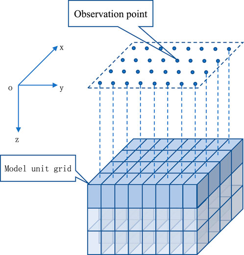
Figure 1. One-to-one correspondence between the spatial positions of the model unit grid and the measurement point grid.

According to the theory of magnetic field forward modeling, the forward process can be represented by a filtering formula (Equation 1) that balances the spatial domain accuracy and frequency domain speed in the forward calculation (Jing et al., 2019).

$\Delta \mathbf{T}=\mathbf{\text{VM}}={\mathbf{F}}^{-1}\left(\sum _{\mathit{k}=1}^{\mathit{p}}\mathbf{F}\left({\stackrel{\sim }{\mathbf{V}}}_{\mathit{k}}\right)·\mathbf{F}\left({\stackrel{\sim }{\mathbf{M}}}_{\mathit{k}}\right)\right),\left(1\le k\le p\right),(1)$

where vector $\Delta \mathbf{T}$ represents the forward modeling anomaly of the model with a dimension of $N_{\Delta T}$, $\mathbf{M}$ is the magnetization intensity according to the forward formula, also with a dimension of $N_M$, $\mathbf{V}$ represents the forward operator that connects observation data $\Delta \mathbf{T}$ and physical parameters $\mathbf{M}$, known as the forward coefficient matrix, which has a dimension of $N_{\Delta T}\times N_M$, $\mathbf{F}$ represents the fast Fourier transform in the positive direction while ${\mathbf{F}}^{-1}$ represents the fast Fourier transform in the inverse direction, ${\stackrel{\sim }{\mathbf{V}}}_{\mathit{k}}$ ($\left(2m-1\right)\times \left(2n-1\right)$)denotes the prism forward kernel matrix at depth k, and ${\stackrel{\sim }{\mathbf{M}}}_{\mathit{k}}$ ($\left(2m-1\right)\times \left(2n-1\right)$) refers to an extended matrix obtained by adding zeros to the magnetization intensity matrix at depth k. The symbol “∙” denotes the Hadamard product, representing element-wise multiplication between matrices of the same order. The derivation of Equation 1 is detailed in Supplementary Appendix A.

The first $m\times n$ elements in matrix ${\stackrel{\sim }{\mathbf{M}}}_{\mathit{k}}$ represent the density matrix elements of the kth layer in the model while the remaining elements are set to zero. The first $m\times n$ elements in matrix ${\stackrel{\sim }{\mathbf{V}}}_{\mathit{k}}$ correspond to the magnetic field response values at surface observation points for prism ${\stackrel{\sim }{\mathrm{M}}}_{m,n,k}$ with index number $\left(m,n\right)$ in the density matrix of the kth layer (with default starting index as 1). At this time, prism ${\stackrel{\sim }{\mathrm{M}}}_{m,n,k}$ has a density set to the unit magnetization intensity. The remaining elements in matrix ${\stackrel{\sim }{\mathbf{V}}}_{\mathit{k}}$ are stored symmetrically with respect to index number ${\stackrel{\sim }{\mathrm{M}}}_{m,n,k}$.

2.2 Fast forward algorithm for magnetic anomaly of undulating surfaces

To calculate the magnetic field at any point on the undulating surface, we adopted a systematic approach calculates the magnetic field distribution on multiple horizontal planes by using a fast algorithm and deriving observation point through a local interpolation technique. There are many local interpolation methods, such as local upward continuation, inverse distance-weighted interpolation, trilinear interpolation, Kriging interpolation, and cubic spline. If only the accuracy of forward modeling is considered, the nonlinear interpolation method may have a higher calculation accuracy. However, when forward calculation is used for linear inversion calculations, the interpolation method should be linear interpolation. In this study, a composite interpolation method that combines local continuation and trilinear interpolation was adopted. The specific steps were as follows. First, multiple horizontal planes (Figure 2) were selected as the calculation basis according to the terrain characteristics of the undulating observation surface. Multiple horizontal observation surfaces were arranged at equal intervals according to the longitudinal length of the underground space dissection grid. Such a setting enables the reuse of a large number of forward coefficient matrices, thereby saving considerable calculation time and storage space (Li et al., 2018).

Figure 2

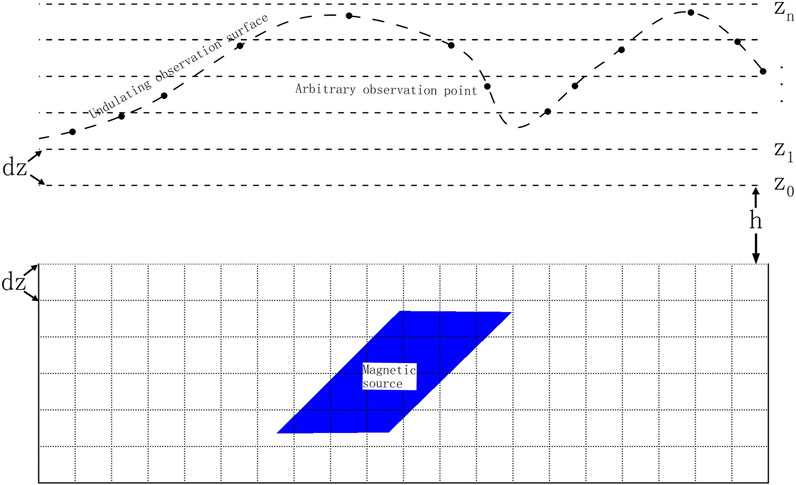
Figure 2. Schematic diagram of the relationship between the undulating observation surface and the horizontal observation surface.

An efficient three-dimensional magnetic field fast forward algorithm (Equation 1) was then used to perform the magnetic field forward calculation to obtain accurate magnetic field distribution data on these planes. The magnetic field calculation formula (Equation 2) for multiple horizontal planes is as follows:

$\mathbf{\Delta }{\mathbf{T}}_s={\mathbf{V}}_s\mathbf{M}(2)$

where vector $\mathbf{\Delta }{\mathbf{T}}_s$ represents the magnetic fields on the multiple horizontal observation planes and its dimension is $N_{\Delta Ts}\times 1$, i.e., the total number of observation points on multiple horizontal observation planes. Furthermore, ${\mathbf{V}}_s$ represents the forward coefficient matrix for calculating the magnetic field values of multiple horizontal observation planes, whose dimension is $N_{\Delta Ts}\times N_M$.

Finally, a high-precision local interpolation algorithm was adopted. The idea of the local interpolation algorithm (Equation 3) is as follows. First, the limited planar measuring points below the undulating surface measuring points were utilized to calculate the magnetic field values of the undulating surface measuring points and the eight corner points around the measuring points through upward continuation. Subsequently, based on the difference between the corner values calculated by continuation and those calculated by forward modeling, trilinear interpolation was used to calculate the magnetic field correction value at the undulating surface measuring point. Finally, the continuation and correction values were summed to obtain the magnetic field value of the undulating surface. The local interpolation formula can be expressed as follows:

$\mathbf{\Delta }{\mathbf{T}}_c=\mathbf{Q}\Delta {\mathbf{T}}_s=\left({\mathbf{Q}}_1+\mathbf{P}\left(\mathbf{J}-{\mathbf{Q}}_2\right)\right)\mathbf{\Delta }{\mathbf{T}}_s(3)$

where vector $\mathbf{\Delta }{\mathbf{T}}_c$ represents the magnetic field on the undulating surface, whose dimension is $N_{\Delta Tc}\times 1$, where $N_{\Delta Tc}$ is the number of observation points on the undulating surface; $\mathbf{Q}$ is the interpolation weighting matrix for calculating $\mathbf{\Delta }{\mathbf{T}}_c$ based on the forward field $\mathbf{\Delta }{\mathbf{T}}_s$ of multiple horizontal layer magnetic fields, whose dimension is $N_{\Delta Tc}\times N_{\Delta Ts}$, where $N_{\Delta Ts}$ is the number of observation points of forward field $\mathbf{\Delta }{\mathbf{T}}_s$ of multiple horizontal layer magnetic fields. Both ${\mathbf{Q}}_1$ and ${\mathbf{Q}}_2$ are local upward continuation matrices, among which matrix ${\mathbf{Q}}_1$ calculates the magnetic field of the undulating surface by continuation from the magnetic field on the horizontal plane, whose dimension is $N_{\Delta Tc}\times N_{\Delta Ts}$. Matrix ${\mathbf{Q}}_2$ is used to calculate the magnetic field values of the eight observation points on the horizontal planes around the observation point on the undulating surface by continuation from the magnetic field on the horizontal plane, whose dimension is $8N_{\Delta Tc}\times N_{\Delta Ts}$. Matrix $\mathbf{J}$ is the observation point extraction matrix, which is used to extract the magnetic field values of the eight observation points around the observation point on the undulating surface from matrix $\mathbf{\Delta }{\mathbf{T}}_s$, whose dimension is $8N_{\Delta Tc}\times N_{\Delta Ts}$. Matrix $\mathbf{P}$ is the trilinear interpolation weighting matrix, which is used to perform weighted summation of the magnetic field values of the eight observation points around the observation point on the undulating surface, whose dimension is $N_{\Delta Tc}\times 8N_{\Delta Tc}$.

The basic formula (Equation 4) for extending from the original spatial point $\left(\xi ,\eta ,\zeta \right)$ to the calculation point $\left(x,y,z\right)$ is as follows (Zeng, 2005):

$U\left(x,y,z\right)=\frac{\zeta -z}{2}\times {\displaystyle \sum _{i=1}^m}{\displaystyle \sum _{j=1}^n}\frac{U\left({\xi }_i,{\eta }_j,{\zeta }_{ij}\right)}{{\left[{\left({\xi }_i-x\right)}^2+{\left({\eta }_j-y\right)}^2+{\left({{\zeta }_{ij}}_i-z\right)}^2\right]}^{\frac{3}{2}}}\Delta \xi \Delta \eta (4)$

where $\Delta \xi$ and $\Delta \eta$ are the point distances in the $x$ and $y$ directions, respectively.

To ensure a good balance between the accuracy and efficiency of the continuation, the continuation height was generally limited to between one and two times the horizontal grid spacing. The number of grid points used for extension for x and y directions is the same and it is denoted by ns ranging from 32 × 32 to 128 × 128 points. The maximum height of the plane should be higher than the vertex of the undulating surface, and the minimum height of the horizontal plane should be lower than the lowest point of the undulating surface minus one time (Figure 2). This design ensures that the interpolation calculation can fully cover the complex terrain of the undulating surface while ensuring the accuracy and reliability of the calculation results.

Trilinear interpolation was used for error correction. Trilinear interpolation is a linear interpolation method of the tensor-product grid of three-dimensional discrete sampling data (Figure 3). This method linearly approximates the value of the point (x, y, z) on the local rectangular prism through the data points on the grid, and the interpolation formula (Equation 5) as follows:

$\begin{array}{l}\Delta \mathbf{T}=\Delta {\mathbf{T}}_{000}\left(1-x_d\right)\left(1-y_d\right)\left(1-z_d\right)+\Delta {\mathbf{T}}_{010}{x}_d\left(1-y_d\right)\left(1-z_d\right)\\ +\Delta {\mathbf{T}}_{001}\left(1-x_d\right)\left(1-y_d\right)z_d+\Delta {\mathbf{T}}_{011}{x}_d\left(1-y_d\right)z_d\\ +\Delta {\mathbf{T}}_{100}\left(1-x_d\right)y_d\left(1-z_d\right)+\Delta {\mathbf{T}}_{110}{x}_d{y}_d\left(1-z_d\right)\\ +\Delta {\mathbf{T}}_{101}\left(1-x_d\right)y_d{z}_d+\Delta {\mathbf{T}}_{111}{x}_d{y}_d{z}_d\end{array}(5)$

where $\Delta {\mathbf{T}}_{ijk}\left(i,j,k\in \left\{0,1\right\}\right)$ represents the values of the eight corner points used for linear interpolation; $x_d$, $y_d$,and $z_d$ are intermediate variables, specifically $x_d=\left(x-x_0\right)/\left(x_1-x_0\right)$, $y_d=\left(y-y_0\right)/\left(y_1-y_0\right)$, and $z_d=\left(z-z_0\right)/\left(z_1-z_0\right)$; $x,y,z$ represents the coordinates of the interpolation point; and $x_0,y_0,z_0,x_1,y_1,z_1$ represents the coordinate range of the eight corner points.

Figure 3

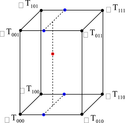
Figure 3. Schematic diagram of trilinear interpolation.

$\Delta {\mathbf{T}}_{ijk}\left(i,j,k\in \left\{0,1\right\}\right)$ represents the values of the eight corner points used for linear interpolation. The red dot represents the interpolation point, and the plane it appears on indicates an interpolation sequence. The interpolation sequence does not affect the interpolation results.

In the calculation, the interpolation weighting matrices, i.e., ${\mathbf{Q}}_1$, ${\mathbf{Q}}_2$, $\mathbf{J}$, and $\mathbf{P}$, are all sparse matrices. After removing the zero-valued elements in the above matrices, the storage space can be significantly reduced. Among them, the dimension of matrix ${\mathbf{Q}}_1$ can change from $N_{\Delta Tc}\times N_{\Delta Ts}$ to $N_{\Delta Tc}\times N_{ns\times ns}$. $ns\times ns$ represents the number of observation points used for local continuation. During calculation, the value of p ranging from 32 to 128 can meet the calculation accuracy requirements; the dimension of the matrix ${\mathbf{Q}}_2$ can change from $N_{\Delta Tc}\times N_{\Delta Ts}$ to $8\times N_{\Delta Ts}$; the dimension of the matrix $\mathbf{J}$ can change from $8N_{\Delta Tc}\times N_{\Delta Ts}$ to $N_{\Delta Tc}\times N_{ns\times ns}$; the dimension of the matrix $\mathbf{P}$ can change from $N_{\Delta Tc}\times 8N_{\Delta Tc}$ to $N_{\Delta Tc}\times 8$. By reducing the dimension of the above matrices, the fast calculation can be completed with only a small amount of computation cost.

2.3 Fast algorithm for magnetic anomaly of undulating surface

Based on the magnetic forward model in Equations 2, 3, the Tikhonov (Tikhonov and Arsenin, 1977) regularization objective function, ${\rho }_{\phi }\left(\alpha \right)$, was constructed as follows:

${\rho }_{\phi }\left(\alpha \right)=\left\{{‖\mathbf{D}\left(\mathbf{\Delta }{\mathbf{T}}_c-\mathbf{Q}{\mathbf{V}}_s{\mathbf{M}}_{\mathbf{\phi }}\right)‖}_2^2+\alpha {‖\mathbf{W}\left({\mathbf{M}}_{\mathbf{\phi }}-{\mathbf{M}}_{\mathbf{\phi }0}\right)‖}_2^2\right\},(6)$

where ${\mathbf{M}}_{\mathbf{\phi }}$ is the expected susceptibility model, $\alpha$ is the regularization factor; ${‖\mathbf{D}\left(\mathbf{\Delta }{\mathbf{T}}_c-\mathbf{Q}{\mathbf{V}}_s{\mathbf{M}}_{\mathbf{\phi }}\right)‖}_2^2$ is the fitting difference objective function of the magnetic field, ${‖\mathbf{W}\left({\mathbf{M}}_{\mathbf{\phi }}-{\mathbf{M}}_{\mathbf{\phi }0}\right)‖}_2^2$ is the Tikhonov regularization objective function, $\mathbf{D}$ is the diagonal data covariance matrix, where the elements on its diagonal are the estimated data noise variance, ${\mathbf{M}}_{\mathbf{\phi }0}$ is the reference model, $\mathbf{W}$ is the model weighting matrix, and $\mathbf{\Delta }{\mathbf{T}}_c$ represents the measured magnetic field value.

The inverse calculation determines the minimum solution value of the objective function (Equation 6). The gradient at the minimum value of the objective function is 0. The expression for the fixed-point iteration equation of model ${\mathbf{M}}_{\mathbf{\phi }}$ in the model space can be obtained as follows:

${\mathbf{M}}_{\mathbf{\phi }}={\mathbf{M}}_{\mathbf{\phi }0}+{\left({\mathbf{V}}_s^T{\mathbf{Q}}^{\mathbf{T}}{\mathbf{D}}^{\mathbf{T}}\mathbf{\text{DQ}}{\mathbf{V}}_s+\alpha {\mathbf{W}}^{\mathbf{T}}\mathbf{W}\right)}^{-1}{\mathbf{V}}_s^T{\mathbf{Q}}^{\mathbf{T}}{\mathbf{D}}^{\mathbf{T}}\mathbf{D}\left(\mathbf{\Delta }{\mathbf{T}}_c-\mathbf{Q}{\mathbf{V}}_s{\mathbf{M}}_{\mathbf{\phi }0}\right).(7)$

In this study, the three-dimensional inversion result of the magnetic susceptibility was obtained by applying the conjugate gradient algorithm to solve Equation 7.

3 Theoretical model experiments

Theoretical model tests were conducted for computation and testing on a computer with a processor speed of 2.20 GHz and a memory of 64 GB. This was the mainstream computer configuration for notebook workstations.

3.1 Efficiency comparison of forward modeling calculation

To compare the computational efficiency of the algorithms, models of different scales were used for comparative tests. The size of the prisms used to subdivide the underground space was 2 × 2 × 2 m. The number of subdivide cells of the model ranged from 9,216 to 45, 278, 208 (Table 1), and the latter is 4,913 times greater than the former. The lowest point of the undulating surface was 3 m, the highest point was set at 11 m, the maximum height difference was 8 m, and the spacing between the horizontal observation surfaces was 2 m.

Table 1

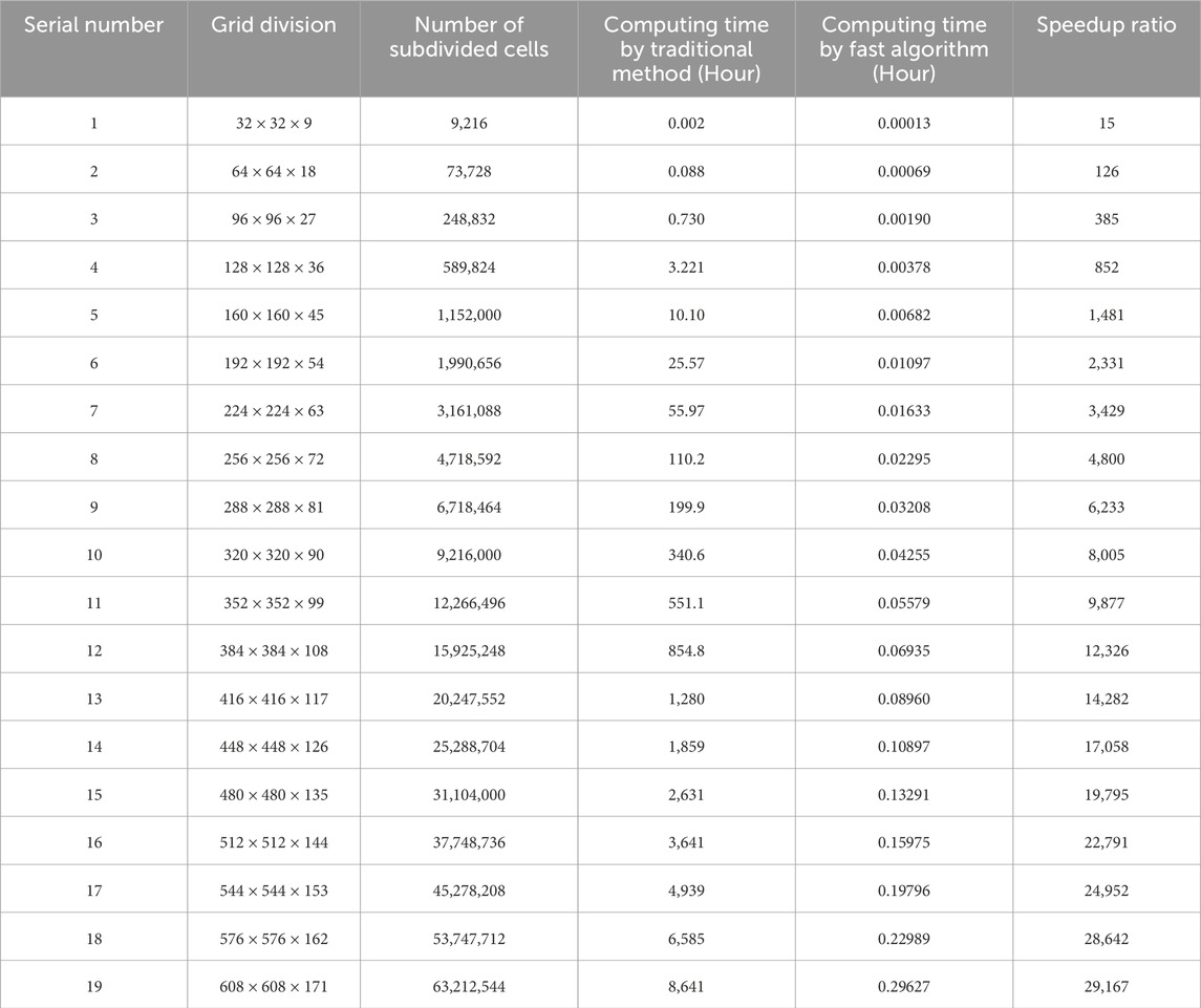
Table 1. The number of the subdivided cells and computational efficiency for different models.

For this series of models, forward calculations were performed using both traditional and fast algorithms. The traditional method uses the superposition principle to calculate the forward values of each observation point one by one and does not introduce any acceleration techniques. In the fast algorithm, the range of data points used for local continuation was set as 64 × 64 observation points. The number of computation points for the forward calculation was consistent with that of single-layer observation surface and they were randomly distributed with the horizontal center point of the observation grid as the center and a grid spacing as the radius (Figure 4). As the calculation time required for the forward calculation using the traditional algorithm exceeded the practical range, obtaining solutions through complete actual calculations was difficult. To effectively estimate the calculation time, the average time required for a single-point forward calculation was obtained by calculating a limited number of observation points and then multiplying by all of the observation points to obtain the estimated time for completing one forward calculation of this model.

Figure 4

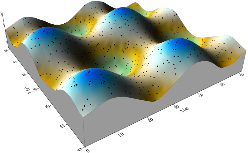
Figure 4. Schematic diagram of the distribution of any measuring points on the undulating surface.

The calculation results (Figure 5) show that the fast algorithm effectively improved the calculation efficiency. With an increase in the number of mesh divisions (Table 1), the acceleration effect of the fast algorithm became more notable. In other words, the speedup ratio increased and the maximum speedup ratio in the model example reached 29,167.

Figure 5

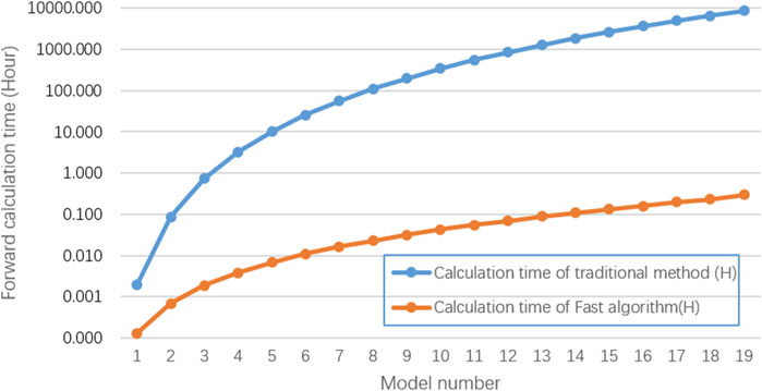
Figure 5. Comparison of computing time between the traditional and fast algorithms.

We note that the acceleration effect shown in the above calculations was not fixed. The speedup ratio was affected by several factors. One of the most important factors was the ratio between the degree of undulation of the terrain and the distance between the planes. If the elevation difference of the curved surface was greater and the plane spacing was smaller, more planes were required to cover the undulating curved surface, resulting in an increase in the number of calculations and a decrease in the speedup ratio.

3.2 Accuracy analysis of forward modeling computation

The purpose of this experiment was to compare the computational accuracy of three different interpolation methods: one is an interpolation method that only adopts local continuation; the second uses trilinear interpolation to correct all data based on the local continuation interpolation calculation; and the third uses trilinear interpolation to correct only the data at the boundary based on the local continuation interpolation calculation. We compared and analyzed the influence of different data ranges used for local continuation on the computational accuracy of these interpolation methods.

The model used in the test experiment consisted of four cuboidal magnetic bodies (Figure 6a). Table 2 lists the spatial positions and magnetic susceptibilities of the magnetic bodies. The side length of each model cube was 100 m and the elevation range of the underground space was −5,600 to 0 m. The magnetic field dip angle was 60° and the magnetic declination was –9°. The elevation range of the magnetic field undulation observation surface was 205.00 to 1,004.97 m (Figure 6b). The observation points were randomly on an undulating surface with average lateral distance of 100 m in each direction, totaling 39,204 observation points.

Figure 6

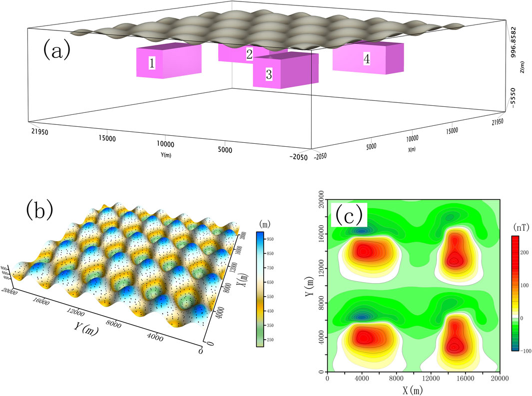
Figure 6. Schematic diagram of the model and forward modeling. (a) Schematic diagram of the model and undulating interface. (b) Schematic diagram of the distribution of measuring points on the undulating interface. (c) Calculated magnetic field produced by the model.

Table 2

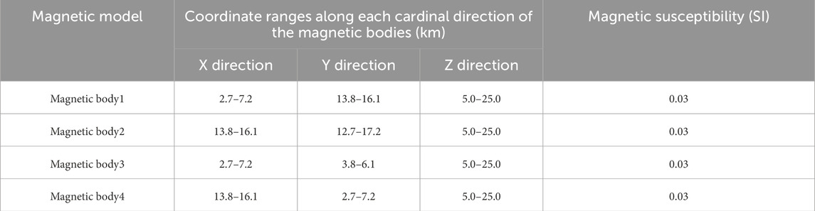
Table 2. Parameters of the magnetic body model.

The calculation accuracy of the forward field values of the model (Wu, 2018) was evaluated using the relative mean square error formula (Equation 8) as follows:

${\mathrm{E}}_{\text{err}}=\sqrt{\frac{{\displaystyle {\sum }_i}{\left(\Delta {\mathrm{T}}_i^c-\Delta {\mathrm{T}}_i\right)}^2}{{\displaystyle {\sum }_i}{\left(\Delta {\mathrm{T}}_i\right)}^2}}(8)$

where $\Delta {\mathrm{T}}_i$ represents the forward value of the magnetic field theory and $\Delta {\mathrm{T}}_i^c$ represents the forward value of the magnetic field based on the fast algorithm.

To compare the influence of different data ranges in the local continuation on the accuracy, the number of local continuation points selected in the experiment ranged from 32 × 32 to 158 × 158. The calculation results (Figure 7) show that the forward calculation accuracy of the three interpolation methods improved with an increase in ns. When only the interpolation method of local continuation was adopted, the relative error value first rapidly decreased from 2% to 0.6% (Local continuation interpolation) and converged. When the trilinear interpolation correction was used to correct all of the data, the relative error was basically stable at approximately 0.5% (Local continuation interpolation + Trilinear 1). When trilinear interpolation was used to correct only the boundary data, the relative error rapidly decreased from 1.6% and finally stabilized at approximately 0.2% (Local continuation interpolation + Trilinear 2).

Figure 7

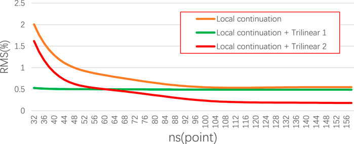
Figure 7. Comparison of the computational accuracy. ns (point) denotes the number of grid points in the x and y directions used for upward continuation calculations. The three types of tests are discussed in Figure 8 and in the text.

Based on the forward modeling error distribution map (Figure 8), when the value of ns was relatively small, the forward modeling errors of the three interpolation methods were mainly distributed in the regions with higher magnetic field anomaly values (Figures 8a–c). With an increase in ns, the forward modeling error using only the continuation interpolation method was effectively reduced in the middle area of the data (Figures 8a,d,g), but the error at the data edge did not significantly improve, whereas the forward modeling error when using trilinear interpolation to correct all of the data still remained large in the regions with higher magnetic field anomaly values; however, the error at the data edge was relatively small (Figures 8b,e,h). When using trilinear interpolation to correct only the boundary data for forward modeling errors, it combines the advantages of the above two methods, gradually reduces the forward modeling errors in both the central area and edge, and the error distribution is uniform, ultimately achieving the optimal forward modeling accuracy (Figures 8c,f,i).

Figure 8

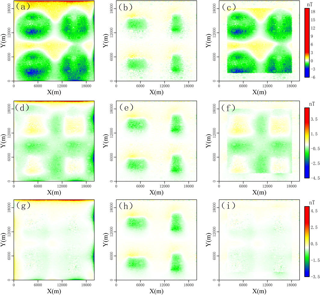
Figure 8. Comparison of the calculation errors. (a–c) are 32-point continuations. (d–f) are 64-point continuations. (g–i) are 128-point continuations. (a,d,g) are the forward modeling error diagrams calculated only by local continuation interpolation. (b,c,h) are the forward modeling error diagrams after correcting all data using trilinear interpolation based on local continuation. (c,f,i) are the forward modeling error diagrams after correcting only the data at the boundaries using trilinear interpolation based on local continuation.

The experiments show that the local interpolation correction method adopted in this study achieved relatively high calculation accuracy except at the edges.

3.3 The model study

In this experiment, a forward-field simulation of the measured magnetic field was performed using the model for the accuracy analysis, as described in Section 2.2. The subsurface space was divided into 200 × 200 × 56, totaling 2.24 million prisms. The prisms were set as cubes with side lengths of 100 m. The magnetic field inclination was 60.0° and the magnetic declination was −9.0°. The forward field of this model combination mainly consisted of four local anomalies with distorted isolines (Figure 6c).

The constraint methods for three-dimensional magnetic inversion mainly adopt depth weighting, focusing weighting, and physical property constraints. The physical property constraint sets the maximum magnetic susceptibility to 0.03 SI. The inversion result (Figure 9) was obtained through multiple calculation iterations. Compared with the theoretical model (Figure 6a), the spatial positions and shapes of the four magnetic anomalies had a good degree of coincidence.

Figure 9

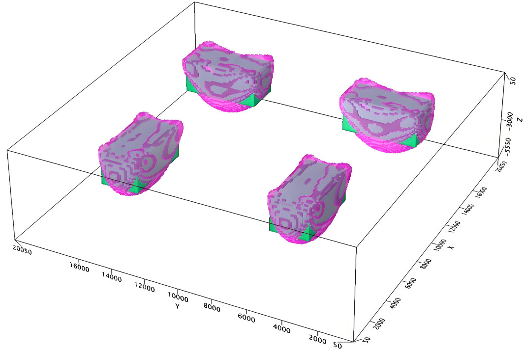
Figure 9. Schematic diagram of the three-dimensional inversion result of magnetic susceptibility.

The inversion results were further sliced in the horizontal (z = −1,000 m) and vertical directions (Figure 10). The slicing results show that the susceptibility distribution of the 3-D inversion results was mainly located within the spatial range of the theoretical model (blue-dashed box). The overall agreement with the theoretical model was high. This indicates that the forward and inversion algorithms for the undulating terrain proposed in this study have high inversion accuracy.

Figure 10

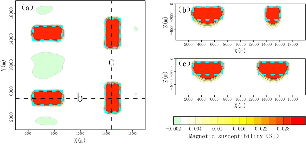
Figure 10. Slice maps of the three-dimensional inversion results of magnetic susceptibility (blue frame is the range of the theoretical model). (a) Horizontal slice of the model. (b,c) The vertical slice of the three-dimensional inversion model at the position of the dotted line in (a).

To simulate realistic data application (Figure 11a), a region with typical undulating characteristics was selected from the actual terrain and appropriately modified to be the undulating observation surface of the magnetic field, with an elevation range of 420.8–1,402.7 m above sea level (Figure 12a). A sloping plate-shaped magnetic body was set as the target body (Table 3). The body sloped northward with a dip angle of 45°. The dip angle of the magnetic field was 60.0° and the declination angle was −9.0°. The underground space was divided into 70 × 120 × 30, totaling 252,000 prisms, which were set as cubes with a side length of 100 m. The lateral average distance between the observation points on the curved surface was approximately 100 m.

Figure 11

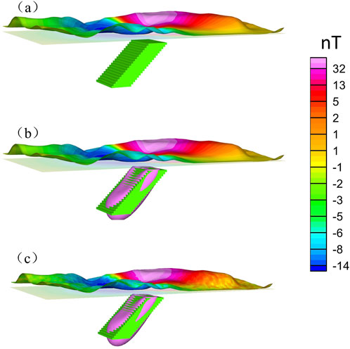
Figure 11. Schematic diagram of 3-D forward and inverse modeling of magnetic susceptibility. (a) 3-D inclined slab model and schematic diagram of the forward magnetic field. (b) 3-D inclined slab model, inverse result, and schematic diagram of the forward magnetic field. (c) 3-D inclined slab model, inverse result, and schematic diagram of the forward magnetic field with noise.

Figure 12

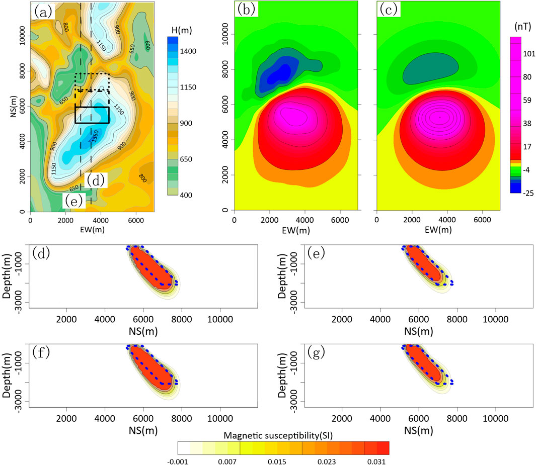
Figure 12. Comprehensive diagram of forward and inverse modeling. (a) Simulation of the actual undulating observation surface. (b) Forward magnetic field on the undulating observation surface. (c) Forward magnetic field on the horizontal plane at a height of 822.3 m (d,e) Vertical slices of the three-dimensional inversion model at the dotted line in (a). (f,g) Two vertical slices of the noise-contaminated magnetic three-dimensional inversion model at the dotted lines in (a).

Table 3

Table 3. Parameters of the second magnetic body model.

Based on the above model, forward magnetic field calculations were separately performed on curved surfaces and on a plane at the average elevation of the curved surface (822.3 m). The results show the forward modeling on the curved surface was significantly affected by the undulating observation surface compared with the smoother variations of the magnetic field on the plane (Figure 12c). Additionally, random noise (±2 nT) was introduced to evaluate the robustness of the method (Figure 11c).

The three-dimensional inversion adopted the same constraint strategy as in the previous model. The inversion result (Figures 11b,c) was obtained through multiple calculation iterations. The inversion results show a good agreement between the spatial geometry of the inverted magnetic anomalies and the theoretical model (Figure 11a), regardless whether the magnetic field contains noise or not. Furthermore, vertical slices of the inversion results were obtained (Figures 12d–g). The slice results show that the susceptibility distribution of the three-dimensional inversion result was mainly located within the spatial range of the theoretical model (blue-dashed box), regardless whether the noise data is contained. The overall coincidence with the theoretical model was high. This further indicates that the forward and inversion algorithms for undulating terrain proposed in this study also had high inversion accuracy in simulating actual situations.

4 Conclusion

This study proposed a method for improving the calculation efficiency for the three-dimensional forward modeling magnetic anomalies on undulating surfaces. This method has the following characteristics.

(1) The study proposed a new local interpolation combination method. Through two interpolation processes, it integrates the advantages of the upward continuation and trilinear interpolation methods. This method not only has practical physical significance, but also provides stable and reliable interpolation results, effectively ensuring the overall calculation accuracy of the algorithm.

(2) The traditional three-dimensional inversion method for magnetic anomalies on undulating surfaces often requires considerable computing resources during the calculation process. To address this issue, in this study, by fully utilizing the advantages of a fast forward calculation algorithm based on FFT for magnetic anomalies, the computing efficiency of the three-dimensional inversion of magnetic anomalies on undulating surfaces was significantly improved.

The algorithm proposed in this study has high potential for parallelism. The execution efficiency of this algorithm should improve with the introduction of parallel-computing technology. It should be noted that this method may not work well if there is significant remanent magnetization or the case that the magnetization is very high or anisotropy.

Data availability statement

The original contributions presented in the study are included in the article/Supplementary Material, further inquiries can be directed to the corresponding authors.

Author contributions

LJ: Formal Analysis, Writing – original draft, Visualization, Methodology. BD: Funding acquisition, Software, Writing – review and editing. LQ: Data curation, Methodology, Writing – original draft. MX: Writing – original draft, Project administration, Data curation. ZS: Writing – review and editing, Formal Analysis, Visualization. SS: Software, Writing – review and editing, Validation.

Funding

The author(s) declare that financial support was received for the research and/or publication of this article. This study is supported by the China Geological Survey Project (DD20230298; DD20240101901; DD202501028) and National Nonprofit Institute Research Grant (No. AS2024J10).

Acknowledgments

In particular, I would like to thank the reviewers and the editor for their valuable amendments and suggestions.

Conflict of interest

The authors declare that the research was conducted in the absence of any commercial or financial relationships that could be construed as a potential conflict of interest.

Generative AI statement

The author(s) declare that no Generative AI was used in the creation of this manuscript.

Publisher’s note

All claims expressed in this article are solely those of the authors and do not necessarily represent those of their affiliated organizations, or those of the publisher, the editors and the reviewers. Any product that may be evaluated in this article, or claim that may be made by its manufacturer, is not guaranteed or endorsed by the publisher.

Supplementary material

The Supplementary Material for this article can be found online at: https://www.frontiersin.org/articles/10.3389/feart.2025.1625616/full#supplementary-material

References

Bhattacharyya, B. K. (1964). Magnetic anomalies due to prism-shaped bodies with arbitrary polarization. Geophysics 29 (4), 517–531. doi:10.1190/1.1439386

CrossRef Full Text | Google Scholar

Bhattacharyya, B. K. (1980). A generalized multibody model for inversion of magnetic anomalies. Geophysics 45, 255–270. doi:10.1190/1.1441081

CrossRef Full Text | Google Scholar

Chen, L., and Liu, L. (2019). Fast and accurate forward modelling of gravity field using prismatic grids. Geophys. J. Int. 2019 (2), 1062–1071. doi:10.1093/gji/ggy480

CrossRef Full Text | Google Scholar

Dai, S., Zhu, D., Ying, Z., Kun, L., Chen, Q., Jiaxuan, L., et al. (2024). Three dimensional fast forward modeling of gravity anomalies under arbitrary undulating terrain. Chin. J. Geophys. (In Chinese) 67 (2), 768–780. doi:10.6038/Cjg2023q0605

CrossRef Full Text | Google Scholar

David, W. M., Mejer, H. T., and Arne, D. (2019). Inference of unexploded ordnance (UXO) by probabilistic inversion of magnetic data. Geophysical Journal International 1 (1). doi:10.1093/gji/ggz421

CrossRef Full Text | Google Scholar

Davis, K., and Li, Y. (2013). Efficient 3D inversion of magnetic data via octree-mesh discretization, space-filling curves, and wavelets. Geophysics 78 (5), J61–J73. doi:10.1190/GEO2012-0192.1

CrossRef Full Text | Google Scholar

Eppelbaum, L. V. (2011). Study of magnetic anomalies over archaeological targets in urban environments. Physics and Chemistry of the Earth 36 (16), 1318–1330. doi:10.1016/j.pce.2011.02.005

CrossRef Full Text | Google Scholar

Hogue, J. D., Renaut, R. A., and Vatankhah, S. (2019). A tutorial and open source software for the efficient evaluation of gravity and magnetic kernels. Computers and Geosciences 144, 104575. doi:10.1016/j.cageo.2020.104575

CrossRef Full Text | Google Scholar

Jing, L., Yao, C. L., Yang, Y. B., Xu, M. L., Zhang, G. Z., and Ji, R. Y. (2019). Optimization algorithm for rapid 3D gravity inversion. Applied Geophysics 16 (4), 507–518. doi:10.1007/s11770-019-0781-2

CrossRef Full Text | Google Scholar

Kirkby, A., and Duan, J. (2019). Crustal structure of the eastern arunta region, central Australia, from magnetotelluric, seismic, and magnetic data. Journal of Geophysical Research Solid Earth 124 (8), 9395–9414. doi:10.1029/2018JB016223

CrossRef Full Text | Google Scholar

Li, K., Long-Wei, C., Chen, Q., Dai, S. K., Zhang, Q. J., Zhao, D. D., et al. (2018). Fast 3D forward modeling of the magnetic field and gradient tensor on an undulated surface. Applied Geophysics 015 (003), 500–512. doi:10.1007/s11770-018-0690-9

CrossRef Full Text | Google Scholar

Li, Y., and Oldenburg, D. W. (2010). Fast inversion of large-scale magnetic data using wavelet transforms and a logarithmic barrier method. Geophysical Journal of the Royal Astronomical Society 152 (2), 251–265. doi:10.1046/j.1365-246X.2003.01766.x

CrossRef Full Text | Google Scholar

Li, Y., and Sun, J. (2016). 3D magnetization inversion using fuzzy c-means clustering with application to geology differentiation. Geophysics 81 (5), J61–J78. doi:10.1190/geo2015-0636.1

CrossRef Full Text | Google Scholar

Li, Y. G., and Oldenburg, D. W. (1996). 3-D inversion of magnetic data. Geophysics 61 (2), 394–408. doi:10.1190/1.1443968

CrossRef Full Text | Google Scholar

Liu, S., Maurizio, F., Xiangyun, H., Jamaledin, B., Bangshun, W., Zhang, D., et al. (2018). Extracting induced and remanent magnetizations from magnetic data modeling. Journal of geophysical research. Solid earth 123 (11), 9290–9309. doi:10.1029/2017jb015364

CrossRef Full Text | Google Scholar

Pilkington, M. (1997). 3-D magnetic imaging using conjugate gradients. Seg Technical Program Expanded Abstracts 15 (1), 1415–1418. doi:10.1190/1.1826377

CrossRef Full Text | Google Scholar

Pilkington, M. (2008). 3D magnetic data-space inversion with sparseness constraints. Geophysics 74 (1), L7–L15. doi:10.1190/1.3026538

CrossRef Full Text | Google Scholar

Portniaguine, O., and Zhdanov, M. S. (2000). 3-D magnetic inversion with data compression and image focusing. Geophysics 67 (5), 1532–1541. doi:10.1190/1.1512749

CrossRef Full Text | Google Scholar

Prutkin, I., and Saleh, A. (2009). Gravity and magnetic data inversion for 3D topography of the moho discontinuity in the Northern Red Sea area, Egypt. Journal of Geodynamics 47 (5), 237–245. doi:10.1016/j.jog.2008.12.001

CrossRef Full Text | Google Scholar

Qiang, J., Zhang, W., Lu, K., Chen, L., Zhu, Y., Hu, S., et al. (2019). A fast forward algorithm for three-dimensional magnetic anomaly on undulating terrain. Journal of Applied Geophysics 166, 33–41. doi:10.1016/j.jappgeo.2019.04.009

CrossRef Full Text | Google Scholar

Rezaie, M., Moradzadeh, A., and Kalateh, A. N. (2017). Fast 3D inversion of gravity data using solution space priorconditioned lanczos bidiagonalization. Journal of Applied Geophysics 136, 42–50. doi:10.1016/j.jappgeo.2016.10.019

CrossRef Full Text | Google Scholar

Shengxian, L., Center, C., and Survey, C. G. (2018). A self-constrained 3D inversion and efficient solution of gravity data based on cross-correlation coefficient. Journal of Jilin University(Earth Science Edition). doi:10.13278/j.cnki.jjuese.20170167

CrossRef Full Text | Google Scholar

Tikhonov, A. N., and Arsenin, V. Y. (1977). Solutions of Ill-posed problems. Winston, New York.

Google Scholar

Wu, L. (2018). Efficient modelling of gravity effects due to topographic masses using the Gauss–FFT method. Geophysical Journal International 205 (1), 160–178. doi:10.1093/gji/ggw010

CrossRef Full Text | Google Scholar

Yuan, Y., Cui, Y. A., Chen, B., Zhao, G. D., Liu, J. X., Guo, R. W., et al. (2022). Fast and high accuracy 3D magnetic anomaly forward modeling based on BTTB matrix. Chin. J. Geophys. (in Chinese) 65 (3), 1107–1124. doi:10.6038/cjg2022P0126

CrossRef Full Text | Google Scholar

Zeng, H. L. (2005). Gravity fields and gravity exploration. Beijing: Geology Press.

Google Scholar

Zheng, X., Liu, J., Chen, B., Zhao, G., Chen, L., Guo, R., et al. (2019). A fast and accurate gravity forward method for undulating structure model with surface observation. Computing techniques for geophysical and geochemical exploration.

Google Scholar