A fluid identification method for buried hill reservoirs based on a BP neural network model using NMR

The geological structure of buried hill reservoirs is highly complex. This study aims to develop a new reservoir fluid identification method for buried hill reservoirs by integrating nuclear magnetic resonance (NMR) logging techniques with a backpropagation (BP) neural network model. NMR logging data were used as input features, including parameters such as T_2g (geometric mean of the transverse relaxation time), A (amplitude of the last peak in the T₂ spectrum), S₃/S₁, and S₂/S₁. A BP neural network model was constructed with a single hidden layer consisting of eight neurons. The ReLU activation function was employed to accelerate the learning process, and the Softmax function was selected as the output layer activation function to accommodate multi-class classification requirements. Results show that the BP neural network model achieves superior performance in terms of precision, recall, and F1-score across four fluid types: oil zones, oil-water bearing zones, oil-bearing water zones, and water zones, outperforming other similar models. In Well HZ26-6-1 located in the ancient buried hill area, the model’s predictions are largely consistent with the results from well testing. This study demonstrates that the BP neural network-based approach not only significantly enhances the accuracy of fluid identification in reservoirs but also provides a scientifically sound and effective solution for fluid discrimination under complex geological conditions. Notably, the model exhibits strong classification capability in distinguishing between oil-water bearing zones and oil-bearing water zones, which are typically difficult to differentiate.

1 Introduction

As an important type of hydrocarbon reservoir, ancient buried-hill reservoirs possess significant advantages in terms of resource abundance. These reservoirs typically develop within ancient geological structures and have undergone prolonged geological evolution, leading to the formation of unique storage spaces. They are primarily characterized by high-permeability features such as fractures and dissolution cavities. Their primary advantage lies in excellent reservoir properties. Although porosity and permeability vary significantly across different regions, well-developed fracture zones can significantly enhance fluid mobility, enabling efficient hydrocarbon recovery. Accurately identifying fluid types and their distribution within the reservoir can further improve oil and gas recovery efficiency. However, ancient buried-hill reservoirs primarily consist of metamorphic and volcanic rocks, which have highly variable physical properties, making fluid identification more challenging. Additionally, the reservoir space is primarily controlled by fractures, resulting in highly variable fluid storage and flow characteristics. These complexities pose challenges for traditional logging methods in accurately identifying reservoir fluids. To address this issue, this study proposes a reservoir fluid identification method that selects optimal NMR parameters and employs a BP neural network. This method aims to address the limitations of conventional techniques, offering a more precise and reliable solution for reservoir fluid identification. Currently, the latest global methods for fluid identification using nuclear magnetic resonance (NMR) include the relaxation-diffusion two-dimensional NMR technique, which extends the representation of hydrogen nucleus distribution in pore fluids from a one-dimensional single T2 relaxation variable to a two-dimensional space incorporating both transverse relaxation time and diffusion coefficient. This approach enables effective differentiation between various fluid types such as oil, gas, and water. Another emerging method leverages T2 spectral morphological parameters through a deep learning architecture known as the Transformer model. By analyzing these morphological features extracted from NMR logging data and constructing labeled sample datasets, this approach trains robust fluid identification models with high accuracy. Additionally, an integrated fluid identification method combines NMR with acoustic (sonic) logging technologies, utilizing specially designed sonic-sensitive parameters to distinguish different fluid types—for example, identifying gas zones versus water zones—thereby enhancing the reliability of fluid typing under complex reservoir conditions.

Extensive research has been conducted on reservoir fluid identification using NMR technology. Kozlowski et al. (2021) have developed an integrated petrophysical workflow for the characterization of fluids and identification of contacts using both continuous and stationary NMR measurements in a high-porosity sandstone formation offshore Norway. Morshedy and Hossein (2018) have developed a three-dimensional modeling approach for reservoir fluid typing by integrating NMR data with thermophysical parameters. Li et al. (2024) have proposed a joint inversion technique that integrates multi-wait time and multi-echo time NMR logging data for improved fluid identification in reservoir characterization. Yang et al. (2023) developed a method for reconstructing LWD-NMR T₂ water spectra and performing fluid recognition by incorporating constraints from microscopic pore structures. However, existing reservoir fluid identification methods have limitations, including sensitivity to mineral composition and difficulty in distinguishing bound water from freely flowing oil-water mixtures (Archie, 1952). To overcome these challenges, this study proposes a backpropagation neural network model based on NMR data for fluid identification.

Compared to conventional logging data, NMR logging is unaffected by lithology, enables real-time monitoring, and delivers more accurate and detailed reservoir fluid parameters. This makes it particularly suitable for complex geological conditions or reservoirs that are challenging to evaluate using traditional methods. Lin et al. used clay mineral analysis, scanning electron microscopy and nuclear magnetic resonance (NMR) techniques to reveal the pore types and fluid states of the Upper Cretaceous oil shale (Lin et al., 2021). Although there have been no new studies on the interpretation of nuclear magnetic resonance in the petroleum industry in recent years, the application of nuclear magnetic resonance and deep learning technologies in other industries is relatively mature. For example, Jungeun et al. used liquid nuclear magnetic resonance (NMR) technology to discover that the decrease in the fluidity of the head group molecules of surfactants and the change in the octadecane overcooling degree during the thermal cycling process are the key factors leading to the instability of emulsions (Park et al., 2024). Asma et al. provided new insights into the mechanism of metal toxicity by combining proton nuclear magnetic resonance (1H NMR) and high-resolution mass spectrometry (HRMS) in a non-targeted metabolomics approach (Farjallah et al., 2024).

The BP neural network model, widely used in machine learning, offers several advantages for reservoir fluid identification, particularly in managing complex nonlinear relationships. First, the model’s multilayer architecture and nonlinear activation functions enable it to adapt to complex geological conditions, effectively capturing intricate patterns and enhancing prediction accuracy. Second, its strong self-learning capability allows it to automatically establish mapping relationships between input features and output labels from large training datasets, eliminating the need for manually designed algorithms or case-specific rules. Additionally, the BP neural network model offers high flexibility, enabling the integration of diverse data types and effectively leveraging multiple information sources to improve fluid identification accuracy. Therefore, based on relevant NMR logging data, this study develops a novel fluid identification method centered on the BP neural network model.

In this study, the BP neural network used for fluid identification differs from traditional machine learning methods in several key aspects. First, the input parameters selected are based on nuclear magnetic resonance (NMR) data, which are directly related to fluid properties, enabling the model to more accurately capture the differences between various fluid types during the learning process. Second, the method employs the ReLU activation function in the hidden layer and utilizes the Softmax function to address the multi-class classification problem. The ReLU activation function helps mitigate the vanishing gradient problem in deep networks, while Softmax ensures that the output probabilities sum to one, providing a probabilistic interpretation of each sample’s class membership. Finally, in terms of model architecture, a BP neural network with a single hidden layer containing eight neurons was constructed. The number of hidden neurons was determined through empirical formulas and experimentally validated to achieve optimal performance with eight nodes. This approach not only takes into account computational efficiency and the risk of overfitting, but also ensures that the model maintains strong generalization capability.

2 Geological backgrounds

The study focuses on the ancient buried-hill reservoir of the Huizhou Oilfield, situated in the eastern South China Sea within the Pearl River Mouth Basin, approximately 199 km southeast of Shenzhen, at an average water depth of about 113 m. The oilfield has proven geological reserves of 50 million cubic meters of oil equivalent, highlighting its significant production potential (Figure 1). The oilfield primarily contains reservoirs within the Paleogene and Neogene formations, with a particular emphasis on the ancient buried-hill reservoir in this study.

Figure 1

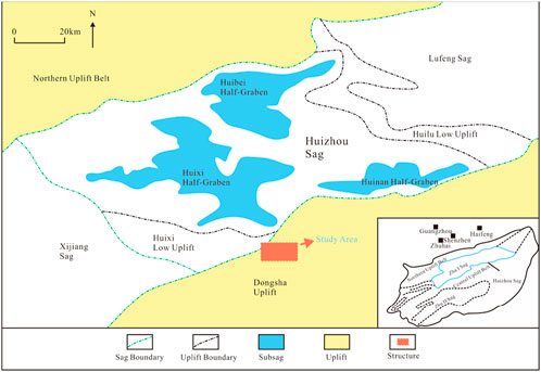
Figure 1. Location map of the study area.

The reservoirs in the study area are primarily controlled by fractures and exhibit strong heterogeneity (Figure 1). Hydrocarbon accumulation is influenced by multiple factors, including lithology and structural characteristics, leading to uneven reservoir distribution and complex fluid properties. Without accurate fluid identification prior to formation testing, potential high-yield zones may remain underutilized or improperly developed, resulting in increased production costs and possible resource wastage. Effective reservoir fluid identification can optimize the production process, enhance recovery efficiency and economic returns, and improve the understanding of fluid distribution within the reservoir. This, in turn, facilitates the selection of optimal extraction strategies and technologies.

3 Methods

3.1 Theoretical basis for reservoir classification and evaluation based on NMR logging data

For the study area, this paper uses the BP neural network algorithm to build a reservoir fluid property identification model, with the process identification principle (Figure 2). Neural network-based methods are developed by studying the structure of the human brain, creating units similar to biological neurons that are interconnected to approximate nonlinear relationships, thereby constructing nonlinear models. The flow diagram of the neural network method is shown below, consisting of three components: the input layer, hidden layer, and output layer. Different types of neural network methods, with varying propagation directions, have similar structures. Among them, the hidden layer is relatively more complex. In a BP neural network, errors are propagated backward, and this type of model can theoretically simulate various nonlinear mappings. However, different levels of complexity may lead to variations in training difficulty. Additionally, factors such as sample size and data distribution trends need to be considered.

Figure 2

Figure 2. Fluid identification principle diagram.

For the BP neural network, its computational process is as follows:

${\mathit{y}}_{\mathit{k}}={\displaystyle \sum _{\mathit{j}=\mathbf{1}}^{{\mathit{n}}_{\mathbf{2}}}}{\mathit{w}}_{\mathit{k}\mathit{i}}·\mathit{f}\left({\displaystyle \sum _{\mathit{i}=\mathbf{2}}^{{\mathit{n}}_{\mathbf{1}}}}{\mathit{w}}_{\mathit{i}\mathit{j}}{\mathit{x}}_{\mathit{i}}+{\mathit{b}}_{\mathit{i}}\right)$

In the above equation, x_i represents the input value, where x_i denotes the node number; w_i is the weight corresponding to the connected nodes, with the subscript indicating the number of connected nodes; b_i is the bias value; n₁ and n₂ correspond to the number of neurons in the input layer and output layer, respectively; $f\left({\displaystyle \sum _{i=2}^{n_1}}{W}_{ij}{X}_i+b_i\right)$ is the activation function; y_k on the left side of the equation represents the output value, where k is the node number.

$\mathit{E}=-\frac{\mathbf{1}}{\mathit{N}}\sum _{\mathit{i}}^{\mathit{N}}\left[{\mathit{y}}_{\mathit{i}}\mathit{log}\left({\mathit{y}}_{\mathit{k}}\right)+\left(\mathbf{1}-{\mathit{y}}_{\mathit{i}}\right)\mathit{log}\left(\mathbf{1}-{\mathit{y}}_{\mathit{k}}\right)\right]$

The equation above represents the error objective function E (cross-entropy loss), where y_i is the true value, y_k is the predicted value, and N is the number of samples. The success of the BP neural network lies in its ability to approximate complex nonlinear relationships by iteratively adjusting the weights. This adjustment process relies on an effective loss function and optimization strategy. Therefore, in this study, BP neural networks are employed for fluid identification, leading to enhanced fluid recognition performance.

3.2 Construction of the BP neural network input layer

Identifying reservoir fluids using neural networks involves establishing a mapping relationship between reservoir fluid properties and relevant parameters, making sample selection critical to the accuracy of the neural network model. In this study, NMR logging data is chosen as the primary dataset. The fundamental principle of NMR logging technology is based on the resonance behavior of hydrogen nuclei in formation fluids when exposed to an external magnetic field and radio frequency (RF) pulses (Krivdin, 2025; Eslami et al., 2013). When a strong magnetic field is applied, hydrogen nuclei in formation fluids align with the field according to their spin properties. Upon exposure to an RF pulse, these hydrogen nuclei deviate from their equilibrium alignment and enter an excited state. Once the RF pulse is removed, the nuclei gradually return to equilibrium, emitting signals during this relaxation process. By analyzing the decay of these signals, key fluid property parameters can be determined (Elsayed et al., 2022). Compared to conventional logging methods, NMR logging offers a more accurate and detailed characterization of reservoir fluids by directly detecting hydrogen nuclei. In contrast, traditional logging techniques often rely on multiple datasets and complex transformations to indirectly infer similar information. Thus, NMR logging provides higher-quality data support and deeper geological insights for petroleum exploration. It primarily measures the transverse relaxation time of pore fluids in the rock, which comprises bulk relaxation time, surface relaxation time, and diffusion relaxation time. These components are related as follows:

$\frac{\mathbf{1}}{{\mathit{T}}_{\mathbf{2}}}=\frac{\mathbf{1}}{{\mathit{T}}_{\mathbf{2}\mathit{B}}}+\frac{\mathbf{1}}{{\mathit{T}}_{\mathbf{2}\mathit{S}}}+\frac{\mathbf{1}}{{\mathit{T}}_{\mathbf{2}\mathit{D}}}=\frac{\mathbf{1}}{{\mathit{T}}_{\mathbf{2}\mathit{B}}}+{\mathit{\rho }}_{\mathbf{2}}\frac{\mathit{S}}{\mathit{V}}+\frac{\mathit{D}{\left(\mathit{\gamma }\mathit{G}{\mathit{T}}_{\mathit{E}}\right)}^{\mathbf{2}}}{\mathbf{12}}$

The bulk relaxation time is an intrinsic property of fluids, governed by their physical characteristics and influenced by factors such as temperature and viscosity (James et al., 2023; Davydov, 2016). Surface relaxation occurs at the solid-liquid interface, specifically on the surface of rock grains, and is controlled by the surface relaxation rate and pore size (Hooper Thomas et al., 2025). In a gradient magnetic field, fluids exhibit distinct diffusion relaxation characteristics when subjected to longer echo spacing. Crude oil with varying water content and formation water in different occurrence states display unique NMR relaxation signatures. Therefore, in this study, NMR logging data is utilized as the sample dataset, serving as the foundation for constructing the input layer of the BP neural network.

Constructing the input layer is a critical step in developing the BP neural network model, particularly in the selection of relevant features. Features that exhibit strong correlation with the target variable are chosen as inputs, either through statistical techniques or domain expertise (Guerrero and Carlos, 2024). The input layer must satisfy the following requirements: First, the input variables should have a significant impact on the output and be readily accessible. Second, the correlation between the variables should be minimized (Adediwura et al., 2024).

In this study, to enhance the accuracy of reservoir fluid identification, several parameters reflecting fluid characteristics are proposed based on NMR analysis, including T₂g (the geometric mean of transverse relaxation times between 10 and 300 m on the T₂ spectrum), the percentage of three pore components, and the amplitude of the last peak in the T₂ spectrum (Jin et al., 2022; Lucas-Oliveira and Ferreira, 2020). These parameters reflect the characteristics of pore fluids. The percentage of the three pore components refers to the ratio of the amplitude of the T₂ spectrum for transverse relaxation times less than 10 m, between 10 and 100 m, and greater than 100 m, relative to the total amplitude of the T₂ spectrum. This represents the proportion of small pores, medium pores, and large pores. The amplitude of the last peak of the T₂ spectrum represents the longitudinal amplitude component corresponding to the final peak of the T₂ spectrum. It reflects the proportion of large pores in rocks exhibiting bimodal characteristics (Figure 3).

Figure 3

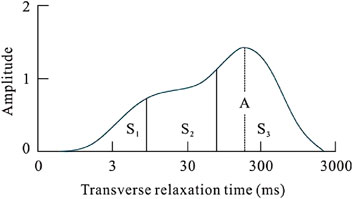
Figure 3. Illustration of T₂ spectrum in NMR logging.

In the study area of this paper, the proportions of various fluid types in the reservoir exhibit significant variation across different regions of the NMR T₂ spectrum. Typically, reservoirs with well-developed pore structures have higher oil content, characterized by a larger proportion of large pores and a smaller proportion of small pores. In contrast, rocks with poorly developed pore structures typically have lower oil content or may be devoid of oil, characterized by a smaller proportion of large pores and a larger proportion of small pores. The amplitude of the last peak in the T₂ spectrum also effectively reflects the reservoir’s internal structure, indicating the proportion of large pores in rocks exhibiting a bimodal characteristic (Blümich et al., 2004). Therefore, for this study, the selected input layer includes parameters such as T_2g (the geometric mean of the transverse relaxation time between 10 and 300 m on the T₂ spectrum), A (the amplitude of the last peak of the T₂ spectrum), S₃/S₁, and S₂/S₁.

For a specific machine learning algorithm, different features contribute differently to its performance. An excessive number of features can easily lead to the “curse of dimensionality,” increasing computational complexity and potentially degrading model performance. Selecting relevant features that significantly benefit the learning algorithm from the full feature set can greatly reduce computation time while improving both the model’s performance and interpretability.In this study, apart from the four aforementioned feature parameters, several conventional well logging parameters were also considered, including gamma ray (GR), compensated neutron log(CNL), bulk density (DEN), and spontaneous potential (SP). Due to the large number of feature types, a feature selection method was employed to reduce dimensionality and identify those features most sensitive to lithofacies classification. This not only helps improve model accuracy but also reduces computational cost and enhances the model’s generalization capability on new data. In this work, the decision tree method was selected as the feature selection approach. The decision tree-based feature selection method evaluates feature importance by calculating the Gini impurity, which serves as an indicator of each feature’s contribution to the classification task, thereby enabling effective feature reduction. Using decision tree-based feature selection, the importance scores of all well logging curve features were obtained, as summarized in Table 1. Based on these scores, four features with relatively high importance—T_2g, A, S₃/S₁, and S₂/S₁—were selected, indicating their high sensitivity to fluid typing. Six features with lower importance scores—namely GR, CNL, DEN, and SP—were excluded from further analysis (Table 1).

Table 1

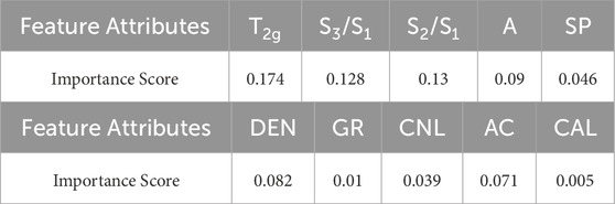
Table 1. Feature importance scores from decision tree-based feature selection.

The variations in NMR parameters after the inclusion of different fluids in the study area’s reservoirs are illustrated in the intersection diagrams:T_2g-S₂/S₁ intersection diagram (Figure 4), A-S₃/S₁ intersection diagram (Figure 5).

Figure 4

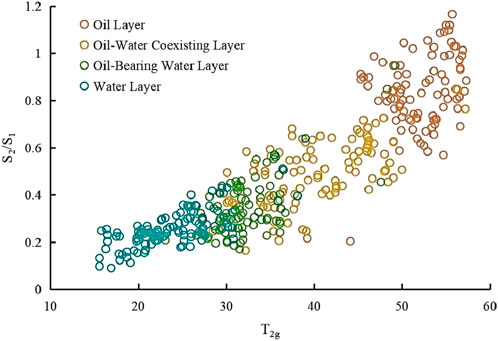
Figure 4. T_2g-S₂/S₁ intersection diagram.

Figure 5

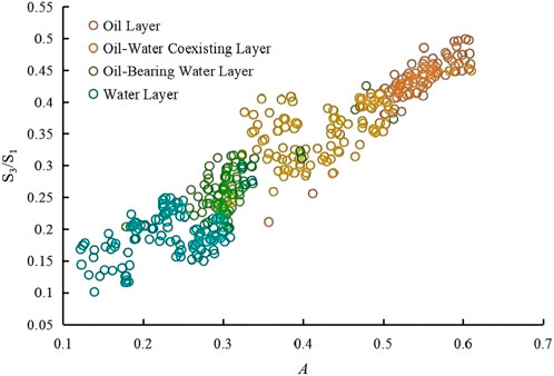
Figure 5. A-S₃/S1 intersection diagram.

As T_2g and A increase, there is a corresponding increase in oil content.As S₃/S₁ and S₂/S₁ increase, oil content also rises. These variations can be used for reservoir fluid identification, and by comparing these parameters, the reservoir evaluation process can be further optimized. However, relying solely on parameter evaluation still poses several challenges. As shown in the figures, the fluid parameter boundaries are quite vague and difficult to define. In the T_2g-S₂/S₁ diagram, it is evident that the data for oil-water coexisting layers and oil-bearing water Layers overlap significantly, making it challenging to distinguish between them. Similarly, in the A-S₃/S₁ intersection diagram, the boundaries between water layers and oil-bearing water layer, as well as between oil layers and oil-water coexisting layers, are unclear. Given these challenges, the BP neural network, known for its strong nonlinear mapping ability and adaptability, is employed in this study to tackle the fluid identification problem. The input layer consists of the following parameters: T_2g, A, S₂/S₁ and S₃/S₁.

To verify the feasibility and importance of the aforementioned parameters as input features and to evaluate their sensitivity, a univariate sensitivity analysis was performed on the input parameters. The main objective of this analysis is to assess the impact of each individual input feature on the model output, providing a basis for feature selection and optimization. By observing how changes in each input feature affect the model’s predictions, it is possible to identify which features are most influential in determining the output. The procedure involves systematically varying each input feature while keeping others constant, and quantifying its effect on the output of the BP neural network. The results of the univariate sensitivity analysis are presented in the figures.

The overall trend of the T_2g sensitivity analysis shows that as the perturbation value increases (Figure 6), the change in model output exhibits a decreasing tendency. Within the negative perturbation range (e.g., from −0.5 to −0.3), the model output demonstrates significant variation, whereas under positive perturbations (e.g., from 0 to 0.5), the changes in output are relatively small. The relationship is generally nonlinear, although it can be approximated as linear within certain intervals, such as from −0.5 to −0.3. In the negative perturbation range, the feature T_2g has a substantial impact on the model output, while its influence is weaker under positive perturbations.

Figure 6

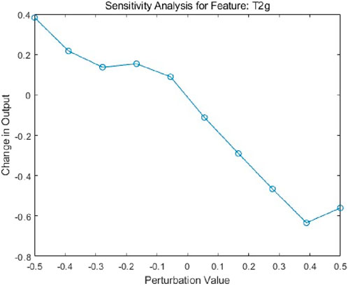
Figure 6. Sensitivity analysis for feature: T_2g.

The overall trend of the sensitivity analysis for feature A shows that as the perturbation value increases (Figure 7), the change in model output exhibits a decreasing pattern. Within the negative perturbation range (e.g., from −0.5 to −0.3), the model output undergoes significant changes, whereas under positive perturbations (e.g., from 0 to 0.5), the variations in output are relatively minor. Although the overall relationship is nonlinear, it can be approximated as linear within certain intervals, such as from −0.5 to −0.3. In the negative perturbation range, feature A has a considerable influence on the model output, while its impact is less pronounced under positive perturbations.

Figure 7

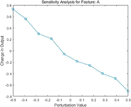
Figure 7. Sensitivity analysis for feature: A.

The overall trend of the sensitivity analysis for S₃/S₁ shows that as the perturbation value increases (Figure 8), the change in model output exhibits a fluctuating pattern. Within the negative perturbation range (e.g., from −0.5 to −0.3), the model output undergoes significant variation, whereas under positive perturbations (e.g., from 0 to 0.5), the changes in output are relatively minor. The relationship is predominantly nonlinear, although it can be approximated as linear within certain intervals, such as from −0.5 to −0.3. In the negative perturbation range, feature B has a substantial influence on the model output, while its impact is weaker under positive perturbations.

Figure 8

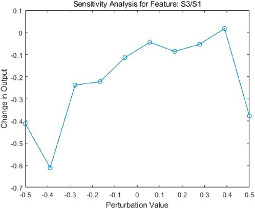
Figure 8. Sensitivity analysis for feature: S₃/S₁.

The overall trend of the sensitivity analysis for S₂/S₁ shows that as the perturbation value increases, the change in model output exhibits a decreasing pattern (Figure 9). Within the negative perturbation range (e.g., from −0.5 to −0.3), the model output undergoes significant variation, whereas under positive perturbations (e.g., from 0 to 0.5), the changes in output are relatively minor. The relationship is predominantly nonlinear, although it can be approximated as linear within certain intervals, such as from −0.5 to −0.3. In the negative perturbation range, the feature T2g has a substantial influence on the model output, while its impact is weaker under positive perturbations.

Figure 9

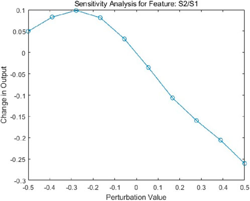
Figure 9. Sensitivity analysis for feature: S₂/S₁.

Based on the above analysis, it can be concluded that the features T_2g, A, S₂/S₁, and S₃/S₁ all have a significant impact on the model output. Considering their sensitivity and degree of linear relationship comprehensively, these features can be selected as input layers for the BP neural network.

3.3 Data normalization and construction of the BP neural network output layer

This study uses 400 core sample data from four wells in the research area, with a depth range of 3000m–4000m, as the training and testing dataset for the BP neural network model. Of these, 70% are allocated to the training set, 15% to the testing set, and 15% to the validation set. To ensure consistency in the measurement units of all input data and mitigate the effects of large disparities, the input parameters of the neural network are normalized to a range of 0–1 (Strahinja et al., 2024). Normalization plays a crucial role in the model’s training efficiency and performance, facilitating faster convergence, improving model stability, and enhancing its generalization capabilities. The input data for the BP neural network fluid identification are all processed through normalization:

$\mathit{X}=\frac{{\mathit{X}}_{\mathit{i}}-{\mathit{X}}_{\mathit{min}}}{{\mathit{X}}_{\mathit{max}}-{\mathit{X}}_{\mathit{min}}}$

In the equation: Xi represents the NMR parameter value; Xmin and Xmax denote the minimum and maximum values of the corresponding NMR parameter. The raw data for each NMR parameter is shown in Table 2, and the normalized extreme values are shown in Table 3.

Table 2

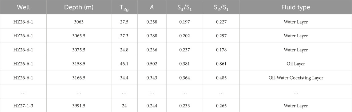
Table 2. Original fluid NMR logging dataset.

Table 3

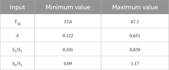
Table 3. Statistical table of normalized extremes for BP Neural Network model input parameters.

3.4 The determination of the number of hidden layers and nodes per layer

In BP neural networks, the number of hidden layers and the number of nodes per layer play a critical role in determining model performance. However, there is no fixed standard for selecting these parameters, as they depend heavily on the specific data characteristics, the problem’s complexity, and the desired performance of the model. For the model discussed in this study, a single hidden layer is sufficient. Adding more hidden layers would not only increase training time and computational costs but could also lead to overfitting issues (Chen and Wang, 2024). Therefore, a single hidden layer is used in this study.

The BP neural network utilized has a single hidden layer instead of more complex structures such as Convolutional Neural Networks (CNNs) or hybrid Long Short-Term Memory (LSTM) models. The primary reason for this choice is that increasing model complexity could lead to overfitting, where the model learns the details of the training set too thoroughly, including noise, resulting in poor performance on test sets or in practical applications. Moreover, compared to CNNs or LSTM models, the BP neural network’s internal mechanisms are more straightforward and intuitive, making it easier to trace back from the output to the influencing factors of the input. To verify the superiority of the single hidden layer in the BP neural network model in addressing this problem, comparisons were conducted with other learning models such as CNN and LSTM. Preliminary experiments were carried out for performance evaluation, and the results are summarized in Table 4. As shown in the table, the single hidden layer model significantly outperforms both CNN and LSTM (Table 4).

Table 4

Table 4. Model output results.

The number of hidden nodes is determined using the empirical formula:

${\mathit{N}}_{\mathit{h}}=\frac{{\mathit{N}}_{\mathit{s}}}{\left(\mathit{a}*\left({\mathit{N}}_{\mathit{i}}+{\mathit{N}}_{\mathit{o}}\right)\right)}$

The formula is as follows: In this, N_h represents the number of hidden layer nodes, N_i is the number of input layer nodes, No is the number of output layer nodes, N_s is the number of training samples, and a is a constant, ranging from 1 to 10.

In this study, N_s = 400, N_i = 4, and N_o = 4. The constant a is assigned different values, and the number of hidden layer nodes is initially determined to range between 4 and 10. By keeping other node parameters constant and analyzing the accuracy of the final results, a subset of data was selected for accuracy analysis. The accuracy analysis chart for different numbers of hidden layer nodes indicates that the highest accuracy is achieved when the number of hidden nodes reaches 8 (Figure 10). If the number of nodes exceeds 10, the risk of overfitting increases, and the computational cost rises. Therefore, in this study, the selected number of hidden nodes is 8.

Figure 10

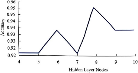
Figure 10. Accuracy analysis with different numbers of hidden layer nodes.

3.5 Selection of activation function

The activation function plays a critical role in BP neural networks, as it governs how the output of each neuron is transformed and directly affects the model’s learning ability and performance (Irani and Nasimi, 2011). For the application scenario described in this paper, which involves reservoir fluid identification based on NMR and a BP neural network model, the appropriate activation function has been selected.

For the output layer, the Softmax function is chosen as the activation function, as it is suitable for multi-class classification problems. The basic formula for the Softmax function is:

${\mathit{f}}_{\mathit{i}}\left(\mathit{x}\right)=\frac{{\mathit{e}}^{{\mathit{x}}_{\mathit{i}}}}{{\sum }_{\mathit{j}=\mathbf{1}}^{\mathit{n}}{\mathit{e}}^{{\mathit{x}}_{\mathit{j}}}}$

In the equation, i represents the class index, and n is the total number of classes. In reservoir fluid identification, the goal is typically to differentiate between mutually exclusive fluid types (such as oil, oil-water coexisting layers, oil-bearing water layers, and water). The Softmax function is ideal for this scenario because it ensures that the sum of all predicted probabilities equals 1. Additionally, the Softmax function converts the scores for each class into a probability distribution, providing a probability estimate for the sample’s membership in each category. The results processed by the BP neural network and Softmax function for a given output sample are shown in the following Table 5.

Table 5

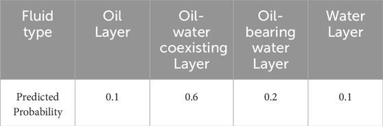
Table 5. Output distribution table.

From Table 5, it can be observed that the sample is most likely to belong to the oil-water coexisting layer (with the highest probability), followed by the oil-bearing water layer, oil layer, and water layer. Therefore, the output result is classified as the oil-water coexisting layer. As training progresses, the network’s weights are continuously adjusted through the backpropagation algorithm, causing the probability distribution output by the Softmax function to gradually become more focused. This process ultimately converges towards the correct classification. Ideally, for a given sample type, the Softmax output will assign the highest probability to that type, while the probabilities for other types will be lower.

For the hidden layer, the selected activation function is ReLU, and its basic calculation formula is as follows:

$\mathit{f}\left(\mathit{x}\right)=\mathit{max}\left(\mathbf{0},\mathit{x}\right)$

The ReLU function helps mitigate the vanishing gradient problem in deep networks. Given that reservoir fluid identification may involve complex geological conditions and nonlinear relationships, using ReLU can accelerate the model’s learning speed and enhance its expressive capacity. Additionally, ReLU’s computation is simpler and more direct, which helps speed up the training process. However, using ReLU as the activation function for the hidden layer may cause some neurons to output zero during the initial stages of training, leading to sparsity. Despite this, ReLU can still accelerate the training process and enhance the model’s ability to capture complex relationships. As training progresses, the model will gradually optimize the weights, improving its ability to identify different fluid types.

4 Results

4.1 BP neural network training and learning evaluation

The BP neural network training dataset comprises 400 samples, with 70% allocated for training, 15% for testing, and 15% for validation. The input layer consists of four parameters: T_2g, A, S₃/S₁, and S₂/S₁, while the output layer corresponds to four fluid types: oil layer, oil-water transition zone, oil-bearing water layer, and water layer. The network architecture includes four input neurons, 1 hidden layer with eight neurons, and four output neurons. A BP neural network model was developed using MATLAB, and its schematic diagram is presented (Figure 11).

Figure 11

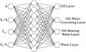
Figure 11. Schematic diagram of the fluid identification model structure.

The BP neural network training results are shown in the figure (Figure 12). In the figure, Class 1 represents the oil-bearing water layer, Class 2 represents the water layer, Class 3 represents the oil layer, and Class 4 represents the oil-water coexisting layer. The confusion matrix demonstrates that the BP neural network model exhibits strong classification performance across all datasets, with particularly high accuracy in the training and validation sets. The classification accuracy on the test set is also satisfactory, though some misclassifications are present. Overall, the model effectively distinguishes between oil-bearing water layers, water layers, oil layers, and oil-water coexisting layers, with no single category exhibiting significantly poor classification performance (Figure 12).

Figure 12

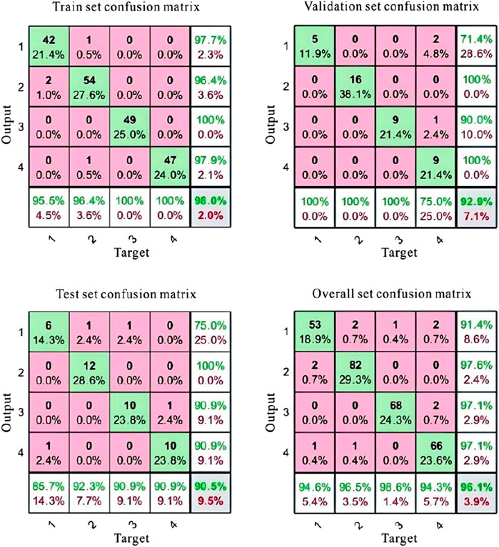
Figure 12. Confusion matrix.

Additionally, the ROC (Receiver operating characteristic) curve was plotted to evaluate the performance of the BP neural network model. The ROC curve is a graphical tool used to assess the effectiveness of classification models by illustrating the trade-off between the true positive rate and the false positive rate across different threshold settings. This curve provides valuable insight into the model’s discrimination ability and overall classification performance.

The ROC curve results for the BP neural network model are shown in the figure (Figure 13). The results indicate that the model demonstrates excellent classification performance across all datasets. The ROC curves for all fluid categories are close to the upper-left corner, suggesting that the model has strong distinguishing capability with high accuracy and a low false positive rate.

Figure 13

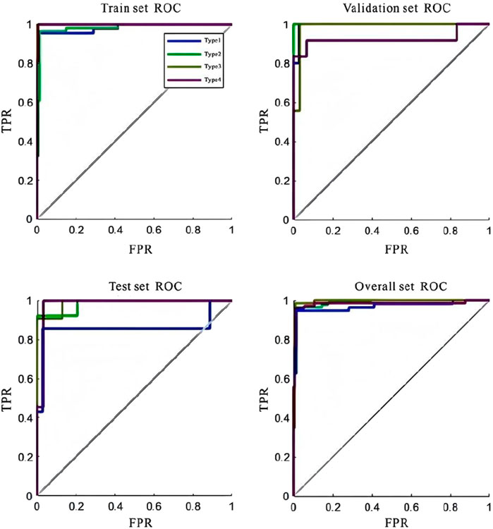
Figure 13. ROC curve of BPNN.

To further assess the performance of the BP neural network model, a fitness curve was generated. In machine learning, a fitness curve typically illustrates the evolution of the model’s performance metrics over time, such as during training epochs or iterations. This curve helps monitor the model’s convergence, identify potential overfitting or underfitting, determine the appropriate stopping criteria, and gain insights into the model’s learning rate.

The fitness curve is shown in the figure (Figure 14). From this curve, it can be observed that while the training error is very low in the later stages, the validation and test errors exhibit a slight increase, which may suggest a mild overfitting tendency. Overall, the model continues to perform well on the validation and test sets. Additionally, all error curves stabilize after approximately the fifth epoch, indicating that the model has essentially converged. This suggests that the model exhibits strong learning capability and generalization ability during training. The training, validation, and test errors decrease rapidly in the early stages and stabilize in the later epochs, reflecting consistent performance across the training, validation, and test datasets.

Figure 14

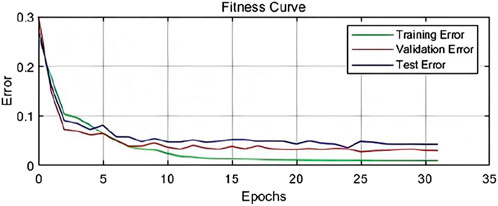
Figure 14. Fitness curve of BPNN.

Based on the results above, the BP neural network model was used to generate the BP network classification error chart and the network prediction result chart, as shown in the figures. The BP network classification error chart shows that the model performs excellently on most samples (Figure 15), with errors close to zero, although a few misclassifications can be observed in some samples (Figure 16). From the network prediction result chart, it is evident that the model performs excellently on most samples, with the predicted fluid types being highly consistent with the true fluid types. However, a few samples exhibit larger prediction errors, which may suggest potential issues or anomalies in these specific samples.

Figure 15

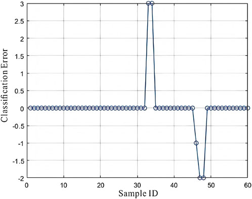
Figure 15. Network classification error chart.

Figure 16

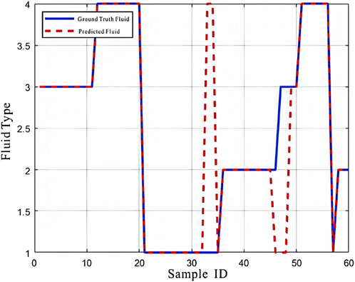
Figure 16. Network prediction result chart.

The selected prediction results presented in Table 6 show 11 matching cases, indicating the model’s effectiveness in reservoir fluid identification within the study area and its potential for practical application.

Table 6

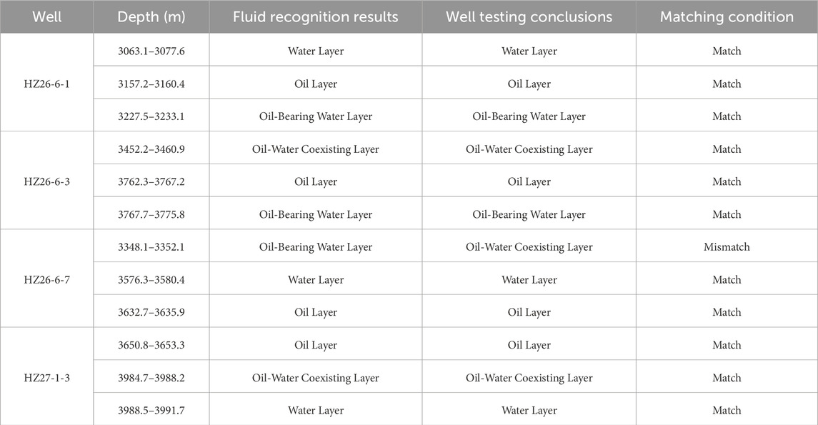
Table 6. Comparison of neural network identification results and well test results.

4.2 Validation of BP neural network model prediction results

To validate the prediction performance of the BP neural network model, other relevant classification models were selected to retrain the data and validate the model using test set data. The comparison models chosen include Decision Tree (DT), Support Vector Machine (SVM), and K-Nearest Neighbors (KNN). The DT model is capable of revealing the structured information within the data, extracting hidden knowledge rules, and automatically selecting the optimal boundary between classes based on the differences between data. The SVM model performs non-linear mapping, transforming the data from a lower-dimensional input space to a higher-dimensional feature space, allowing better identification, extraction, and classification in this higher-dimensional space. By constructing a new classification function in feature space based on certain criteria, SVM makes the data linearly separable. The KNN model classifies a sample by finding the nearest neighbors and assigning the sample to the majority class among these neighbors (Arafat et al., 2024; Sylwester, 2024; Goodarzi et al., 2025; Federica et al., 2025).

To validate the performance of the four models, the parameters used are precision, recall, and F1 score (Zhu et al., 2015; Maoucha et al., 2025; Wolpert, 1992; Kraipat et al., 2025). These three parameters all require the introduction of the basic concepts of true positives (TP), false positives (FP), true negatives (TN), and false negatives (FN) (Sun et al., 2025). TP refers to when the model correctly predicts an instance as positive, FP refers to when the model incorrectly predicts an instance as positive, TN refers to when the model correctly predicts an instance as negative, and FN refers to when the model incorrectly predicts an instance as negative (Kottayat et al., 2023; Lingampally Sai et al., 2023). The formula for precision is

$\mathit{P}\mathit{r}\mathit{e}\mathit{c}\mathit{i}\mathit{s}\mathit{i}\mathit{o}\mathit{n}=\frac{\mathit{T}\mathit{P}}{\mathit{T}\mathit{P}+\mathit{F}\mathit{P}}$

The formula for recall is:

$\mathit{R}\mathit{e}\mathit{c}\mathit{a}\mathit{l}\mathit{l}=\frac{\mathit{T}\mathit{P}}{\mathit{T}\mathit{P}+\mathit{F}\mathit{N}}$

This is example 1 of an equation:

$\mathit{F}\mathbf{1}=\frac{\mathbf{2}*\left(\mathit{P}\mathit{r}\mathit{e}\mathit{c}\mathit{i}\mathit{s}\mathit{i}\mathit{o}\mathit{n}*\mathit{R}\mathit{e}\mathit{c}\mathit{a}\mathit{l}\mathit{l}\right)}{\left(\mathit{P}\mathit{r}\mathit{e}\mathit{c}\mathit{i}\mathit{s}\mathit{i}\mathit{o}\mathit{n}+\mathit{R}\mathit{e}\mathit{c}\mathit{a}\mathit{l}\mathit{l}\right)}$

The training data was used to train the three alternative models, and then the performance of each model was evaluated using the test set data.

For the data of each fluid layer, as shown in the figures (Figures 17–20).

Figure 17

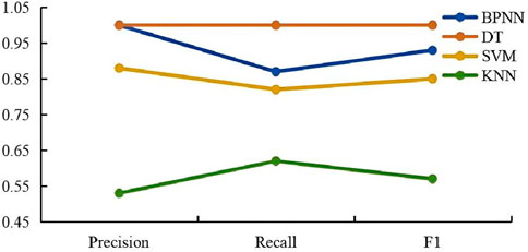
Figure 17. Oil layer parameter comparison chart.

Figure 18

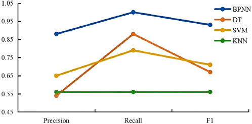
Figure 18. Oil-water coexisting layer parameter comparison chart.

Figure 19

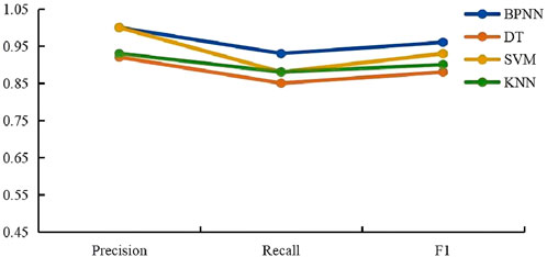
Figure 19. Water layer parameter comparison chart.

Figure 20

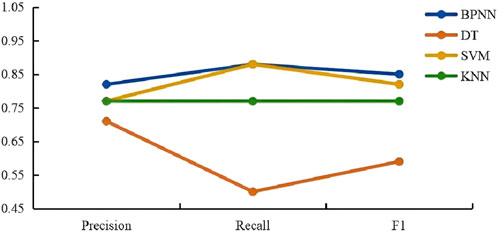
Figure 20. Oil-Bearing water layer parameter comparison chart.

A comprehensive analysis of the figures indicates that the BP neural network exhibits superior performance compared to other models in identifying different reservoir fluid types, including oil-water coexisting layers, oil layers, water layers, and oil-bearing water layers. The key reasons are as follows:

Precision: The BP neural network exhibits high precision across all fluid types, with exceptional performance in identifying oil-water coexisting layers and oil-bearing water layers, where its precision notably exceeds that of other models.

Recall: Although the recall of the BP neural network is slightly lower than that of the decision tree (DT) model for oil layers, it consistently maintains a high recall rate across most instances.

F1 Score: F1 Score: The F1 score, as the harmonic mean of precision and recall, reflects the balance between these two metrics. The BP neural network achieves high F1 scores across all fluid types, demonstrating its strong ability to maintain both precision and recall effectively.

Considering precision, recall, and F1 score collectively, the BP neural network shows the best overall performance across these datasets. It effectively captures complex data patterns and offers stable reservoir fluid identification. In contrast, other models show significant performance degradation, especially in oil-water-bearing and oil-water coexisting layers.

To further validate this conclusion, classification error charts and prediction result charts are shown in the figures (Figures 21, 22).

Figure 21

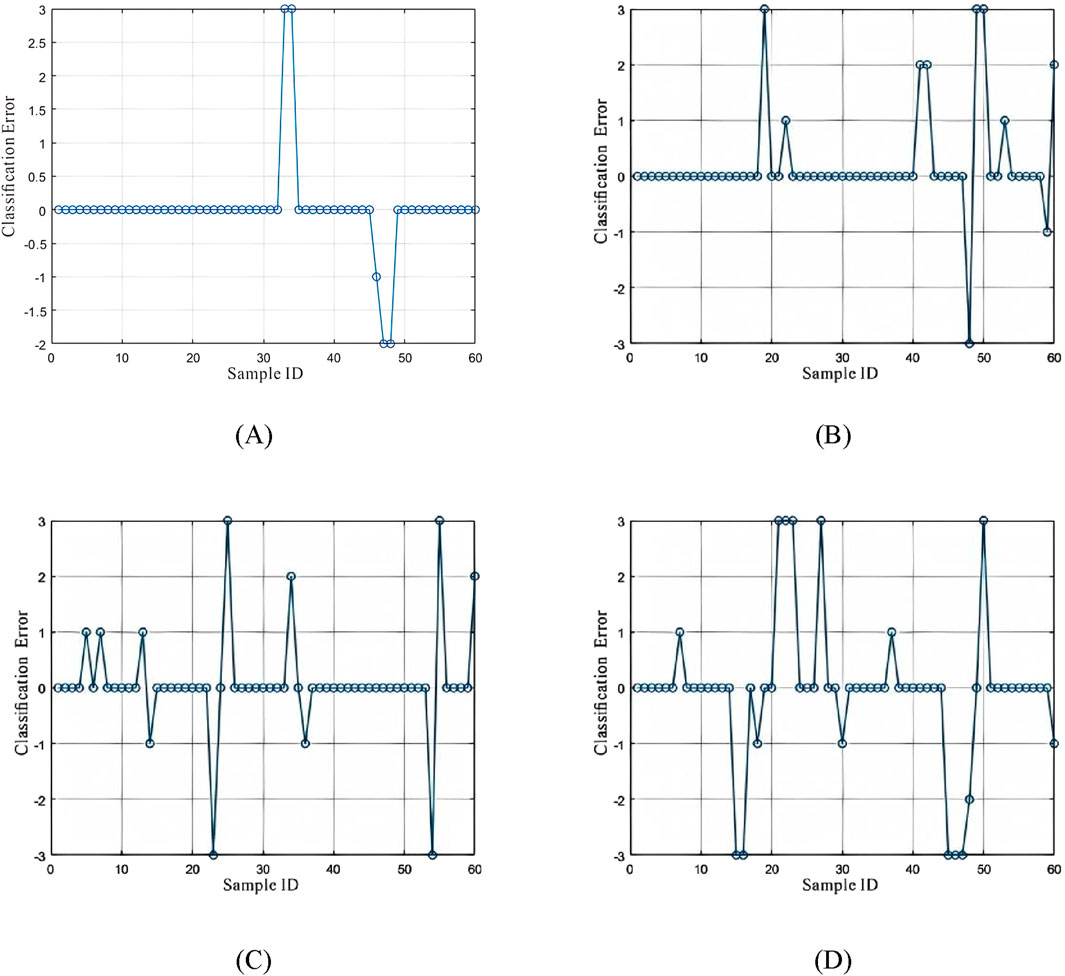
Figure 21. Classification error chart. (A) BP Neural Network classification error; (B) DT classification error; (C) SVM classification error; (D) KNN classification error.

Figure 22

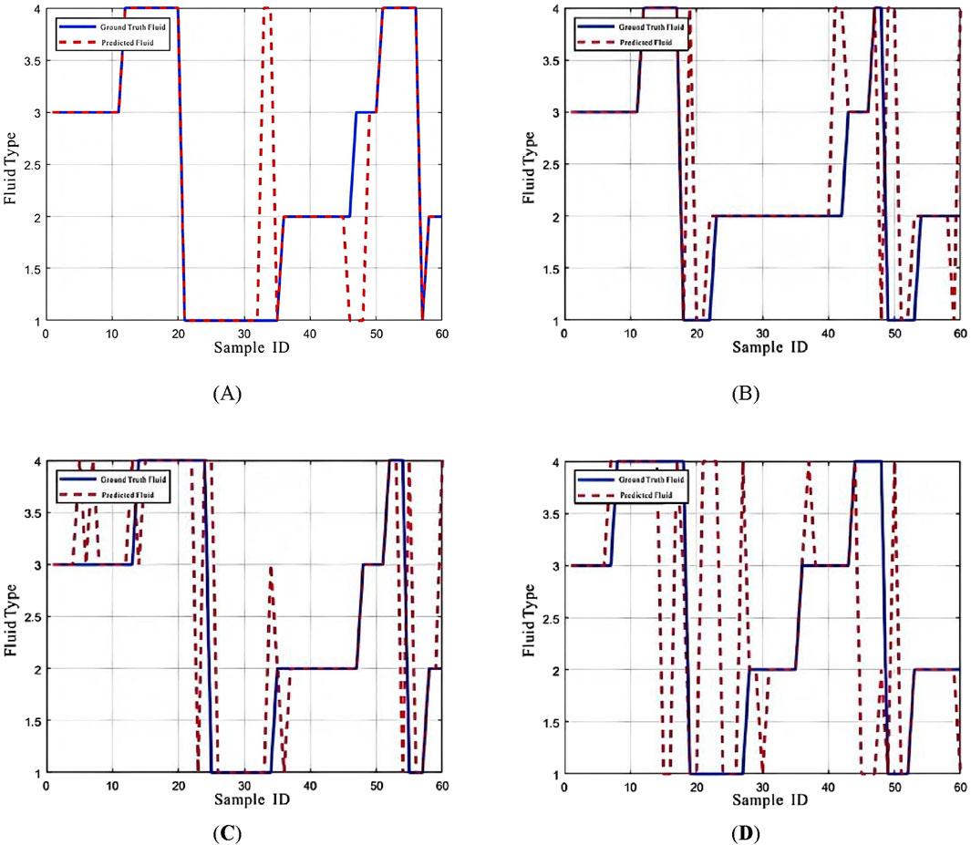
Figure 22. Prediction result chart. (A) BP Neural Network classification error; (B) DT classification error; (C) SVM classification error; (D) KNN classification error.

Through the classification error chart and prediction results, all four models exhibit strong performance in identifying reservoir fluids based on NMR logging data, achieving high prediction success rates. However, the KNN, DT, and SVM models have significantly higher classification errors than the BP neural network, with notably lower prediction accuracy. This demonstrates the BP neural network’s significant advantage in fluid identification, effectively overcoming the limitations of traditional fluid identification methods.

This model has been well validated within a single-porosity system; however, further validation is still required in a typical dual-porosity system. To this end, the model is validated separately within the matrix porosity system and the fracture porosity system. The results obtained are summarized in Table 7.

Table 7

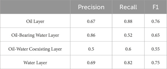
Table 7. Output results for dual-porosity systems.

The model performs poorly in the dual-porosity system, with significantly lower scores (Table 7). To address this issue, the outputs of the dual-porosity system were separated and trained individually. The results are presented in Tables 8, 9.

Table 8

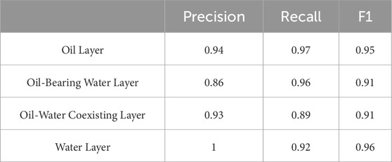
Table 8. Output results for matrix porosity system.

Table 9

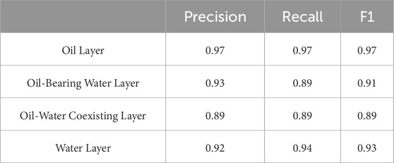
Table 9. Output results for fracture porosity system.

As shown in Tables 8, 9, the model achieves better performance after separate training for each pore system. If this model is to be applied in a typical dual-porosity system, it is necessary to first classify the system into its two constituent pore types, and then apply the model separately to each for validation (Tables 8, 9).

5 Discussion

Using the previously discussed models, the reservoir fluid properties of well HZ26-6-1 in the study area were analyzed. The depth interval from 3680 m to 3720 m was selected for prediction, and the results are presented in the figure (Figure 23).

Figure 23

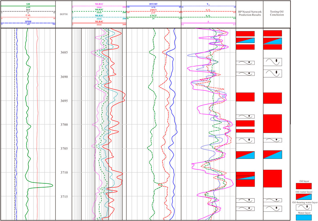
Figure 23. BP Neural Network-Based fluid identification for reservoir HZ26-6-1.

The reservoir fluid identification results show that the BP neural network model, developed using NMR data, provides predictions that are generally consistent with the oil testing results. Only a small portion of oil layers were misclassified as oil-water coexisting or oil-bearing water layers, demonstrating a high accuracy rate. This consistency between the BP neural network’s predictions and the actual oil testing results underscores the model’s effectiveness in overcoming the challenges of complex reservoir fluid identification.

6 Conclusion

This study integrates nuclear magnetic resonance (NMR) logging technology with a backpropagation (BP) neural network model to propose a new method for reservoir fluid identification, and validates its effectiveness.

(1) Innovatively selected NMR parameters as input feature variables: T2g, A (the amplitude of the last peak in the T2 spectrum), S3/S1, and S2/S1 were chosen as input features, significantly improving the accuracy of reservoir fluid identification.

(2) The BP neural network model was optimized: a BP neural network with a single hidden layer containing eight neurons was constructed. The ReLU activation function was employed to accelerate the learning process, and the Softmax function was used to handle the multi-class classification problem. The model outperformed other comparative models in terms of precision, recall, and F1-score across four fluid types: oil zones, oil-water bearing zones, oil-bearing water zones, and water zones.

(3) Through a case study on Well HZ26-6-1, the model’s predictions were found to be highly consistent with the results from well testing, demonstrating high accuracy. This indicates that the BP neural network not only effectively identifies reservoir fluid properties, but also provides solutions to challenges commonly encountered in traditional fluid identification methods.

Data availability statement

The original contributions presented in the study are included in the article/Supplementary Material, further inquiries can be directed to the corresponding author.

Author contributions

MW: Conceptualization, Data curation, Formal Analysis, Funding acquisition, Investigation, Methodology, Project administration, Resources, Software, Supervision, Validation, Visualization, Writing – original draft, Writing – review and editing. QZ: Conceptualization, Data curation, Formal Analysis, Funding acquisition, Investigation, Methodology, Project administration, Resources, Software, Supervision, Validation, Visualization, Writing – original draft, Writing – review and editing. LY: Conceptualization, Data curation, Formal Analysis, Funding acquisition, Investigation, Methodology, Project administration, Resources, Software, Supervision, Validation, Visualization, Writing – original draft, Writing – review and editing. HX: Conceptualization, Data curation, Formal Analysis, Funding acquisition, Investigation, Methodology, Project administration, Resources, Software, Supervision, Validation, Visualization, Writing – original draft, Writing – review and editing.

Funding

The author(s) declare that no financial support was received for the research and/or publication of this article.

Acknowledgments

A heartfelt thank you to every individual and institution that contributed to this research.

Conflict of interest

Authors MW, QZ, LY, and HX were employed by China Oilfield Services Limited Co. Ltd.

Generative AI statement

The author(s) declare that no Generative AI was used in the creation of this manuscript.

Publisher’s note

All claims expressed in this article are solely those of the authors and do not necessarily represent those of their affiliated organizations, or those of the publisher, the editors and the reviewers. Any product that may be evaluated in this article, or claim that may be made by its manufacturer, is not guaranteed or endorsed by the publisher.

Supplementary material

The Supplementary Material for this article can be found online at: https://www.frontiersin.org/articles/10.3389/feart.2025.1632339/full#supplementary-material

References

Adediwura, S. C., Neeshma, M., and Auf, D. G. J. S. (2024). Combining NMR and impedance spectroscopy in situ to study the dynamics of solid ion conductors. J. Mater. Chem. A 12, 15847–15857. doi:10.1039/d3ta06237f

CrossRef Full Text | Google Scholar

Arafat, M. Y., Hossain, M. J., and Alam, M. M. (2024). Machine learning scopes on microgrid predictive maintenance: potential frameworks, challenges, and prospects. Renew. and Sustain. Energy Rev., 190. doi:10.1016/j.rser.2023.114088

CrossRef Full Text | Google Scholar

Archie, G. E. (1952). Classification of carbonate reservoir rocks and petrophysical considerations. Bull. Am. Assoc. Petroleum Geol. 36, 278–298. doi:10.1306/3d9343f7-16b1-11d7-8645000102c1865d

CrossRef Full Text | Google Scholar

Blümich, B., Anferova, S., Pechnig, R., Pape, H., Arnold, J., and Clauser, C. (2004). Mobile NMR for porosity analysis of drill core sections. J. Geophys. Eng. 1, 177–180. doi:10.1088/1742-2132/1/3/001

CrossRef Full Text | Google Scholar

Chen, Q., and Wang, W. (2024). Prediction of shale gas horizontal well production using particle swarm optimisation-based BP neural network. Int. J. Oil Gas Coal Technol. 36, 449–460. doi:10.1504/ijogct.2024.142105

CrossRef Full Text | Google Scholar

Davydov, V. V. (2016). Some specific features of the NMR study of fluid flows. Opt. Spectrosc. 121, 18–24. doi:10.1134/s0030400x16070092

CrossRef Full Text | Google Scholar

Elsayed, M., Isah, A., Hiba, M., Hassan, A., Al-Garadi, K., Mahmoud, M., et al. (2022). A review on the applications of nuclear magnetic resonance (NMR) in the oil and gas industry: laboratory and field-scale measurements. J. Petroleum Explor. Prod. Technol. 12, 2747–2784. doi:10.1007/s13202-022-01476-3

CrossRef Full Text | Google Scholar

Eslami, M., Kadkhodaie-Ilkhchi, A., Sharghi, Y., and Golsanami, N. (2013). Construction of synthetic capillary pressure curves from the joint use of NMR log data and conventional well logs. J. Petroleum Sci. Eng. 111, 50–58. doi:10.1016/j.petrol.2013.10.010

CrossRef Full Text | Google Scholar

Farjallah, A., Roy, A., and Guéguen, C. (2024). NMR- and HRMS-Based untargeted metabolomic study of metal-stressed Euglena gracilis cells. Algal Res. 78, 103383. doi:10.1016/j.algal.2023.103383

CrossRef Full Text | Google Scholar

Federica, B., Bart, D., and Angelika, F. (2025). Machine learning approaches for the prediction of public EV charge point flexibility. Sustain. Energy Grids and Netwoks, 42. doi:10.1016/j.applthermaleng.2025.125527

CrossRef Full Text | Google Scholar

Goodarzi, R. M., Barzkar, A., Sabaghzadeh, M., ghanbari, M., and Fathollahzadeh Attar, N. (2025). Uncertainty analysis of machine learning methods to estimate snow water equivalent using meteorological and remote sensing data. Water Resour. Manag., 1–21. doi:10.1007/s11269-025-04164-z

CrossRef Full Text | Google Scholar

Guerrero, C., and Carlos, S. J. (2024). Assessment of hydrogen adsorption in high specific surface geomaterials using low-field NMR - Implications for storage and field characterization. Int. J. Hydrogen Energy 95, 417–426. doi:10.1016/j.ijhydene.2024.11.228

CrossRef Full Text | Google Scholar

Hooper Thomas, J. N., Oliveira-Silva Rodrigo, de, and Dimitrios, S. (2025). High-resolution in situ photo-irradiation MAS NMR: application to the UV-polymerization of n-butyl acrylate. J. Mater. Chem. A 13, 933–939. doi:10.1039/d4ta06729k

CrossRef Full Text | Google Scholar

Irani, R., and Nasimi, R. (2011). Application of artificial bee colony-based neural network in bottom hole pressure prediction in underbalanced drilling. J. Petroleum Sci. Eng. 78, 6–12. doi:10.1016/j.petrol.2011.05.006

CrossRef Full Text | Google Scholar

James, F., Myers, M., and Lori, H. (2023). NMR-mapped distributions of dielectric dispersion. Petrophysics 64, 421–437. doi:10.30632/pjv64n3-2023a7

CrossRef Full Text | Google Scholar

Jin, G. W., Wang, T. Y., and Liu, Z. H. (2022). Classification of glutenite reservoirs and productivity prediction method based on nuclear magnetic resonance (NMR) logging. Acta Pet. Sin. 43, 648–657. doi:10.7623/syxb202205006

CrossRef Full Text | Google Scholar

Kottayat, N., Dhruv, T., Kumar, Y. A., and Anish, S. (2023). Machine learning approach for optimization and performance prediction of triangular duct solar air heater: a comprehensive review. Sol. Energy 255, 396–415. doi:10.1016/j.solener.2023.02.022

CrossRef Full Text | Google Scholar

Kozlowski, M., Chakraborty, M., Jambunathan, V., Lowrey, P., Balliet, R., Engelman, B., et al. (2021). An integrated petrophysical workflow for fluid characterization and contacts identification using NMR continuous and stationary measurements in a high-porosity sandstone formation, offshore Norway. Petrophysics 62, 210–226. doi:10.30632/pjv62n2-2021a5

CrossRef Full Text | Google Scholar

Kraipat, C., Chaiwat, P., and Thossaporn, W. (2025). Machine learning-driven modeling of biomass pyrolysis product distribution through thermal parameter sensitivity. Renwable Energy, 248. doi:10.1016/j.renene.2025.123108

CrossRef Full Text | Google Scholar

Krivdin, L. B. (2025). Recent advances in 1D and 2D liquid-phase and solid-state NMR studies of biofuel. Renew. Energy, 243. doi:10.1016/j.renene.2025.122592

CrossRef Full Text | Google Scholar

Li, B., Tan, M. J., Zhang, H. T., Zhou, J., Changsheng, W., and Haopeng, G. (2024). Joint inversion method of nuclear magnetic resonance logging multiwait time and multiecho time activation data and fluid identification. Spe J. 29, 4054–4068. doi:10.2118/221452-pa

CrossRef Full Text | Google Scholar

Lin, T., Liu, X., Zhang, J., and Bai, Y. (2021). Characterization of multi-component and multi-phase fluids in the Upper Cretaceous oil shale from the songliao basin (NE China) using T1–T2 NMR correlation maps. Petroleum Sci. Technol. 39, 1060–1070. doi:10.1080/10916466.2021.1990318

CrossRef Full Text | Google Scholar

Lingampally Sai, V., Ram Madhab, B., and Nilabjendu, G. (2023). Machine learning approach for the prediction of mining-induced stress in underground mines to mitigate ground control disasters and accidents. Geomechanics Geophys. Geo-Energy Geo-Resources 9, 1–19. doi:10.1007/s40948-023-00701-5

CrossRef Full Text | Google Scholar

Lucas-Oliveira, E., and Ferreira, A. (2020). Sandstone surface relaxivity determined by NMR T2 distribution and digital rock simulation for permeability evaluation. J. Petroleum Sci. Eng., 193. doi:10.1016/j.petrol.2020.107400

CrossRef Full Text | Google Scholar

Maoucha, A., Berghout, T., and Djeffal, F. (2025). Machine learning-guided analysis of CIGS solar cell efficiency: deep learning classification and feature importance evaluation. Sol. Energy, 287. doi:10.1016/j.solener.2025.113251

CrossRef Full Text | Google Scholar

Morshedy, A., and Hossein, M. M. (2018). Fatehi. Three-dimensional modelling of reservoir fluid typing by applying nuclear magnetic resonance (NMR) and thermophysical parameters. Boll. Di Geofis. Ed. Appl. 59, 95–106. doi:10.4430/bgta0225

CrossRef Full Text | Google Scholar

Park, J., Ulrich, S., and Robert, J. (2024). MessingerCA1. molecular-level understanding of phase stability in phase-change nanoemulsions for thermal energy storage by NMR spectroscopy. Langmuir 41, 21814–21823. doi:10.1021/acs.langmuir.4c02997

CrossRef Full Text | Google Scholar

Strahinja, M., Aliya, M., and Alexey, C. (2024). Matrix decomposition methods for accurate water saturation prediction in Canadian oil-sands by LF-NMR T2 measurements. Geoenergy Sci. Eng., 233. doi:10.1016/j.geoen.2023.212438

CrossRef Full Text | Google Scholar

Sun, A., Tang, X., Liao, H., and Gong, J. (2025). Predicting ignitability classification of thermally thick solids using hybrid GA-BPNN and PSO-BPNN algorithms. Fuel 381, 133474. doi:10.1016/j.fuel.2024.133474

CrossRef Full Text | Google Scholar

Sylwester, B. (2024). Machine learning in cartel screening-the case of parallel pricing in a fuel wholesale market. Energies 17, 4184. doi:10.3390/en17164184

CrossRef Full Text | Google Scholar

Wolpert, D. H. (1992). Stacked generalization. Neural Netw. 5 (5), 241–259. doi:10.1016/s0893-6080(05)80023-1

CrossRef Full Text | Google Scholar

Yang, W. W., Zhang, C., and Shi, X. L. (2023). Reconstruction of LWD-NMR T2 water spectrum and fluid recognition based on microscopic pore structure constraints. Geoenergy Sci. Eng., 221. doi:10.1016/j.geoen.2022.211386

CrossRef Full Text | Google Scholar

Zhu, P., Lin, C., and Wu, P. (2015). Logging quantitative identification of diagenetic facies by using principal component analysis: a case of Es3x1 in Zhuang 62-66 area, Wu Hao-zhuang oilfeild. Prog. Geophys. 30, 2360–2365. doi:10.6038/pg20150551

CrossRef Full Text | Google Scholar