Improving Learning: Using a Learning Progression to Coordinate Instruction and Assessment

Introduction

In this paper, we illustrate the use of an organized learning model, specifically, a learning progression, to support instructionally useful assessment. Learning progressions guide instructional plans for nurturing students’ long-term development of disciplinary knowledge and dispositions (National Research Council, 2006). Establishing a learning progression is an epistemic enterprise (Knorr Cetina, 1999) in which students are positioned to participate in the generation and revision of forms of knowledge valued by a discipline. For that, we need both an instructional design and an assessment design, and the two needs to be tightly co-ordinated. In particular, the assessments inform crucial aspects of the progression: (a) they provide formative information for the development and refinement of the learning progression, and (b) they provide formative and summative information for teachers using the learning progression to iteratively refine instruction in response to evidence about student learning.

The idea of a learning progression is related to curriculum and instructional concepts that have been apparent in the educational literature for many years, and it is closely tied a learning trajectory as commonly used in mathematics education (Simon, 1995). One definition that has become prominent is the following:

Learning progressions are descriptions of the successively more sophisticated ways of thinking about an important domain of knowledge and practice that can follow one another as children learn about and investigate a topic over a broad span of time. They are crucially dependent on instructional practices if they are to occur (Center for Continuous Instructional Improvement (CCII), 2009).

This description is broadly encompassing, but, at the same time, the description signals something more than an ordered set of ideas, curriculum pieces, or instructional events: Learning progressions should characterize benchmarks of conceptual change and in tandem, conceptual pivots—conceptual tools and conjectures about mechanisms of learning that support the kinds of changes in knowing envisioned in the progression. Benchmarks of conceptual change are models of modal forms of student thinking and like other models, must be judged on their utility. They are ideally represented at a “mid-level” of description that captures critical qualities of students’ ways of thinking without being either so broad as to provide very little guidance for instruction and assessment, or so overwhelmingly fine-grained as to impede ready use. Similarly, conceptual pivots are ways of thinking and doing that tend to catalyze conceptual growth, and as such, are situated within a theoretically compelling framing of potential mechanisms of learning.

Further entailments of a learning progression include commitments about alignment of discipline, learning, instruction, and assessment. In our view, these include:

(a) an epistemic view of a discipline that describes how concepts are generated and warranted;

(b) representations of learning structured as descriptions of forms of student knowledge, including concepts and practices, and consequential transitions among these forms, as informed by the epistemic analysis;

(c) help for teachers to identify classes of student performances as representing particular forms of student knowledge around which teachers can craft instructional responses, and

(d) assessments and reports designed to help reveal students’ ways of thinking, and to organize evidence of such thinking in ways that help teachers flexibly adapt instruction.

Thus, we consider a learning progression to be an educational system designed to support particular forms of student (and perhaps teacher) conceptual change. This system must include descriptions of learning informed by an epistemic view of a discipline, the means to support these forms of learning, well-articulated schemes of assessment, and professional development that produces pedagogical capacities oriented toward sustaining student progress. As we later describe more completely, in this article we concentrate on a learning progression that was developed to support transitions in students’ conceptions of data, chance, and statistical inference (Lehrer et al., 2020). Conceptual change was promoted instructionally by inducting students into approximations of core professional practices of statisticians. Following in the footsteps of professional practice, students invented and revised ways of visualizing, measuring, and modeling variability. In what follows, we primarily focus on the assessment component of the learning progression, with attention to the roles of student responses and teacher practices in the development and deployment of the assessment component.

Figure 1 illustrates a representation of transitions in students’ ways of knowing as they learn to make and revise models of variability (MoV). This is an example of what is called a construct map—in this case, the construct is called MoV, and it will be the focus of much of the rest of this paper (so more detail will follow, shortly). Leaving aside the specifics of this construct, the construct map, then, is a structure defining a series of levels of increasing sophistication of a student’s understanding of a particular (educationally important) idea, and is based on an assumption that it makes (educational) sense to see the student’s progress as increasingly conceptually elaborated, with a series of qualitatively distinct levels marking transitions between the entrée to thinking about the idea (sometimes called the “lower anchor”), and the most elaborated forms likely given instructional support (sometimes called the “upper anchor”) (Wilson, 2005). Note that the construct map is not a full representation of a learning progression in that it neglects description of the conceptual pivots that might reliably instigate the progress of conceptual change visualized in the map, nor does it specify other elements of the educational system necessary to support student learning. However, the map has the virtue of mid-level description of students’ ways of thinking that can grasped and adapted to the needs of particular communities. For example, construct maps can be elaborated with classroom exemplars to assist teacher identification of particular levels of thinking and to exemplify how a teacher might leverage the multi-level variability of student thinking in a classroom to promote conceptual change (Kim and Lehrer, 2015). The map can be subject to a simple but robust form of psychometric scaling known as Rasch modeling (Rasch, 1960/80; Wilson, 2005).

FIGURE 1

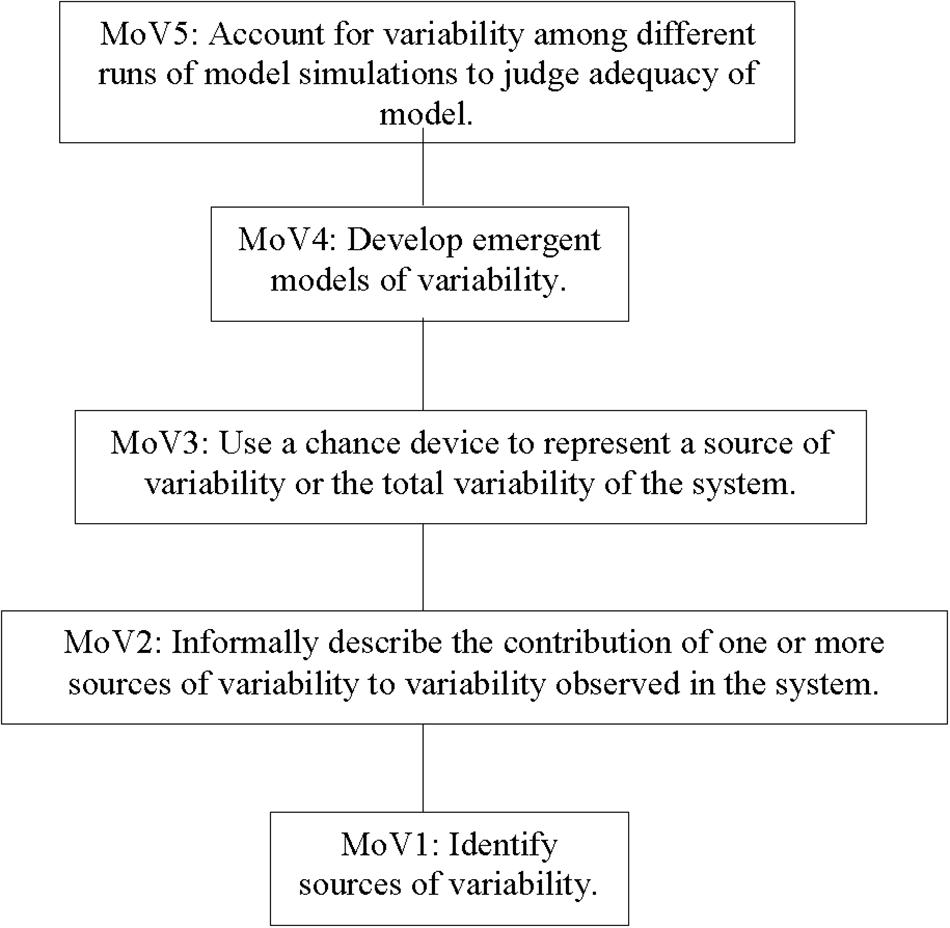
Figure 1. The MoV construct map.

To situate the development and test of this and the five related constructs, we briefly describe the iterative design of the learning progression.

Articulating the Learning Progression

As just noted, the learning progression sought to induct students into an ensemble of approximations to the practices by which professionals come to understand variability, most centrally, on ways to visualize, measure, and model variability. The instruction is designed so that these practices become increasingly coordinated and interwoven over time, so that, for example, initial ways of visualizing data are subsequently employed by students to invent and interpret statistics of sample distribution. The initial construction of the progression involved analysis of core concepts and practices of data modeling (Lehrer and Romberg, 1996) that we judged to be generative, yet intelligible, to students. These were accompanied by conjectures about fruitful instructional means for supporting student induction into ways of thinking and acting on variability that was more aligned with professional practices. One form of conceptual support for learning (a conceptual pivot in the preceding) was a commitment to inducting students into approximations of professional practices through cycles of invention and critique (Ford, 2015). For example, to introduce students to statistics as measures of characteristics of distribution, they first invented a statistic to capture variation in a distribution and then participated in critique during which different inventions were compared and contrasted with an eye toward how they approached the challenges of characterizing variability. It was only after students could participate in such a cycle that conventional statistics of variation were introduced, for now students were in a position to see how conventions resolved some of the challenges revealed by their participation in invention and critique. This participation in practice also helped students understand why there are multiple statistics for characterizing variation in distribution.

Conjectures about effective means for supporting learning were accompanied by development of an assessment system that could be employed for both summative and formative purposes. These assessments provided evidence of student learning that further assisted in the reformation of theory and practice of instruction over multiple iterations of instructional design. The learning progression was articulated during the course of a series of classroom design studies, first conducted by the designers of the progression (e.g., Lehrer et al., 2007, 2011; Lehrer and Kim, 2009; Lehrer, 2017) and subsequently elaborated by teachers who had not participated in the initial iterations of the design (e.g., Tapee et al., 2019). The movement from initial conjectures to a more stabilized progression involved meshing disparate professional communities, including teachers, statisticians, learning researchers, and assessment researchers. Coordination among communities was mediated by a series of boundary objects, ranging from curriculum units to construct maps (such as the one shown in Figure 1) to samples of student work that were judged in relation to professional practices by statistical practitioners (Jones et al., 2017). Teachers played a critical collaborative role in the development of all components of the assessment system, and teacher practices of assessment developed and changed as teachers suggested changes to constructs (e.g., clarifications of descriptions, contributions of video exemplars of student thinking) and items as they changed their instructional practices to use assessment results to advance student learning (Lehrer et al., 2014). Teachers collaborated with researchers to develop guidelines for employing student responses to formative assessments to conduct more productive classroom conversations where students’ ways of thinking, as characterized by levels of a construct, constituted essential elements of a classroom dialog aimed at creating new opportunities for learning (Kim and Lehrer, 2015). During such a conversation, dubbed a “Formative Assessment Conversation” by teachers, teachers drew upon student responses to juxtapose different ways of thinking about the same idea (e.g., a measure of center). Teachers also employed items and item responses as launching pads for extending student conceptions. For example, a teacher might change the nature of a distribution presented in an item and ask students to anticipate and justify effects of this change on sample statistics.

The Six Constructs in the Learning Progression

To describe forms of conceptual change supported by student participation in data modeling practices, we generated six constructs (Lehrer et al., 2014). The constructs were developed during the course of the previously cited design studies which collectively established typical patterns of conceptual growth as students learned to visualize, measure and model the variability generated by processes ranging from repeated measure to production (e.g., different methods for making packages of toothpicks) to organismic growth (e.g., measures of plant growth). Conceptual pivots to promote change, most especially inducting students into statistical practices of visualizing, measuring and modeling variability, were structured and instantiated by a curriculum which included rationales for particular tasks, tools, and activity structures, guides for conducting mathematically productive classroom conversations, and a series of formative assessments that teachers could deploy to support learning.

Visualizing Data

Two of the six constructs represent progression in forms of thinking that typically emerge as students are inducted into practices of visualizing data. Students were inducted into this practice by positioning them as inventors and critics of visualizations of data they had generated (Petrosino et al., 2003). The first, Data Display (DaD), describes conceptions of data that inform how students construct and interpret representations of data. These conceptions are arranged along a dimension anchored by interpreting data through the lens of individual cases to viewing data as distributed—that is, as reflecting properties of an aggregate. At the upper anchor of the construct, aggregate properties constitute a lens for viewing cases. For example, some cases may be more centrally located in a distribution, or some cases may not conform as well as others with properties of the distributed aggregate. A closely associated construct, meta-representational competence (MRC), identifies keystone understandings as students learn to manage representations in order to make claims about data and to consider trade-offs among possible representations in light of particular claims.

Conceptions of Statistics

A third construct, conceptions of statistics (CoS), describes changes in students’ CoS when they have repeated opportunities to invent and critique measures of characteristics of a distribution, such as its center and spread. Initially, students tend to think of statistics not as measures but as the result of computations. For these students, batches of data prompt computation but without sensitivity to the data (e.g., the presence of extreme values) or with a question in mind. As students invent and revise measures of distribution (the invention and critique of measures of distribution is viewed as another conceptual pivot), their CoS encompass a view of statistics as measures, with corresponding sensitivity to qualities of the distribution being summarized, the generalizability of the statistic to other potential distributions, and to the question at hand. The upper anchor of this construct entails recognition of statistics as subject to sample-to-sample variation.

Conceptions of Chance

Chance (Cha) describes the progression of students’ understanding about how elementary probability operates to produce distributions of outcomes. Initial forms of understandings are intuitive and rely on conceptions of agency (e.g., “favorite numbers”). Initial transition away from this agentive view includes the development of the concept of a trial, or repeatable event, as students investigate the behavior of simple random devices. The concept of trial, which also entails abandonment of personal influence on selected outcomes, makes possible a perspectival shift that frames chance as associated with a long-term process, a necessity for a frequentist view of probability (Thompson et al., 2007). Intermediate forms of understandings of chance include development of probability as a measure of uncertainty, and estimation of probabilities as ratios of target outcomes to all possible outcomes of a long-term, repeated process. The upper anchor coordinates sample spaces and relative frequencies as complementary ways of estimating probabilities. Transitions in conceptions of chance are supported by student investigation of the long-run behavior of chance devices, and by the use of statistics to describe characteristics of the resulting distribution of outcomes. A further significant shift in perspective occurs as students summarize a sample with a statistic (e.g., percent of red outcomes in 10 repetitions a 2-color spinner) and then collect many samples. This leads to a new kind of distribution, that of a sampling distribution of sample statistics, and with it, the emergence of a new perspective on statistics as described by the upper anchor of the CoS construct. The constructs of CoS and Cha are related in that the upper anchor of CoS depends upon conceptions of sample-to-sample variation attributed to chance.

Modeling Variability

Building on changing conceptions of chance, the MoV construct posits a progression in learning to construct and evaluate models that include elements of random variation. Modeling chance begins with identification of sources of variability, progresses to employing chance devices to represent sources of variability, and culminates in judging model fit by considering relations between repeated model simulations and an empirical sample. Student conceptions of models and modeling are fostered by positioning students to invent and contest models of processes, ranging from those involving signal and noise, with readily identified sources of variability, to those with less visible sources of variability, as in the natural variation of a sample of organisms.

Informal Inference

The sixth and final construct, Informal Inference (InI), describes transitions in students’ reasoning about inference. The term informal is meant to convey that students are not expected to develop conceptions of probability density and related formalisms that guide professional practice, but they are nonetheless involved in making generalizations or predictions beyond the specific data at hand. The initial levels of the construct describes inferences informed by personal beliefs and experiences in which data do not play a role, other than perhaps confirmation of what one believes. A mid-level of the construct is represented by conceiving of inference as guided by qualities of distribution, such as central clumps in some visualizations or even summary statistics. In short, inference is guided by careful attention to characteristics evident in a sample. At the upper anchor, students develop a hierarchical image of sample in which an empirical sample is viewed as but one instance of a potentially infinite collection of samples generated by a long-term, repeated process (Saldanha and Thompson, 2014). Inference is then guided by this understanding of sample, a cornerstone of professional practice of inference (Garfield et al., 2015).

Generally, the construct maps are psychometrically analyzed and scaled using multidimensional Rasch models (Schwartz et al., 2017), and the requirement relationships are analyzed using structured construct models (Wilson, 2012; Shin et al., 2017).

Checking for Progress: Comparing Pre-Test and Post-Test Results

When conceptualizing and building a learning progression, researchers need to inquire about the extent to which progression-centered instruction influences conceptual change. Constructs inform us about the nature of such change, and pre–post, construct-based assessment informs us about the robustness of the design. In one of the design studies mentioned previously, the project team worked with a sixth-grade teacher to conduct 4 replications of the progression (4 classes taught by the same teacher) with a total of 93 students. The study was aimed at examining variation in student understandings and activity between classes and to gauge the extent of conceptual change for individual students across classes. Students responded to tests taking approximately 1 h to complete before and after instruction. The tests shared only a few items in common, enough to link the two tests together. Item response models (Wright and Masters, 1981) were used to link the scale between the pre-test and the post-test. The underlying latent ability was then used as the metric in which to calculate student gains. This framework allowed us to select a model that accounted for having different items on the forms, varying item difficulty, and different maximum scores of the items.

In the analysis, we used data from both the pre-test and the post-test to estimate the item parameters. We used Rasch models for two reasons: (a) tests that conform to the Rasch model assumptions have desirable characteristics (Wilson, 2005) and (b) the technique of gain scores uses unweighted item scores, and that is satisfied by the Rasch family of models. The estimated item parameters were then used as anchored values and the person ability parameters became the object of estimation. The mean differences between the pre- and post-test were estimated simultaneously with the person and item parameters.

For the scaling model the Random Coefficients Multinomial Logit Model (RCML) (Adams and Wilson, 1996) was used. The usual IRT assumption of having a normal person ability distribution common across both test times is unlikely to be met if indeed the instruction instigates conceptual change, because one would expect to see post-test student abilities that are higher than the pre-test abilities, and this would likely lead to a bi-modal person ability distribution if data from the two tests are combined for analysis. To avoid the unidimensional normality assumption issue, we used a 2-dimensional analysis where the first dimension was the pre-test and the second dimension was the post-test. This can be achieved with a constrained version of the Multidimensional RCML (MRCML) (Adams et al., 1997; Briggs and Wilson, 2003) with common item parameters constrained to be equal across the two dimensions (pre and post). This is a simple example of what is known as Andersen’s Model of Growth (Andersen, 1985). When one constrains the item difficulty of items common to both the pre- and post-test, then the metric is the same for the two test times, and the mean difference between pre- and post-test abilities is the gain in ability between the two tests (Ayers and Wilson, 2011). The MRCML model was designed to allow for flexibility in designing custom models and is the basis for the parameter estimation in the ConQuest software (Adams et al., 2020). We formulated the MRCML as a Partial Credit Model (PCM) (Masters, 1982) and used the within-items form of the Multidimensional PCM, as each common item loads onto both the pre-test and the post-test dimension.

Results from the ConQuest analysis are summarized in Table 1. In particular, we focus on MoV, as above, for illustrative purposes: the mean ability gain for MoV was 1.312 logits. In order to test if the difference between the post-test ability and the pre-test ability is statistical significant, we used a Wald test

TABLE 1

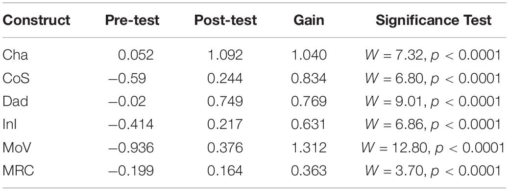
Table 1. Pre- and post-test mean ability estimates, gain scores, and Wald test significance results.

$$W=\frac{({\widehat{\mathrm{\mu }}}_{post}-{\widehat{\mathrm{\mu }}}_{pre})}{\sqrt{\frac{s_{pre}^2}{N}+\frac{s_{post}^2}{N}}},(1)$$

where _{${\widehat{\mathrm{\mu }}}_{pre}$, ${\widehat{\mathrm{\mu }}}_{post}$, $s_{pre}^2$,} and _{$s_{post}^2$} are the sample means and variance and N is the sample size. A size α Wald test rejects the null hypothesis (of no difference) when | W| > z_α/2. Row 5 in Table 1 shows the results for the MoV construct. Column 1 indicates the construct, columns 2–4 indicate the mean pre-test ability, mean post-test ability, and the gain, and column 5 shows the Wald test statistic and the p-value when using α = 0.05. For MoV, the test statistic is W = 12.80 and p < 0.0001. Thus, we can reject the null hypothesis and conclude that the post-test ability is significantly higher than the pre-test ability. The other rows show the results for the remaining five constructs. In each case the p-value is less than 0.0001 and thus we have statistically significant gains.

In addition to statistical significance, it is important to gauge effect size—that is, are the gains large enough to claim that these are important effects? In our studies of scaling educational achievement tests, we have found from experience that, looking at similar achievement tests, typical differences in achievement test results from 1 year to the next are approximately 0.3–0.5 logits [see for example, Wilson et al. (2019a) and Wilson et al. (2012)]. Hence, we see these gains (which are greater than half a logit for all but one of the constructs) as representing very important gains over the briefer (7–8 weeks) period of instruction in data modeling.

With this summative illustration in mind, we turn now to some of its underpinnings and to the use of assessments by teachers. In what follows, we focus on one particular construct from among the six in the full Data Modeling learning progression, MoV, and describe (a) the development of assessments based on the construct maps, and their relationships with instruction by teachers, (b) the development of empirical maps of these constructs (referred to as “Wright maps”), and (c) the usages of reports based on these maps by teachers.

A Closer View of a Construct: Modeling Variability

As noted previously, the MoV construct refers to the conceptions and practices of modeling variability. Modeling-related concepts emerge as students participate in curricular activities designed to make the role of models in statistical inference visible and tractable. In professional practice, models guiding inference rely on probability density functions, but we take a more informal approach (see Lehrer et al., 2020 for a more complete description). One building block of inference is an image of variable outcomes that are produced by the same underlying process. Accordingly, we first have students use a 15 cm ruler to measure the length of the same object, such as the perimeter of a table or the length of their teacher’s outstretched arms. Much to their surprise, students find that if they have measured independently, their measures are not all the same, and furthermore, the extent of variability is usually substantially less when other tools, such as a meter stick, are used. Students’ participation informs their understanding of potential sources of differences observed, which tend to rely on perceptions of signal (the length of the object) and noise (“mistakes” measurers made arising from small but cumulative errors in iterating the ruler or from how they treated the rounded corners of a table, etc.). A signal-noise interpretation is a conceptual pivot in that it affords an initial step toward understanding how sample variability could arise from a repeated process. And, the accessibility of the process of measuring allows students to make attributions of different sources of error—a prelude to an analysis of variance. The initial seed of an image of a long-range process, so important to thinking about probability and chance, is systematically cultivated throughout the curricular sequence. For example, as students invent visualizations of the sample of measured values of the object’s length, many create displays of data that afford noticing center clumps and symmetries of the batch of data. This noticing provides an opportunity for teachers to have students account for what they have visualized. For example, what about the process tends to account for center clump and symmetry? Students critique their inventions with an eye toward what different invented representations tend to highlight and subdue about the data, so that the interplay between invention and critique constitute opportunities for students to develop representational and metarepresentational competencies, which are described by the two associated constructs DaD and MRC.

Students go on to invent measures of characteristics of the sample distribution, such as an estimate of the true length of the object (e.g., sample medians) and the tendency of the measurers to agree (i.e., precision of measure). Invented statistics are critiqued with an eye toward what they attend to in the sample distribution and what might happen if the distribution were to be transformed in some way (e.g., sample size increased). Invention and critique help make the conceptions and methods of statistics more intelligible to students, and transitions in students’ conceptions are illustrated by the CoS construct. After revisiting visualizing and measuring characteristics of distributions in other signal-noise contexts (e.g., manufacturing Play-Doh candy rolls), students grapple with chance by designing chance devices and observing their behavior. The conceptual pivot of signal and noise comes into play with the structure of the device playing the role of signal and chance deviations from this structure playing the role of noise. Changes in conceptions of chance that emerge during the course of these investigations are described by the Cha construct and by upper anchor of the CoS construct.

With this conceptual and experiential grounding, students are challenged to invent and critique MoV producing processes that now include chance. Initially, models are devoted to re-considerations of signal and noise processes from the perspective of reconsidering mistakes as random—for instance, despite being careful, small slippages in iteration with a ruler over a long span appear inevitable and also unpredictable. Accordingly, the process of measuring an object’s length can be re-considered as a blend of a fixed value of length and sources of random error. As students invent and critique MoV in contexts ranging from signal and noise processes to those generating “natural” variation, they have opportunities to elaborate their conceptions of modeling variability.

Modeling Variability (MoV)

With the preceding in mind, we can now describe the MoV construct and its construct map—refer to Figure 1 for an outline. Students at the first level, MoV1, associate variability with particular sources, which is facilitated by reflecting on processes characterized by signal and noise For example, when considering variability of measures of the same object’s length, students may consider variability as arising from misdeeds of measurement, “mistakes” made by some measurers because they were not “careful.” To be categorized at this initial level, it is sufficient that students demonstrate an attribution about one or more sources of variability but not that they implicate chance origins to variability.

At level MoV2, students begin to informally order the contributions of different sources to variability, using language such as “a lot” or “a little.” They refer to mechanisms and/or processes that account for these distinctions, and they predict or account for the effects on variability of changes in these mechanisms or processes. For example, two students who measured the perimeter of the same table attributed errors to iteration, which they perceived as substantial. Then, they went on to consider other errors that might have less impact, such as a “false start.” This conversation clarifies that students need to clarify the nature of each source of variability and decide whether or not the source is worthy of including in a model.

Cameron: How would we graph–, I mean, what is a false start, anyway?

Brianna: Like you have the ruler, but you start at the ruler edge, but the ruler might be a little bit after it, so you get, like, half a centimeter off.

Cameron: So, then it would not be 33, it’d be 16.5, because it’d be half a centimeter off?

Brianna: Yeah, it might be a whole one, because on the ruler that we had, there was half a centimeter on one side, and half a centimeter on the other side, so it might be 33 still, and I think we subtract 33.

Cameron: Yeah, because if you get a false start, you’re gonna miss (Lehrer et al., 2020).

An important transition in student reasoning occurs at level MoV3: here students explicitly consider chance as contributing to variability. In the curricular sequence, students first investigate the behavior of simple devices for which there is widespread acknowledgment that the behavior of the device is “random.” For example, consider the spinner illustrated in the top panel of Figure 2. This is a blank (“mystery”) spinner, and the task for the student is to draw a line dividing the spinner into two sectors which indicate the two proportions for the outcomes of the spinner, which are given in the lower panel. The conceptual consequences of investigations like these are primarily captured in the Cha construct, but from the perspective of modeling, students come to appreciate chance as a source of variability.

FIGURE 2

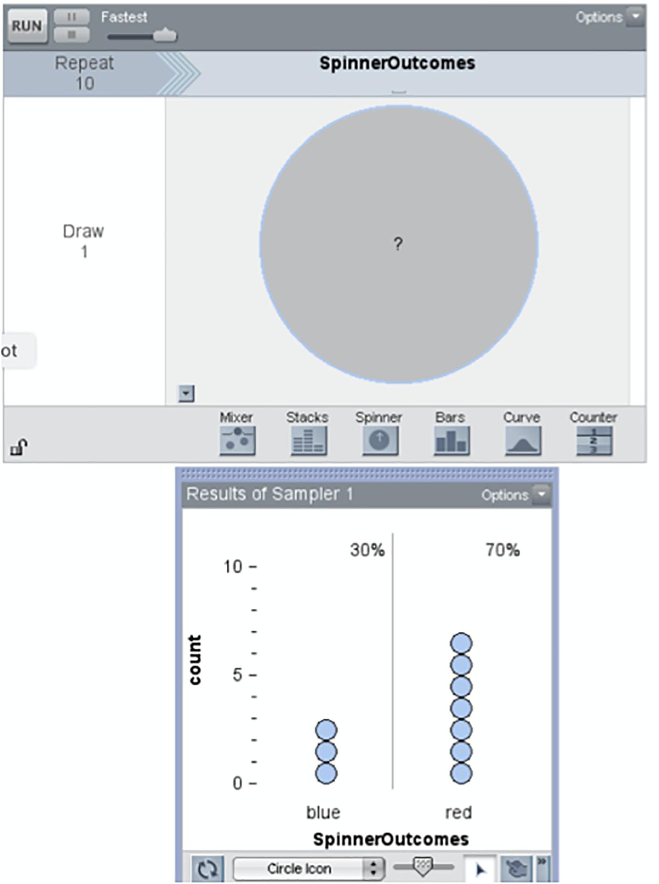
Figure 2. Representation of a “mystery” spinner.

At level MoV4, there is a challenging transition to conceptualizing variability in a process as emerging from the composition of multiple, often random sources. For example, a distribution of repeated measurements of an attribute of the same object can be modeled as a composition of a fixed or true measure of the attribute and one or more components of chance error in measure. Figure 3 illustrates a student-generated model that approximates the variability evident in a sample of class measures of the length of their teacher’s arm-span. In this Figure, the spinners are ordered from left to right, and are labeled above each with a 3-letter code, described below. The first spinner (labeled MDN) is simply the sample median of the observed sample, taken by the students as their “best guess of” the true value of the teacher’s arm-span—this is a deterministic effect, as represented by the fact that there is only one sector in the spinner, so it will return the same value (i.e., 157) on each spin. The remaining four spinners are all modeling random effects, as they will return different values on each spin, with probability proportional to the proportion of the spinner area occupied by each sector¹. The second spinner (labeled GAP) represents the “gaps” that occur when students iterate application of their rulers across the teacher’s back: the probabilities of these gaps are proportional to the areas of the spinner sectors, and the values that are returned are shown within each sector (i.e., −1 to −9). The students had surmised that smaller magnitudes of the gaps are more likely to occur than larger magnitudes, hence the sectors vary in area, reducing from the area for −1 to the area for −9. The values are negative because gaps are unmeasured space and hence result in underestimates of the arm-span. The third spinner (labeled LAP) represents the “overlaps” that occur when the endpoint of one iteration of the ruler overlaps with the starting point of the next iteration. The interpretation of the values and sectors is parallel to that for GAP. The values are positive value because this mistake creates overestimates of the measure (i.e., the same space is counted more than once). The fourth spinner (labeled Droop) represents both under- and over-estimates—these result when the teacher becomes tired and her outstretched arms droop. The last spinner (labeled Whoops) represents probabilities and values of mis-calculations when each student generated a measure. The way the whole spinner device works is that the result from each spinner is added to a total to generate a single simulated measurement value. This then can be used to generate multiple values for a distribution (students typically used 30 repetitions in the Data Modeling curriculum because these corresponded to the number of measurers). MoV4 culminates with the capacity to compare two or more emergent models, a capacity which is developed as students critique models invented by others.

FIGURE 3

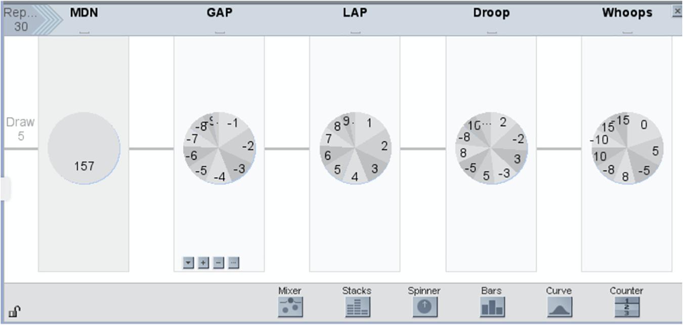
Figure 3. Modeling variability as a composition of signal and multiple sources of random error.

At level MoV5, students consider variability when evaluating models. For example, they recognize that just by chance one run of a model’s simulated outcomes may fit an empirical sample well (e.g., similar median and IQR values, similar “shapes” etc.) but the next simulated sample might not. So, students, often prompted by teachers to think about running the simulations “again and again” begin to appreciate the role of multiple runs of model simulations to judge the suitability of the model. Sampling distributions of estimates of model parameters, such as simulated sample median and IQR, are used to judge whether or not the model tends to approximate characteristics of an empirical sample at hand. This is a very rich set of concepts for students to explore, and, eventually, grasp. Just one example of this richness is indicated by a classroom discussion of the plausibility of sample values that were generated by a model, but which were absent in the original empirical sample. The argument for and against a model that could generate such a value arose during a formative assessment, and as in other formative assessments, the teacher conducted a follow-up conversation during which different student solutions were compared and contrasted to instigate a transition in student thinking, here from MoV4 to MoV5. As the teacher anticipated, some students immediately objected to model outcomes not represented as cases in the original sample. They proposed a revision to the model under consideration by the class which would eliminate this possibility.

Students: Take away−1 in the spinner

Teacher: Why?

Joash: Because there’s no 9 in this [the original sample].

But another student, Garth, responded, “Yeah, but that doesn’t mean 9 is impossible.” He went on to elaborate, that the model was “focused on the probability of messing up,” so to the extent to which error magnitudes and probabilities were plausible, they should not be excluded, and one would have to accept the simulated values generated by the model as possible values (Lehrer et al., 2020). This discussion of “possible values” eventually assumed increasing prominence among the students, and led to a point where they began to consider empirical samples as simultaneously (a) a collection of outcomes observed in the world and (b) a member of a potentially infinite collection of samples (Lehrer, 2017). As mentioned previously, this dual recognition of the nature of a sample is an important seed stock of statistical inference.

Building an Assessment System in the Context of a Construct Map

Having achieved this initial step of generating a construct map that reflected benchmarks in students’ conceptions of modeling variability, we designed an assessment system to provide formative feedback to teachers to help them monitor student progress and also to provide summative assessment for other classroom and school uses. In practice, design and development of the assessment system paralleled that of the development of the curricular sequence, albeit with some lag to reflect upon the robustness of emerging patterns of student thinking. In this process, we follow Wilson’s (2005) construct-centered design process, the Bear Assessment System (BAS), where items are designed to measure specific learning levels for the construct, where item modes include both multiple choice and constructed response types. The student responses to the constructed response items are first mined to develop scoring guidelines consisting of descriptions of student reasoning and to provide examples of student work, all aligned to specific levels of performance. This process involved multiple iterations of item design, scoring, comparison of the coded responses to the construct map, then fitting of items to psychometric models using the resulting data, and subsequent item revision/generation. These iterations occur over fairly long periods, and are based on the data from students across multiple project teachers—these teachers have variable amounts of expertise, but were all engaged in the professional development that was an inherent part of being a member of that team. The review teams included the Vanderbilt project leaders, who, along with other colleagues, were working directly with teachers. This brought the instructional experiences of teachers into the process, and, for some issues that arose, teachers proposed and tried out new approaches. Sometimes, due to patterns in student responses, we refined construct map levels and/or items, and coding exemplars, including re-descriptions of student reasoning and inclusion of more or better examples of student work (Constructs were also revised to make them more intelligible and useful for guiding instruction in partnership with teachers, as suggested earlier). New items were developed where we found gaps in coverage of the landmarks in the roadmap of student learning described by the construct. In the light of student responses, some items that could not be repaired were discarded, others were redesigned to generate clearer evidence of student reasoning. Sometimes, student responses to items could not be identified as belonging to the construct but nonetheless appeared to indicate a distinctive and important aspect of reasoning: This led to revision of constructs and/or levels. A much more detailed explanation of this design approach to developing an assessment system is given in Wilson (2005).

Example Item 1—Piano Width

To illustrate the way that items are matched to construct map levels, consider the Piano Width task illustrated in Figure 4. This task capitalizes on the Data Modeling student’s experiences with ruler iteration errors (“gaps and laps”) in learning about measurement as a process that generated variability. We comment specifically on question 1 of the Piano Width item: The first part–1(a)—is intended mainly to have the student adopt a position, and is coded simply as correct or incorrect. The interesting question, as far as the responses is concerned, is the second part–1(b)—here the most sophisticated responses are at the MoV2 level, and typically fall into one of two categories after choosing “Yes” to question 1(a).

FIGURE 4

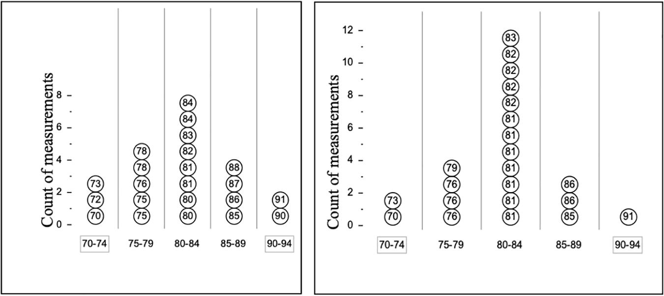
Figure 4. The Piano Width item. A group of musicians measured the width of a piano in centimeters. Each musician in this group measured using a small ruler (15 cm long). They had to flip the ruler over and over across the width of the piano to find the total number of centimeters. A second group of musicians also measured the piano’s width using a meter stick instead. They simply laid the stick on the piano and read the length. The graphs below display the groups’ measurements. 1(a) The two groups used different tools. Did the tool they used affect their measurement? (check one) () Yes () No. 1(b) Explain your answer. You can write on the displays if that will help you to explain better. 2(a) How does using a different tool change the precision of measurements? (check one). (a) Using different tools does not affect the precision of measurements. (b) Using the small ruler makes precision better. (c) Using the meter stick makes precision better. 2(b) Explain your answer. (What about the displays makes you think so?).

MOV2B: the student describes how a process or change in the process affects the variability, that is, the student compares the variability shown by the two displays. The student mentions specific data points or characteristics of the displays. For example, one student wrote: “The Meter stick gives a more precise measurement because more students measured 80–84 with the meter stick than with the ruler.”

MOV2A: the student informally estimates the magnitude of variation due to one or more sources, that is the student and mentions sources of variability in the ruler or meter stick. For example, one student wrote: “The small ruler gives you more opportunities to mess up.”

Note that this is an illustration of how the construct map levels may be manifested into multiple sub-levels, and, as in this case, there may be some ordering among the sublevels (i.e., MoV2B is seen as a more complete answer than MoV2A).

Less sophisticated responses are also found:

MOV1: the student attributes variability to specific sources or causes, that is the student chooses “Yes” and attributes the differences in variability to the measuring tools without referring to information from the displays. For example, one student wrote: “The meterstick works better because it is longer.”

Of course, students also give unclear or irrelevant responses, such as the following: “Yes, because pianos are heavy”—these are labeled as “No Link(i),” and abbreviated NL(i). In the initial stages of instruction in this topic, students also gave a level of response that is not clearly yet at level MoV1, but was judged to be better than completely irrelevant—typically these responses contained relevant terms and ideas, but were not accurate enough to warrant labeling as MoV1. For example, one student wrote: “No, Because it equals the same” This scoring level was labeled “No Link(ii)” and abbreviated NL(ii), and was placed lower than MoV1. Note that a complete scoring guide for this task is shown in Appendix A.

An Empirical Version of the Learning Construct—The Wright Map

We used a sample of 1002 middle school students from multiple school districts involved in a calibration of the learning progression, which included (a) generation of tools to support professional development beyond the initial instantiations of the progression, most especially collaboration with teachers to develop curriculum and associated materials, (b) expansion of constructs to include video exemplars (Kim and Lehrer, 2015), and (c) item calibration (Schwartz et al., 2017), all of which were conducted prior to implementation of a cluster randomized trial. In a series of analyses carried out before the one on which the following results are based, we investigated rater effects for the contructed response items, and no statistically significant rater effects were found, so these are not included in the analysis. We fitted a partial-credit, one-dimensional item response (IRT) model, often termed a Rasch model, to the item responses related to the MoV construct. This model distinguishes among levels of the construct (Masters, 1982). For each item, we use threshold values (also called “Thurstonian thresholds”) to describe the empirical characteristics of the item (Wilson, 2005; Adams et al., 2020).

The way that the item is represented is as follows:

(a) if an item has k scoring levels, then there are k-1 thresholds on the Wright map, one for each transition between scores;

(b) each item threshold gives the ability level (in logits) that a student must obtain to have a 50% chance of scoring at the associated scoring category or above (The locations of these thresholds for the MoV items are shown in the columns on the right side of Figure 5—more detail below).

FIGURE 5

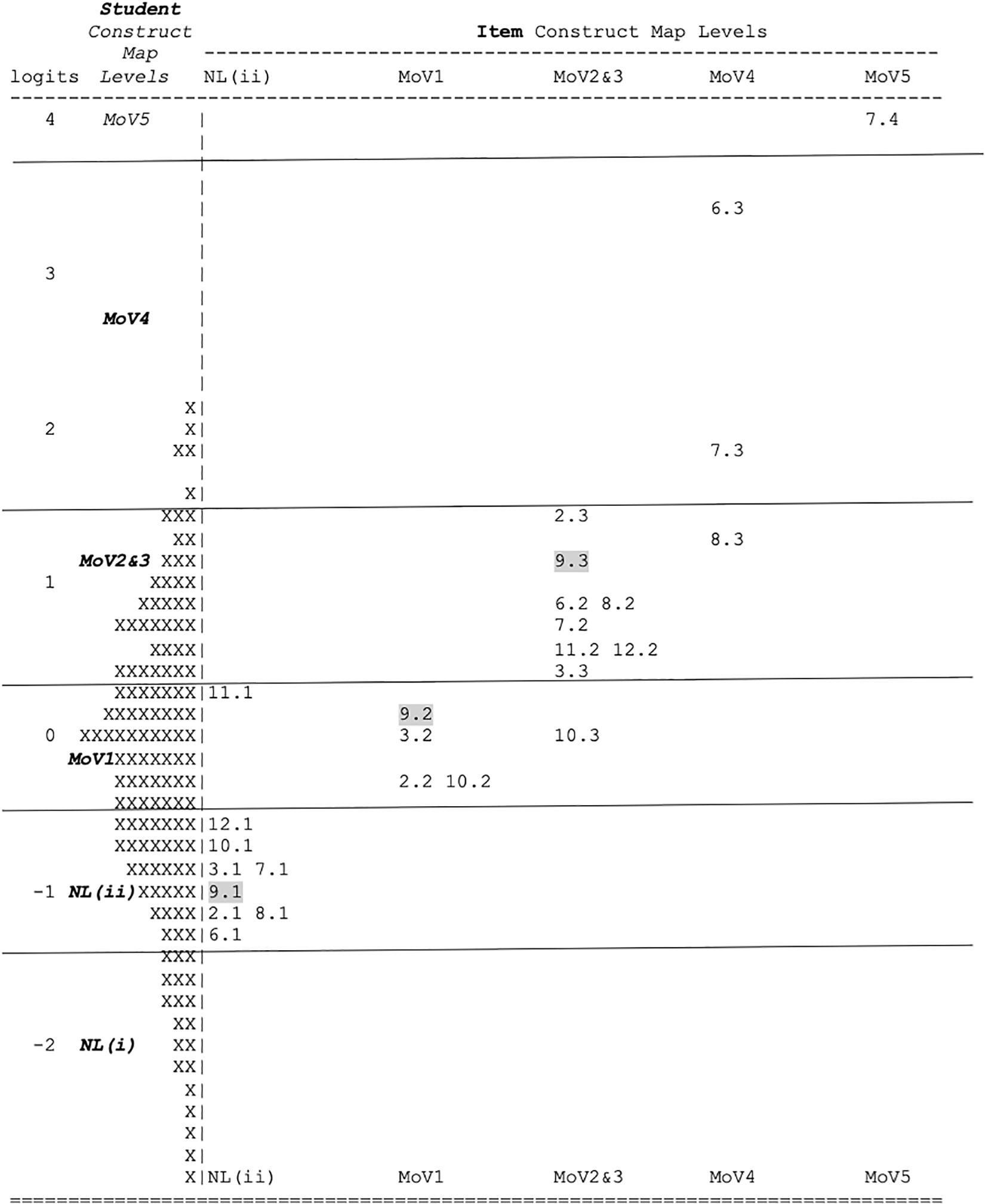
Figure 5. The Wright Map for MoV.

For example, suppose an item has three possible score levels (0, 1, and 2). In this case there will be two thresholds. Suppose that the first threshold has a value of −0.25 logits: This means that a student with that same ability of −0.25 has an equal chance of scoring in category 0 compared to categories 1 and 2. If their ability is lower than the threshold value (−0.25 logits), then they have a higher probability of scoring in category 0; if their ability is higher than −0.25, then they have a higher probability of scoring in either category 1 or 2 (than 0). These thresholds are, by definition, ordered: In the given example, the second threshold value must be greater than −0.25. Items may have just one threshold (i.e., dichotomous items, for example, traditional multiple-choice items), or they can be polytomous. It would be very transparent if every item had as many response categories as there are construct map levels–however, this is often not the case–sometimes items will have response categories that focus only on a sub-segment of the construct, or, somewhat less commonly, sometimes items will having several different response categories that match to just one of the levels of a construct map. For this reason, it is particularly important to pay careful attention to how item response categories can be related to the levels of the construct map.

The locations of the item thresholds can be graphically summarized in a Wright map, which is a graph that simultaneously shows estimates for both the students and items on the same (logit) scale. Figure 5 shows the Wright Map for MoV, with the thresholds represented by “i.k,” where i is the item number and k is the threshold number, so that, say, “9.2” stands for the second threshold for the 9th item. On the left side of the Wright Map, the distribution of student abilities is displayed, where ability entails knowledge of the skills and practices for MoV. The person abilities have a roughly symmetric distribution. On the right side are shown the thresholds for 9 questions from 5 tasks in MoV. In Figure 5, the thresholds for Piano Width questions 1(b) and 2(b) are labeled as 9.k and 10.k, respectively. Again, focussing on question 1(b) (item 9), the thresholds (9.1, 9.2, and 9.3) were estimated to be −0.97, 0.16, and 1.20 logits, respectively. Looking at Figure 5, one can see that they stand roughly in the middle of the segments (indicated by the horizontal lines) of the logit scale for the NL(ii), Mov1 and MoV2&3 levels, respectively.

Looking beyond a single item, we need to investigate the consistency of the locations of these thresholds across items. We used a standard-setting procedure called “construct mapping” (Draney and Wilson, 2011) to develop cut-scores between the levels. Following that process, we found that the thresholds fall quite consistently into the ordered levels, with a few exceptions, specifically 8.3, 10.3, and 11.1. In our initial representations of this Wright map, we found that the thresholds for levels 2 and 3 were thoroughly mixed together. We spent a large amount of time exploring this, both quantitatively, using the data, and qualitatively, examining item contents, and talking to curriculum developers and teachers about the apparent anomaly. Our conclusion was that these two levels, although there is certainly a necessary hierarchy to their lower ends—there is little hope for a student to use a chance devise to represent a source of variability (MoV3) if they cannot informally describe such a source (MoV2)—and these can and do overlap quite a bit in the classrooms of the project. Students are still improving on MoV2 when they are initially starting on Mov3, and they continue to improve on both at about the same time. Hence, at least formally, that, while we decided to uphold the distinction between Mov2 and MoV3, we also decided to ignore the difference in difficulty of the levels, and to label the segment of the scale (i.e., the relevant band) as MoV2&3. Thus, our MoV construct map may be modified as in Figure 6.

FIGURE 6

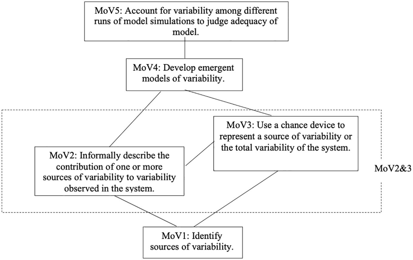
Figure 6. The Revised MoV construct map.

These band-segments can then be used as a means of labeling estimated student locations with respect to the construct map levels NL(i) to MoV4. For example, a student estimated to be at 1.0 logits could be interpreted as being at the point of most actively learning (specifically, succeeding at the relevant levels approximately 50% of the time) within the construct map levels MoV2 and MoV3, that is, being able to informally describe the contribution of one or more sources of variability to the observed variability in the system, while at the same time developing a chance device (such as a spinner) to represent that relationship. The same student would be expected to succeed more consistently (approximately 75%) at level MoV1 (i.e., being able to identify sources of variability), and succeed much less often (approximately 25%) at level MoV4 (i.e., develop an emergent model of variability). Thus, the average gain of the students on the Modeling Variability construct, as reported above (1.312 logits) was, in addition to being statistically significant, also educationally meaningful, representing approximately a difference of a full MoV construct level.

Using the Bass System to Implement the Assessments in the Learning Progression

The components of the assessment system, as shown above, including the construct maps, the items, and the scoring guides, are implemented within the online Bear Assessment System Software (BASS), which can deliver the items, automatically score those designed that way (or manage a hand-scoring procedure for items designed to be open-ended), assemble the data into a manageable data set, analyze the data using Rasch-type models according to the designed constructs, and report on the results, in terms of (a) a comprehensive analysis report, and (b) individual and group results for classroom use (Torres Irribarra et al., 2015; Fisher and Wilson, 2019; Wilson et al., 2019b). In this account, we will not dwell on the structures and features of this program, but will focus instead on those parts of the BASS reports that will be helpful to a teacher involved in teaching based on the MoV construct.

Figure 6 gives an overall empirical picture of the MoV construct, and this is also the starting point for a teacher’s use of the software². This map shows the relationship between the students in the calibration sample for the MoV construct and the MoV items, as represented by their Thurstone thresholds. The thresholds span across approximately 5 logits, and the student span is about the same, though they range about 1.5 logits lower. This is a relatively wide range of probabilities of success—for a threshold located at 0.0 logits, a student at the lowest location will have approximately a 0.05 chance of achieving at that threshold level: in contrast, a student at the highest location will have approximately a 0.92 chance of achieving at that threshold level. This very wide range reflects that this construct is not one that is commonly taught in schools, so that the underlying variation is not much influenced by the effects of previous instruction. This is a sobering challenge for a teacher—how to educate both the students who are working at the NL(i) level, not even being able to write down appropriate words in response to the items, and the students who are working at the Mov4 level, where they are able to engage in debates about the respective qualities of different probabilistic models.

Of course, no real class will have such a large number of students to contend with, so we have illustrated the equivalent map to Figure 5 for two different classes in Figure 7—Class I and Class II. These each represent the results for a whole school rather than for a single classroom, so should be interpreted as a group of students who might be spread across several individual classrooms. The class whose distribution is shown on the far left of the logit scale in Figure 7 is representative of students before systematic instruction in modeling variability. The majority of students are at either level NL(i) or NL(ii), and hence, that there has been little successful past instruction on this topic. Nevertheless, we can see that here are a few students who are working at the lower ends of MoV2&3, that is they can recognize that there is qualitative ordering of the effects of different sources of variation, and are beginning to be able to understand how these might be encapsulated in a model based on chance. Now, contrast that with the class (Class II) whose distribution is shown immediately to the right of Class I in Figure 7. Here the whole distribution has moved up by approximately a logit, and hence, the number of students at that lowest level (NL(i) are very few. The largest group in this class is at the level MoV1, that is they can express their thinking about possible sources of variation, and a few students are beginning to operate at the highest level we observed, MoV4. This class is representative of students with some experience with constructing models but likely not with extensive opportunities to invent and revise models across multiple variability-generating contexts. This broad envisioning of the educational challenge of the classes (i.e., the range of the extant construct levels) allows a teacher to anchor their instructional planning in reliable information on student performance on an explicitly known (to the teacher) set of tasks.

FIGURE 7

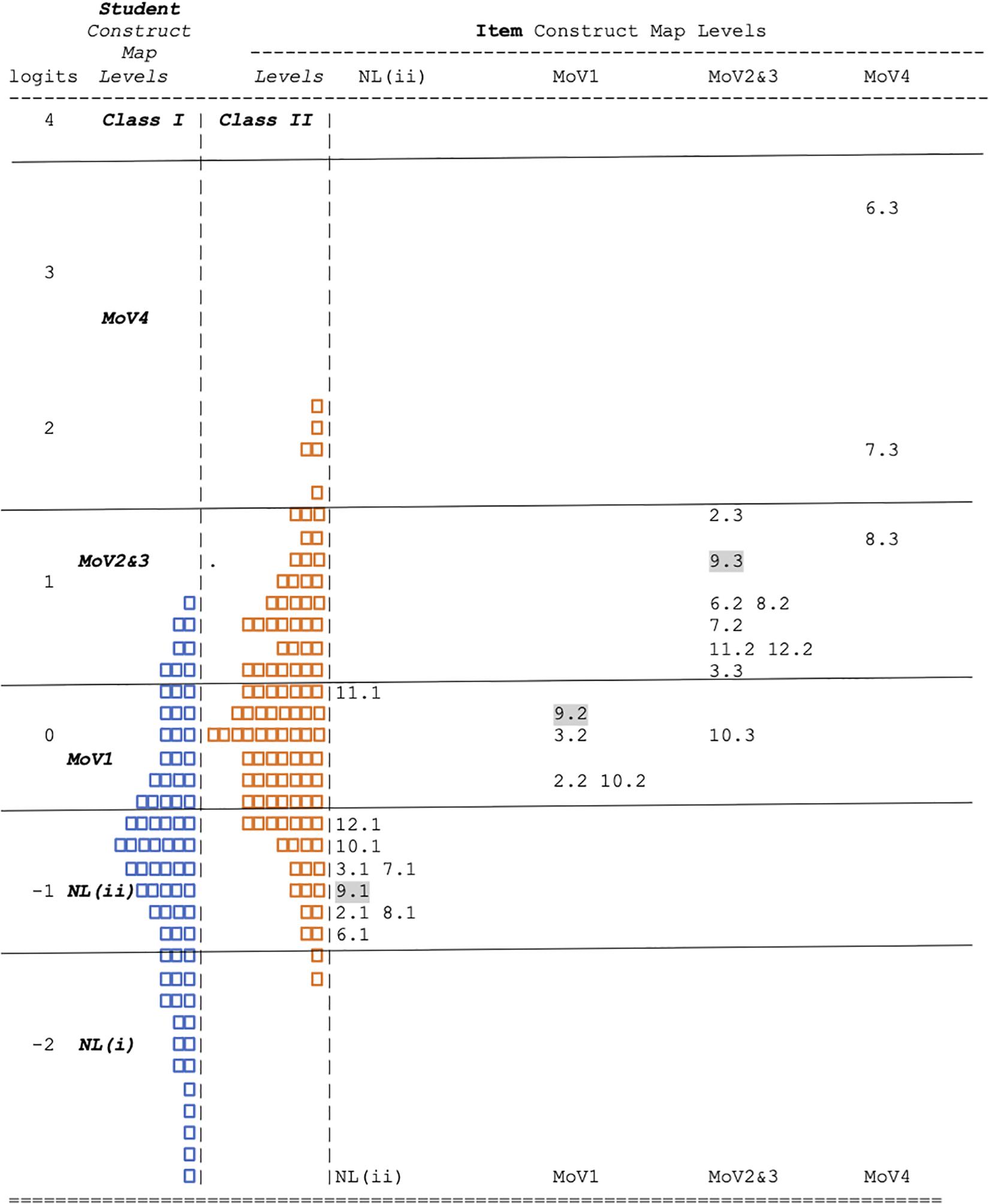
Figure 7. The Wright Map for MoV: Class I (left) and II (right). Each box represent approximately 1 case: 102 altogether.

Turning now to specific interpretive and diagnostic information that a teacher can gain from the system, consider an individual student report, as shown in Figure 8. Here we see that this student (anonymously labeled as “Ver1148” in this paper) is doing moderately well in the calibration sample—(s)he is most likely located in the Mov2 level (the 95% confidence interval is indicated on the graph by the horizontal bars around the central dot). This information provides some useful educational possibilities for what next to do with this student—they should continue practicing the informal observation and description of sources of variability, and they should be moving on to learn about how to use a chance device to represent the probabilities.

FIGURE 8

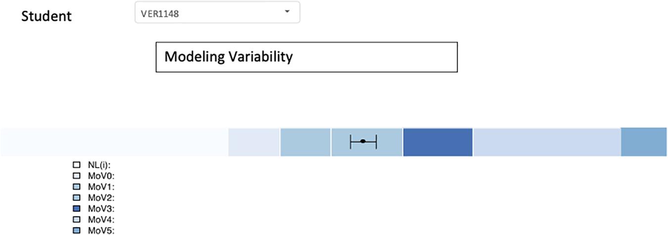
Figure 8. A BASS report on the performance of an individual student on the MoV items set.

Individual student reports can also assist teachers to use an item formatively by juxtaposing student solutions at adjacent levels of the construct, and inviting whole-class reflection as means to help students to extend their reasoning to higher levels of the construct (Kim and Lehrer, 2015). The formative assessment conversation described previously during the presentation of MoV5 exemplifies this adjoining construct level heuristic. In that conversation, the teacher invited contrast between student models that emphasized recapitulation of values observed in a single sample (a MoV4 level) with a model that instead allowed for values plausibly reflecting the variability-generating process (“possible values”), which reflected the emphasis on sampling variability characteristic of MoV5.

The teacher can also look more deeply into a student’s record for the construct, and examine their performance at the item level. This is illustrated in Figure 9, where the student’s responses for each item that the teacher chose for the student’s class are shown graphically–this shows exactly which responses (s)he gave to each item, and matches them to the construct map levels (i.e., with the items represented in the rows and the construct map levels are illustrated in the columns). Here it can be seen³ that the item-level results are quite consistent with the overall view as given in Figure 5—with the student performing with a moderate level of success on the MoV2 items (i.e., the last 3), and doing as well as can be expected on the first 3 items, which do not prompt responses for levels 1 or 2.

FIGURE 9

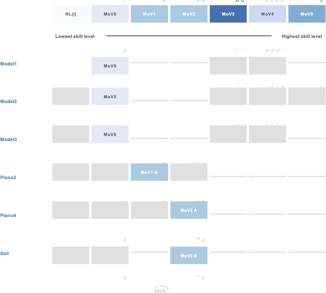
Figure 9. A BASS item scores report for an individual student on the MoV items set.

Of course, not every student will give results that are so consistent with the expected order of items in the Wright Map. This is educationally relevant, as performances that are inconsistent with the usual may indicate that the student has special interests, experiences, or even attitudes that should be considered in interpreting their results. We use a special type of graphical display, called a “kidmap,” that can make this clearer (although like any other specialist figure, it does need explanation). The kidmap for student Ver1148 is shown in Figure 10. The student’s location on the map is shown as the horizontal line marked with their identifier in the middle of the figure. The logit scales to the left and right of this show, respectively, (a), to the left, the construct map levels that the student achieved, and (b), to the right, those that the student did not achieve. The extent of the measurement error around the student location is marked by the blue band around the horizontal line. The way to read the graph is to note that, when the student has performed as expected by his overall estimated location, then

FIGURE 10

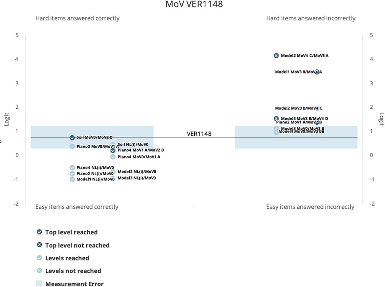
Figure 10. A Kidmap report for an individual student on the MoV items set.

(a) the construct map levels achieved should show up in the bottom left-hand quadrant of the graph,

(b) the construct map levels not achieved should show up in the top right-hand quadrant of the graph, and

(c) there may be a region of inconsistency within and/or near to the region of uncertainty (i.e., the blue band).

In fact, looking at Figure 10, we can see that this student’s performance is very much consistent with their estimated location, there are no construct map levels showing up in the “off” diagonal; quadrants (top left and bottom right).

To illustrate the way that this type of graph can help identify student performances that are inconsistent with their overall estimated location, look now at Figure 11. In this kidmap, for student Ver1047, we can see that the “off-diagonal” quadrants are indeed occupied by a number of item levels. Those in the top left quadrant are those for which the student has performed better that their overall estimate would predict, while those in the bottom right quadrant are those for which the student did not perform as well as expected. This can them be interpreted very specifically by examining the student scores output shown in Figure 12. Here it can be readily seen that this student has performed very inconsistently on the item that the teacher assigned, responding at a high level (MoV4) for the first 3 items and at the lowest level (NL(i)) for the last three items. An actual interpretation of these results would require more information about the student and the context—nevertheless, it is important that the teacher be made aware of this sort of result, as it may be very important for the continued success of this individual student. Fortunately, cases such as that for Ver1148 can be readily detected by using a “Person Misfit” index, thus avoiding the need for a teacher to examine the kidmaps for every one of their students—this is also reported for each student by BASS. This type of result, where the student’s response vector can be used as a form of quality control information on the overall student estimate, is an important step forward in assessment practice—giving the teacher potential insights into the way that students have learned the content of instruction.

FIGURE 11

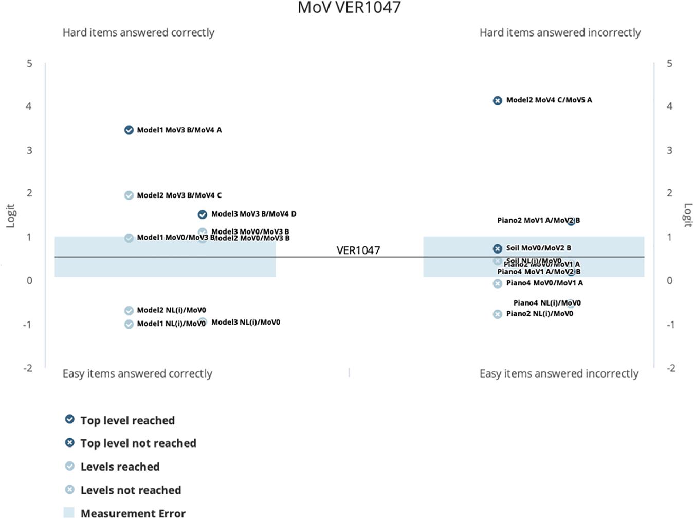
Figure 11. A Kidmap report for a second individual student on the MoV items set.

FIGURE 12

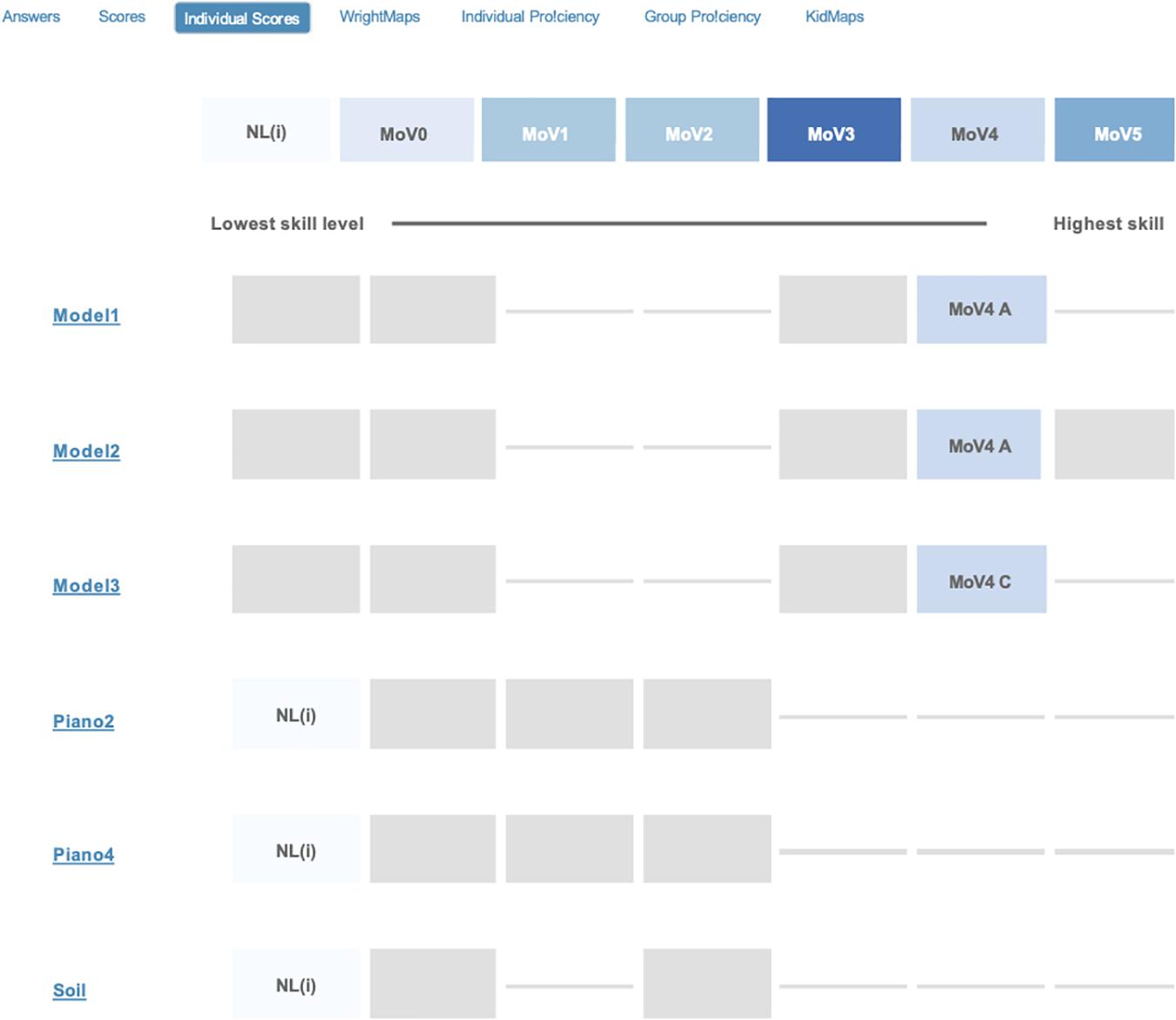
Figure 12. A BASS item scores report for a second individual student on the MoV items set.

Conclusion

This paper has described how a learning progression can be defined using benchmarks of conceptual change and in tandem, conceptual pivots that may instigate change. These together characterize the structural components of the learning progression. The assessment aspect of the progression has been characterized using constructs and their accompanying construct maps, which serve multiple purposes: as ways to highlight and describe anticipated forms of student learning, as a basis for recording and visualizing progress in student learning, and as a method to link assessment with instruction. Instruction is intertwined with assessment in ways that are manifest in the structure of the assessment system, as in the negotiation of the representation of constructs in ways that teachers find useful, intelligible, and plausible, and in the practice of assessment, where teachers use formative items to advance learning by engaging students in productive, construct-centered conversation.

Next Steps

The next major steps in continuing the assessment work described here are the following. In the first step, the many constructed response items in the DM item bank, such as the one used as an example above, need to be augmented with similar selected response items. The selected response versions can be developed from the responses collected as part of the calibration of the open ended responses. These selected response items are crucially needed in order to lighten the load on teachers so that they can avoid having to score the open ended responses that their students make. The aim, however, is not to then ignore the open ended items, but to preserve both formats in the DM item bank so that the open ended ones can be used for instructional purposes as well as informal assessments, as part of assessment conversations. The closed form items can then be used in more formal situations such as for unit-tests, longer-term summative tests, and in evaluation contexts. Care is needed to avoid using similar pairs of items in these two ways with the same students, but this can be alleviated by the creation of clones of each item, in each format, although that is not always easy.

In the second step, the assessments described above need to be deployed with a system of teacher observations matched to the same set of constructs, allowing teachers to record their judgments on student performances in relatively unstructured situations, including group-work. Work is currently underway to develop and try-out such an observational system and to establish connections with the BASS data-base so that the two systems can be mutually supportive. There are multiple issues in disentangling group-level observations and individual item responses, but some work on hierarchical Rasch modeling has already begun (Wilson et al., 2017).

In the third step, connecting the performances of students in the context of the DM constructs needs to be related to teacher actions. The tradition of fidelity studies is based on the observation of low-inference teacher actions, due to the relatively good reliability of judgments about such actions. However, these low-inference actions are seldom the most important educational activities carried out by teachers. Hence, an important agenda is the development of a system of observing and judging high-inference teacher activities, using the constructs and the construct maps as leverage to make the activities more judgeable. This work has begun, and sound results have been reported (Jones, 2015), but much more needs to be accomplished in this area.

Data Availability Statement

The data analyzed in this study is subject to the following licenses/restrictions: The data sets are still undergoing analysis. Requests to access these datasets should be directed to MW, MarkW@berkeley.edu.

Ethics Statement

The studies involving human participants were reviewed and approved by Committee for the Protection of Human Subjects, University of California, Berkeley, and by Vanderbilt University’s Human Research Protections Program. Written informed consent to participate in this study was provided by the participants’ legal guardian/next of kin.

Author Contributions

Both authors listed have made a substantial, direct and intellectual contribution to the work, and approved it for publication.

Funding

The research reported here was supported by the Institute of Education Sciences, U.S. Department of Education, through grant R305B110017 to the University of California, Berkeley and grant R305A110685 to Vanderbilt University. The opinions expressed are those of the authors and do not represent the views of the Institute or the U.S. Department of Education.

Conflict of Interest

The authors declare that the research was conducted in the absence of any commercial or financial relationships that could be construed as a potential conflict of interest.

Supplementary Material

The Supplementary Material for this article can be found online at: https://www.frontiersin.org/articles/10.3389/feduc.2021.654212/full#supplementary-material

Footnotes

1. ^ Or, equally, the internal angle of the sector, or the proportion of the circumference occupied by the sector.
2. ^ The BASS software has been developed as an “enterprise-wide” application, and hence, can be used to facilitate the entire sequence tasks of assessment system development, from the conception of constructs, to the gathering of development-level data sets, the analysis of assessment data sets, the building of an item-bank, and the use of that item bank in specific assessment activities. Different types of users have different scopes of interaction with the software, and specifically, teachers would have the roles of assembling and scheduling assessment activities, receiving teacher-level reports on the results, and generating reports, such as class summary reports and student-level reports. Training for these roles has been carried out on a one-to-one basis while the software development is being completed, and will be implemented using online training. Of course, the interpretation of these reports requires more than just training in use of software but also includes the development of a teacher’s understanding of the essential ideas of the DM learning progression.
3. ^ Note that the level MoV0 shown here was re-reclassified as Mov1.

References

Adams, R. J., and Wilson, M. (1996). “Formulating the Rasch model as a mixed coefficients multinomial logit,” in Objective Measurement III: Theory Into Practice, eds G. Engelhard and M. Wilson (Norwood, NJ: Ablex).

Google Scholar

Adams, R. J., Wilson, M., and Wang, W. (1997). The multidimensional random coefficients multinomial logit model. Appl. Psychol. Meas. 21, 1–23. doi: 10.1177/0146621697211001

CrossRef Full Text | Google Scholar

Adams, R. J., Wu, M. L., Cloney, D., and Wilson, M. R. (2020). ACER ConQuest: Generalised Item Response Modelling Software [Computer Software]. Version 5. Camberwell, VIC: Australian Council for Educational Research (ACER).

Google Scholar

Andersen, E. B. (1985). Estimating latent correlations between repeated testings. Psychometrika 50, 3–16.

Google Scholar

Ayers, E., and Wilson, M. (2011). “Pre-post analysis using a 2-dimensional IRT model,” in Paper Presented at the Annual Meeting of the American Educational Research Association (New Orleans).

Google Scholar

Briggs, D., and Wilson, M. (2003). An introduction to multidimensional measurement using Rasch models. J. Appl. Meas. 4, 87–100.

Google Scholar

Center for Continuous Instructional Improvement (CCII) (2009). Report of the CCII Panel on Learning Progressions in Science. CPRE Research Report, Columbia University. New York, NY: Center for Continuous Instructional Improvement (CCII).

Google Scholar

Draney, K., and Wilson, M. (2011). Understanding rasch measurement: selecting cut scores with a composite of item types: the construct mapping procedure. J. Appl. Measur. 12, 298–309.

Google Scholar

Fisher, W. P., and Wilson, M. (2019). An online platform for sociocognitive metrology: the BEAR assessment system software. Measur. Sci. Technol. 31:5397, [Special Section on the 19th International Congress of Metrology (CIM 2019)]. doi: 10.1088/1361-6501/ab5397

CrossRef Full Text | Google Scholar

Ford, M. J. (2015). Educational implications of choosing ‘practice’ to describe science in the next generation science standards. Sci. Educ. 99, 1041–1048. doi: 10.1002/sce.21188

CrossRef Full Text | Google Scholar

Garfield, J., Le, L., Zieffler, A., and Ben-Zvi, D. (2015). Developing students’ reasoning about samples and sampling as a path to expert statistical thinking. Educ. Stud. Math. 88, 327–342. doi: 10.1007/s10649-014-9541-7

CrossRef Full Text | Google Scholar

Jones, R. S. (2015). A Construct Modeling Approach to Measuring Fidelity in Data Modeling Classrooms. Unpublished doctoral dissertation, Nashville, TN: Vanderbilt University.

Google Scholar

Jones, R. S., Lehrer, R., and Kim, M.-J. (2017). Critiquing statistics in student and professional worlds. Cogn. Instruct. 35, 317–336. doi: 10.1080/07370008.2017.1358720

CrossRef Full Text | Google Scholar

Kim, M.-J., and Lehrer, R. (2015). “Using learning progressions to design instructional trajectories,” in Annual Perspectives in Mathematics Education (APME) 2015: Assessment to Enhance Teaching and Learning, ed. C. Suurtamm (Reston, VA: National Council of Teachers of Mathematics), 27–38.

Google Scholar

Knorr Cetina, K. (1999). How the Sciences Make Knowledge. Cambridge, MA: Harvard University Press.

Google Scholar

Lehrer, R. (2017). Modeling signal-noise processes supports student construction of a hierarchical image of sample. Stat. Educ. Res. J. 16, 64–85.

Google Scholar

Lehrer, R., and Kim, M. J. (2009). Structuring variability by negotiating its measure. Math. Educ. Res. J. 21, 116–133. doi: 10.1007/bf03217548

CrossRef Full Text | Google Scholar

Lehrer, R., and Romberg, T. (1996). Exploring children’s data modeling. Cogn. Instruct. 14, 69–108. doi: 10.1207/s1532690xci1401_3

CrossRef Full Text | Google Scholar

Lehrer, R., Kim, M. J., and Jones, S. (2011). Developing conceptions of statistics by designing measures of distribution. Int. J. Math. Educ. (ZDM) 43, 723–736. doi: 10.1007/s11858-011-0347-0

CrossRef Full Text | Google Scholar

Lehrer, R., Kim, M., and Schauble, L. (2007). Supporting the development of conceptions of statistics by engaging students in modeling and measuring variability. Int. J. Comput. Math. Learn. 12, 195–216. doi: 10.1007/s10758-007-9122-2

CrossRef Full Text | Google Scholar

Lehrer, R., Kim, M.-J., Ayers, E., and Wilson, M. (2014). “Toward establishing a learning progression to support the development of statistical reasoning,” in Learning Over Time: Learning Trajectories in Mathematics Education, eds A. Maloney, J. Confrey, and K. Nguyen (Charlotte, NC: Information Age Publishers), 31–60.

Google Scholar

Lehrer, R., Schauble, L., and Wisittanawat, P. (2020). Getting a grip on variability. Bull. Math. Biol. 82:106. doi: 10.1007/s11538-020-00782-3

PubMed Abstract | CrossRef Full Text | Google Scholar

Masters, G. N. (1982). A Rasch model for partial credit scoring. Psychometrika 47, 149–174. doi: 10.1007/bf02296272

CrossRef Full Text | Google Scholar

National Research Council (2006). “Systems for state science assessments. Committee on test design for K-12 science achievement,” in Board on Testing and Assessment, Center for Education. Division of Behavioral and Social Sciences and Education, eds M. R. Wilson and M. W. Bertenthal (Washington, DC: The National Academies Press).

Google Scholar

Petrosino, A., Lehrer, R., and Schauble, L. (2003). Structuring error and experimental variation as distribution in the fourth grade. Math. Think. Learn. 5, 131–156. doi: 10.1080/10986065.2003.9679997

CrossRef Full Text | Google Scholar

Rasch, G. (1960). Probabilistic Models for Some Intelligence and Attainment Tests. Reprinted by University of Chicago Press, 1980.

Google Scholar

Saldanha, L. A., and Thompson, P. W. (2014). Conceptual issues in understanding the inner logic of statistical inference. Educ. Stud. Math. 51, 257–270.

Google Scholar

Schwartz, R., Ayers, E., and Wilson, M. (2017). Mapping a learning progression using unidimensional and multidimensional item response models. J. Appl. Measur. 18, 268–298.

Google Scholar

Shin, H.-J., Wilson, M., and Choi, I.-H. (2017). Structured constructs models based on change-point analysis. J. Educ. Measur. 54, 306–332. doi: 10.1111/jedm.12146

CrossRef Full Text | Google Scholar

Simon, M. A. (1995). Reconstructing mathematics pedagogy from a constructivist perspective. J. Res. Math. Educ. 26, 114–145. doi: 10.5951/jresematheduc.26.2.0114

CrossRef Full Text | Google Scholar

Tapee, M., Cartmell, T., Guthrie, T., and Kent, L. B. (2019). Stop the silence. How to create a strategically social classroom. Math. Teach. Middle Sch. 24, 210–216. doi: 10.5951/mathteacmiddscho.24.4.0210

CrossRef Full Text | Google Scholar

Thompson, P. W., Liu, Y., and Saldanha, L. (2007). “Intricacies of statistical inference and teachers’ understanding of them,” in Thinking With Data, eds M. C. Lovett and P. Shah (New York, NY: Lawrence Erlbaum Associates), 207–231.

Google Scholar

Torres Irribarra, D., Diakow, R., Freund, R., and Wilson, M. (2015). Modeling for directly setting theory-based performance levels. Psychol. Test Assess. Model. 57, 396–422.

Google Scholar

Wilson, M. (2005). Constructing Measures: An Item Response Modeling Approach. Mahwah, NJ: Erlbaum. New York, NY: Taylor and Francis.

Google Scholar

Wilson, M. (2012). “Responding to a challenge that learning progressions pose to measurement practice: hypothesized links between dimensions of the outcome progression,” in Learning Progressions in Science, eds A. C. Alonzo and A. W. Gotwals (Rotterdam: Sense Publishers), 317–343. doi: 10.1007/978-94-6091-824-7_14

CrossRef Full Text | Google Scholar

Wilson, M., Morell, L., Osborne, J., Dozier, S., and Suksiri, W. (2019a). Assessing higher order reasoning using technology-enhanced selected response item types in the context of science. Paper Presented at the 2019 Annual Meeting of the National Council on Measurement in Education Toronto, Ontario, Canada, Toronto, ON.

Google Scholar

Wilson, M., Scalise, K., and Gochyyev, P. (2017). Modeling data from collaborative assessments: learning in digital interactive social networks. J. Educ. Measur. 54, 85–102. doi: 10.1111/jedm.12134

CrossRef Full Text | Google Scholar

Wilson, M., Scalise, K., and Gochyyev, P. (2019b). Domain modelling for advanced learning environments: the BEAR assessment system software. Educ. Psychol. 39, 1199–1217. doi: 10.1080/01443410.2018.1481934

CrossRef Full Text | Google Scholar

Wilson, M., Zheng, X., and McGuire, L. (2012). Formulating latent growth using an explanatory item response model approach. J. Appl. Measur. 13, 1–22.

Google Scholar

Wright, B. D., and Masters, G. N. (1981). Rating Scale Analysis. Chicago, IL: MESA Press.

Google Scholar