Investigation on the Subcooled Boiling in Vertical Pipe With Uncertainties From Boundary Conditions by Using FLUENT

Introduction

In the past two decades, CFD codes based on the Eulerian two-fluid model have been employed to simulate the two-phase flow in the nuclear reactor system. The predicted results were compared with the experiment data to validate and assess the performance of codes. Good agreements have been obtained by tuning the input parameters or by altering the interaction models (Krepper and Rzehak, 2012). However, tens of parameters have been employed in the two-phase CFD code to model the boundary conditions and the phasic interactions (Zhang et al., 2015a). The accuracy and confidence of the two-phase CFD codes are still questionable due to the complexity of the interactions at heated surface and between liquid and bubbles. Besides, just like the system code, there might be uncertainties in the prediction of two-phase flow by CFD codes, which should be taken into consideration during simulation (Bestion et al., 2016). Besides, the accuracy and reliability of the codes should be assessed with considering the uncertainty introduced into the codes.

The sources of uncertainties in CFD codes are similar to these in system codes, including the boundary conditions, the physical models, the model parameters, the numerical methods, the geometry simplifications, the model simplifications, and the physical phenomena that have not been considered in the simulation (Bestion et al., 2016). From the point of view of code validation, the uncertainties introduced by the boundary conditions should be analyzed in the first place since the experiment data are obtained with inevitable uncertainties.

In the process of code validation with considering the inputs and outputs uncertainties, rather than the nominal values, multiple sets of data that represent the uncertainties, i.e., the statistical characteristics of the inputs, are employed as the inputs of the code. Besides, the statistic of interested results can be obtained by analyzing the statistical characteristics of the resultant scatter data. Then, the calculated results with uncertainties should be compared with the experimental data with error bands. In general, the principles of uncertainty analysis for two-phase CFD codes are exactly the same with these for system codes. However, the uncertainty analysis in the field of CFD codes is far from mature, which is not like that in the system codes. Knio and Le Maitre (2006) made a brief review on the uncertainty analysis in CFD problems with polynomial chaos methodology and claimed that the combination of polynomial chaos method and Navier-Stokes equations for CFD uncertainty analysis was not mature. Badillo et al. (2013, 2014) and Prošek et al. (2016) modeled the GEMIX experiment for fluid mixing with consideration of the uncertainties from inlet boundary conditions by using the traditional uncertainty propagation method with random sampling. Bestion et al. (2016) summarized the applications of uncertainty analysis to single phase CFD simulations in the field of nuclear thermohydraulics and proved the high applicability and robustness of uncertainty propagation methodology when coping with CFD problems.

In the current work, a preliminary work to estimate the uncertainties in the subcooled boiling modeling was presented. The uncertainties on the two-phase parameters caused by the input boundary conditions have been investigated by using an uncertainty propagation method coupled with an improved Monte-Carlo based sampling method, Latin Hypercube Sampling (LHS) (Helton and Davis, 2003). The subcooled boiling experiment in a vertical pipe carried out by Bartolomei and Chanturiya (1967) was chosen as the benchmark test. The sources of uncertainties are introduced from the test boundary conditions, including inlet mass flux, the inlet temperature, the system pressure, and the wall heat flux. Effects of input uncertainties on the pressure drop, outlet vapor fraction, averaged wall temperature, net vapor generation (NVG) location, and the localized two-phase parameters were analyzed.

Experiment Case to Analyze

The boundary conditions employed in the numerical simulation come from the experimental measurements, such as the pressure, mass flow rate, and inlet temperature. The measurements in the experiment will have some uncertainty inevitably. The uncertainty in the boundary conditions can be transferred to the whole computation domain by the governing equations and then introduce uncertainties into the predicted results. In traditional, the nominal value or the most expected values are chosen as the boundary condition values specified in the simulation. However, the specification of definite nominal values without considering the uncertainty of inputs cannot predict the results with expectation and probability and cannot estimate the model accuracy reliably.

In this work, the propagation of uncertainty introduced by boundary conditions was analyzed based on the subcooled boiling experiment proposed by Bartolomei and Chanturiya (1967). In this experiment, subcooled boiling parameters of water-vapor two-phase flow were measured in a vertical pipe, including the vapor volume fraction, liquid temperature, and wall temperature. Besides, the boundary conditions were also recorded, including the inlet temperature, inlet mass flow rate, system pressure, and wall heat flux. The error bands of boundary conditions for inlet mass flux, wall heat flux, system pressure, and inlet temperature are 2.0, 3.0, 1.0%, and 1 K, respectively. However, the distributions of all the parameters in the relative error bands were not presented. Given that most of the distributions follow the normal distribution in the natural and social sciences, as noted in statistics theory (Chiasson, 2013). Thus, the distributions can be assumed to be normal if the real ones are unknown and this assumption works good in statistics (Chiasson, 2013). Besides, it should be noted that, the distribution of input parameters will affect the statistical characteristics for the outputs, such as the standard deviation, the 95% confidence interval and the error band. However, when compared to the other distribution profiles, such as uniform distribution, the normal distribution can give more credible results since it can present the statistical characteristics of the input parameters. Along with the statistical characteristics of the outputs, this work also focuses on the relationships between the inputs and the outputs, that is the correlation coefficients between inputs and outputs, which are independent from the distribution profiles of the inputs. Based on the above considerations, in this work, the random errors for all the input parameters are assumed to follow the normal distributions, that is,

$\begin{array}{ll}X~N{(\mu ,\sigma )}^2& (1)\end{array}$

The probability density function (PDF) is:

$\begin{array}{ll}f(x)=\frac{1}{\sqrt{2\pi \sigma }}{e}^{-\frac{{(x-\mu )}^2}{2{\sigma }^2}}& (2)\end{array}$

where μ, σ², and σ are the expectation, variance and standard deviation, respectively. The probability that the random parameters locate in the range of +3σ is larger than 99.73%. Thus, we can assume that the error band of the measured parameter is equal to the interval of +3σ for each variable. Following this assumption, the statistical parameters of all the boundary parameters can be obtained, as shown in Table 1.

TABLE 1

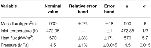
Table 1. Statistical parameters for the measured input variables.

Analysis Methodology

Brief Introduction on the Uncertainty Analysis Methodologies

The uncertainty of a simulation can be estimated by uncertainty propagation method (Badillo et al., 2013), the accuracy extrapolation method (D'Auria et al., 2012), and comparison method (Oberkampf et al., 1998), among which the uncertainty propagation method is the most mature and common used one and can be implemented easily. The input uncertainty can be propagated through the analysis code and then be transferred to the predicted results. With this method, samples representing PDFs of input parameters were used as the inputs of the code to obtain the PDFs of results. As for the samples, they can be obtained by the random sampling method or the deterministic sampling methods. The random sampling method is more reliable but needs numerous samples; while the deterministic one has not been fully validated and is far from mature (Bestion et al., 2016).

In the past few decades, most uncertainty analyses associated to system codes were performed based on the random sampling methods (Espinosa-Paredes et al., 2010), or the random methods with surrogate models, such as response surface method (Prošek et al., 2016) and artificial neural network (Secchi et al., 2008). Issues related to random sampling method have been investigated thoroughly, such as the determining of sample size (Wilks, 1942) or the improvements on the sampling methods (Helton and Davis, 2003; Iman, 2008). When it comes to the CFD applications, the deterministic methods with fewer sample requirements were employed to obtain the input parameters due to the increase of computational cost compared to the system code applications. Hessling (2013) proposed an efficient deterministic method for sampling. However, the accuracy and reliability of deterministic method in CFD applications were not fully validated and far from mature (Thiem and Schäfer, 2014). Thus, in this work, we employed the random sampling method to get the input parameters for uncertainty analysis in spite of the huge computational efforts. The LHS method, an efficient sampling methodology developed based on the traditional random sampling and domain decomposition technology (Helton and Davis, 2003), was used instead of the traditional Monte Carlo method to improve the sampling efficiency.

Implementation of the Uncertainty Analysis

The CFD simulation on subcooled boiling flow was carried out using the commercial code FLUENT. Eulerian–Eulerian two-fluid model along with the interphase actions and wall boiling models used in FLUENT has been validated in our previous work (Zhang et al., 2015c). Besides, the sensitivities of the turbulence model, the mesh size and the near wall turbulence treatment have been studied (Krepper and Rzehak, 2012; Zhang et al., 2015b). According to previous study on turbulence models (Zhang et al., 2015b), the subcooled boiling simulations were carried out with the Realizable k-ε turbulence model and Enhanced wall function based on the grid with near wall cell Y-plus ranging from 20.2 to 33.1. Besides, the inlet boundary was set at the location 10 times upstream of the test section inlet with a fully developed velocity profile to avoid the effects of inlet velocity profile, since there was a long inducer prior to the inlet of heated section to ensure a fully developed flow in the experiment (Bartolomei and Chanturiya, 1967). The geometry and boundary conditions of the computation domain are illustrated in Figure 1.

FIGURE 1

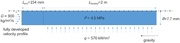
Figure 1. Geometry and boundary conditions.

The DAKOTA code (Adams et al., 2017), an uncertainty analysis code developed by the Sandia National Laboratory, was employed to generate the samples with LHS method, to drive the FLUENT code and to post-process the results. An interface was developed to allow the connection between DAKOTA and FLUENT codes by using Python script and the Internet Inter-ORB Protocol (IIOP) interface. The data flow chart is shown in Figure 2. A python subroutine is called by the DAKOTA code as an interface between DAKOTA code and the IIOP interface, which is an addon to allow the usage of FLUENT code as a server session. The physical properties of water may be effected by the input parameters, such as system pressure. Thus, a User-Defined Function (UDF) is compiled into standard FLUENT solver to call the IAPWS dynamics link library for liquid and vapor properties.

FIGURE 2

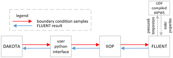
Figure 2. Data flow chart for the uncertainty analysis.

As mentioned above, the uncertainty propagation with random sampling method always needs numerous samples and runs to capture the statistical characteristics of inputs and outputs. Then the performance of the code could be evaluated. However, how many samples are enough from the view of statistics? Wilks presented an equation to correlate the confidence level, the coverage rate and the size of samples (Wilks, 1942), which has been extensively used in literature. Nevertheless, some other works increase the size of samples until the statistical parameters converge (Bestion et al., 2016). In our work, the Wilks's correlation under the condition of two-sided limits was employed to estimate the preliminary sample size for the inputs and then the sample size was increased until the value of expectation and standard deviation converge.

Results and Discussions

Multiple sets of output can be obtained in the uncertainty analysis with error propagation method. Three-dimensional variables should be analyzed to understand the statistical characteristics of the two-phase flow features. Six variables were chosen among the numerous data to present the averaged and local two-phase characteristics, including,

1) the pressure drop between inlet and outlet boundaries to quantify the flow resistance characteristics;

2) the averaged vapor fraction at the outlet, which is used to descript the total net vapor generation in the pipe;

3) the averaged wall temperature, which can present the heat transfer capacity at a boiling surface;

4) the location of net vapor generation, which is significant for the flow instability;

5) the ratio between maximum and averaged vapor volume fractions (VOFs) at outlet to represent the non-uniformity of the VOF distribution;

6) and the maximum wall VOF, which is associated with the boiling crisis according to the bubble crowding theory (Weisman and Pei, 1983).

Prior to the simulations, the preliminary size of samples was determined by using the Wilks's correlation (Wilks, 1942) and its variant (Pal and Makai, 2003). For problems with two-sided tolerance region, Wilks's correlations with first-order accuracy and high-order accuracy can be written as Equations (3) and (4), respectively.

$\begin{array}{ll}\beta =1-{\gamma }^N-N(1-\gamma ){\gamma }^{(N-1)}& (3)\end{array}$

$\begin{array}{ll}\beta ={\displaystyle \sum _{j=0}^{N-2n}}\left(\begin{array}{c}N\\ j\end{array}\right){\gamma }^j{(1-\gamma )}^{N-j}& (4)\end{array}$

where β, N, n, and γ are the confidence level, sample size, order of accuracy and coverage probability of the confidence interval, respectively. The sample size N can be obtained by solve the correlation with the requirement of 95/95% rule, that is, the coverage probability of confidence interval is no < 95% with a confidence level no < 95%. The minimum sample requirements for first, second and third order accuracy are 93, 153, and 208, respectively. Liu (2014) investigated the uncertainty of velocity profile predicted by a CFD code for forced convection in a cavity with Monte Carlo sample method and found that 153 samples can reach convergence results. However, as pointed out by Bestion et al. (2016) it may not reach the convergence values for the expectation and standard deviation when the samples size determined by this Wilks's equation was used. Thus, we increased the sample size until the statistical characteristics converged. The convergence history is shown in Figure 3. As can be seen, the convergence results can be obtained when the sample size is as large as 740, which is the sample size calculated by Wilks's equation with fourteenth order of accuracy.

FIGURE 3

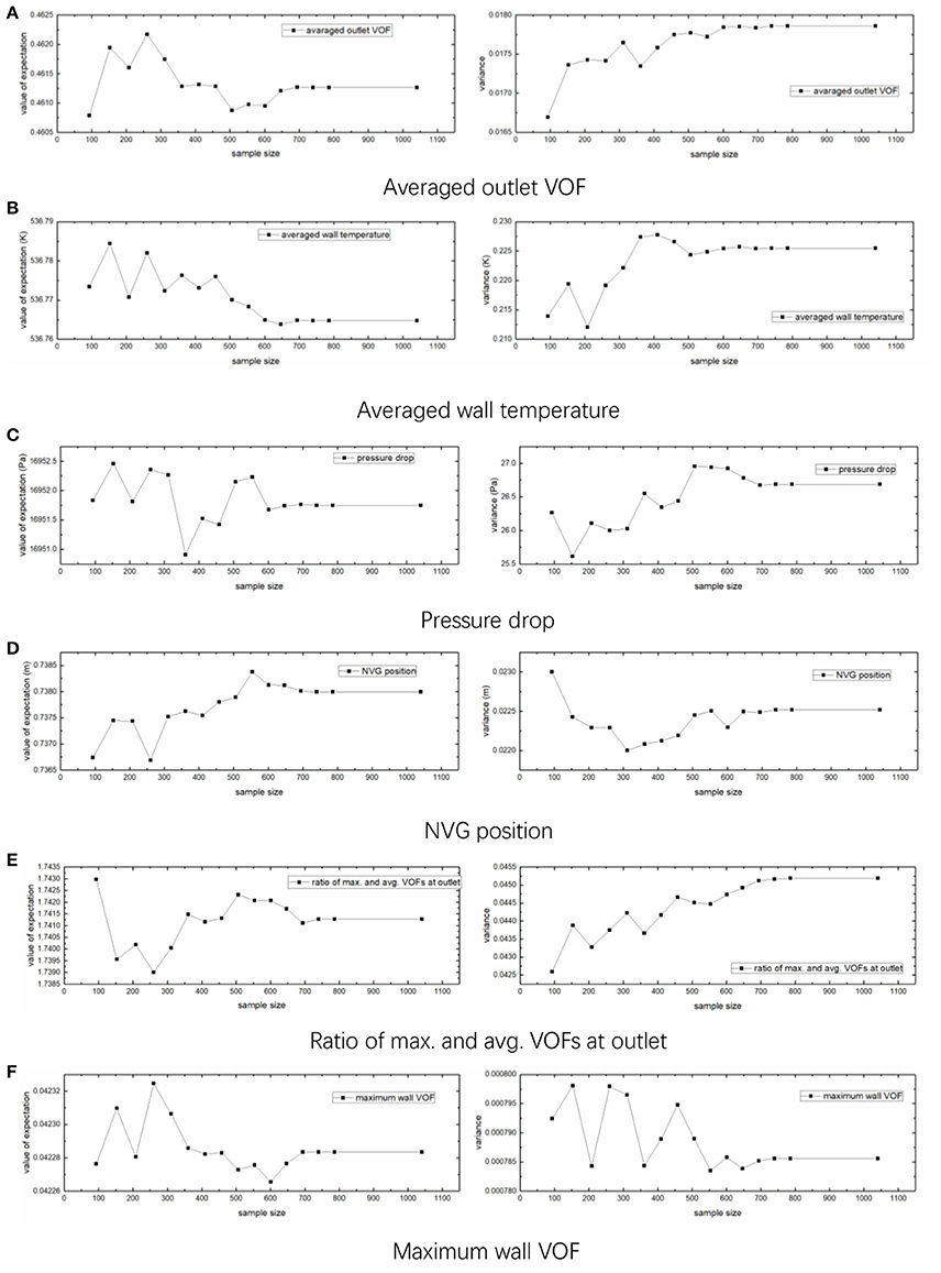
Figure 3. Convergence curve for expectation and standard deviation. (A) Averaged outlet VOF. (B) Averaged wall temperature. (C) Pressure drop. (D) NVG position. (E) Ratio of max. and avg. VOFs at outlet. (F) Maximum wall VOF.

After carrying out 740 runs of calculation, we can obtain the resultant two-phase parameters with consideration of the input uncertainty, including the averaged parameters and localized parameters as shown in Table 2. First of all, the statistical characteristics of the calculated vapor fraction, fluid temperature, and wall temperature were analyzed and compared with the experiment data (Bartolomei and Chanturiya, 1967; Wang et al., 2016)¹. The averaged value, 95% confidence interval and the +3σ interval are presented in Figure 4. It can be noted that the predicted cross-section averaged VOF and fluid temperature and their error bands agree quite well with the experiment data. However, there are slight deviations between the calculated and measured wall temperature, which might because the wall heat partition models used to simulate the boiling process at wall. Besides, the distribution of wall temperature is rather concentrated and its uncertainty is small. The effects of input uncertainties on the vapor fraction increase with the vapor fraction while wall temperature shows fewer impacts caused by the input uncertainty with increasing the vapor fraction.

TABLE 2

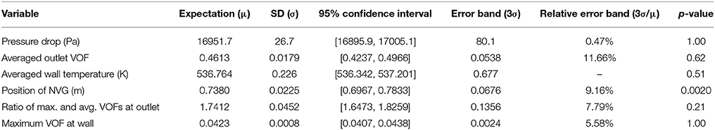
Table 2. Statistical characteristics for the outputs.

FIGURE 4

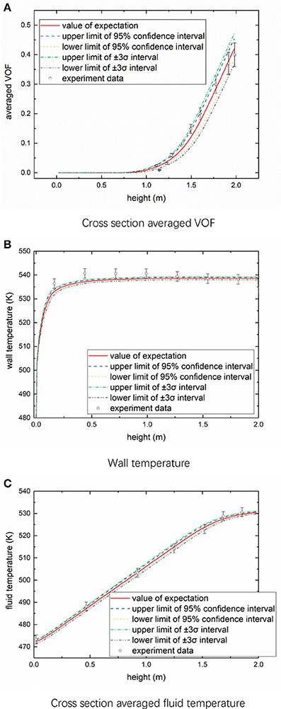
Figure 4. Value of expectation, 95% confidence interval and +3σ interval. (A) Cross section averaged VOF. (B) Wall temperature. (C) Cross section averaged fluid temperature.

Figure 5 presents the histograms of above mentioned six representative outputs. As can be seen, the statistical distributions of these parameters follow the rule of high probability density in the middle of the interval and low value at the two ends of the interval, which is consistent with the probability density of inputs. However, the distribution is diverse from the normal distribution to some degree. This means, the statistical characteristics of the inputs change during the propagation of uncertainty in the FLUENT code.

FIGURE 5

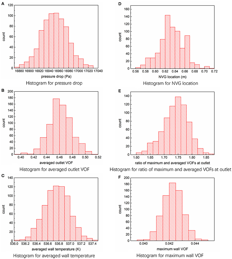
Figure 5. Histograms for output parameters. (A) Histogram for pressure drop. (B) Histogram for averaged outlet VOF. (C) Histogram for averaged wall temperature. (D) Histogram for NVG location. (E) Histogram for ratio of maximum and averaged VOFs at outlet. (F) Histogram for maximum wall VOF.

To quantify the PDF characteristics of these six variables, the statistical characteristics of these parameters were given in Figure 5, including expectations, standard deviations, 95% confidence interval, error bands, relative error bands, and the p-value for normality test. Here we also use the +3σ as the error band. As can be noted, the ranges of deviations for the outputs vary from each other. The uncertainties of the outlet VOF, NVG position, ratio of maximum and averaged VOFs at outlet and wall maximum VOF are much larger than the input uncertainties, while the uncertainties of the pressure drop and wall averaged temperature are less than the input uncertainties. That means, the outlet VOF, NVG position, ratio of maximum, and averaged VOFs at outlet and wall maximum VOF are much more sensitive to the input uncertainty than the pressure drop and wall averaged temperature under the calculated condition. Moreover, the p-values resulted from normal distribution test show that the pressure drop, averaged outlet VOF, averaged wall temperature, ratio of maximum and averaged VOFs at outlet and wall maximum VOF follow the normal distribution well while the position of NVG doesn't.

The scatter plots between the inputs and outputs are given in Figure 6 to illustrate the relationships between the boundary conditions and the interested parameters. As can be found, the mass flux has a significant linear effect on the pressure drop, that is, the pressure drop increases with mass flux linearly. The averaged outlet VOF, averaged wall temperature and maximum VOF at wall show slight decrease tendency with increasing mass flux. The NVG position and averaged outlet VOF increase with the mass flux, obviously. The temperature of fluid at inlet has dramatic impacts on the averaged outlet VOF, NVG position, and VOF ratio, while has little impacts on the pressure drop, averaged wall temperature and maximum wall temperature, which is because of the dependency of inlet enthalpy on the inlet temperature. The wall heat flux shows strong correlations with all the outputs except the pressure drop. The averaged outlet VOF, averaged wall temperature and maximum wall VOF increase with increasing the wall heat flux, while position of NVG and VOF ratio decrease. This is caused by the effects of wall heat flux on the nucleation process and the generation rate of vapor phase. Besides, the averaged wall temperature depends on the system pressure, due to the relationship between saturated temperature and system pressure.

FIGURE 6

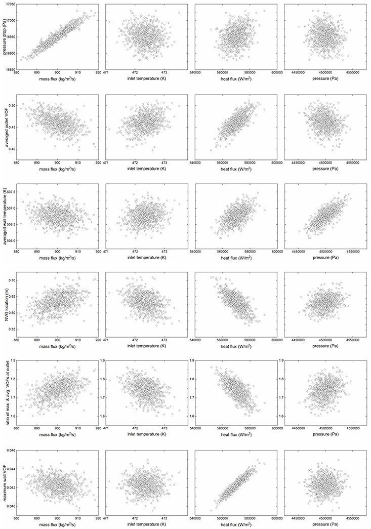
Figure 6. Scatter plots between the boundary conditions and outputs.

In the field of statistical analysis, covariance can be used to descript the dependency or correlation between two sets of samples. However, the values of covariance are associated with the absolute values of samples and cannot be used for the cross-comparison of the dependency between different sets of samples. The conception of correlation coefficient with values varying from zero to one was proposed to quantify the dependency of samples. The Pearson correlation coefficient was defined to quantify the linear dependency among samples, while the Spearman correlation coefficient was used to descript the more complicated dependency among samples, no matter linear or not (Hauke and Kossowski, 2011). Pearson and Spearman correlation coefficients are given in Figure 7 to quantify the relationship between boundary conditions and outputs. As can be seen, the effects of mass flux and heat flux on the subcooled boiling flow are much large than these of inlet temperature and system pressure. The absolute values of correlation coefficients between heat flux and most outputs, including averaged outlet VOF, averaged wall temperature, NVG position, and ratio of maximum and averaged VOFs at outlet, are larger than 0.5, which means there are strong dependencies among these variables. Besides, the Spearman and Pearson correlation coefficients are almost equal, which implies the dependencies between these parameters are linear. Besides, there is no dependency between the system pressure and pressure drop or maximum wall VOF since the absolute values of correlation coefficients are < 0.1.

FIGURE 7

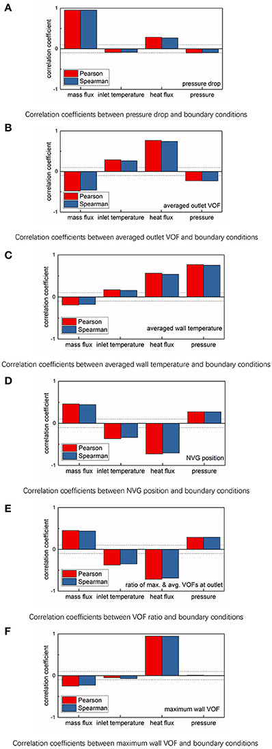
Figure 7. Correlation coefficients between boundary conditions and outputs. (A) Correlation coefficients between pressure drop and boundary conditions. (B) Correlation coefficients between averaged outlet VOF and boundary conditions. (C) Correlation coefficients between averaged wall temperature and boundary conditions. (D) Correlation coefficients between NVG position and boundary conditions. (E) Correlation coefficients between VOF ratio and boundary conditions. (F) Correlation coefficients between maximum wall VOF and boundary conditions.

Conclusions

In this work, the subcooled boiling flow was modeled by a CFD code (ANSYS FLUENT) with considering the uncertainty of boundary conditions. The uncertainty was analyzed by using the uncertainty propagation method with Latin Hypercube Sampling method. Seven hundred and forty sets of samples were employed as inputs to achieve the convergence results from the point of view of statistical analysis. Effects of uncertainties from boundary conditions on the two-phase characteristics were obtained. Following conclusions can be drawn from the results.

1) The sample size determined by Wilks's theorem with first order or second order of accuracy is not sufficient to get convergence results for complicated subcooled boiling from the view of statistics. Sample size should be increased until the statistical characteristics of the outputs converge. In this work, the sample size is as large as 740, which is the sample size calculated by Wilks's equation with fourteenth order of accuracy.

2) Uncertainties from heat flux and mass flux have more significant impacts on the subcooled boiling characteristics than these from inlet temperature and system pressure. Besides, the maximum wall VOF is affected by the heat flux uncertainty drastically.

Author Contributions

XZ and RZ: carried out the baseline case study on subcooled boiling, the sampling of boundary conditions, the results analysis; XL: wrote the python scripts for the uncertainty analysis and carried out the uncertainty analysis; TC: analyzed the results and wrote the paper.

Conflict of Interest Statement

The authors declare that the research was conducted in the absence of any commercial or financial relationships that could be construed as a potential conflict of interest.

Acknowledgments

This work is supported by National Natural Science Foundation of China (No. 11705035).

Footnotes

1. ^The experiment was performed by Bartolomei and Chanturiya (1967). However, this work only gave the error band for the input parameters, including the inlet temperature, heat flux, pressure, and mass flux. The error bands of for the fluid temperature, vapor fraction and wall temperature were not presented in this work. The error bands for these parameters were obtained from publication of Wang et al. (2016).

References

Adams, B., Ebeida, M., Eldred, M., Jakeman, J., Swiler, L., Bohnhoff, W., et al. (2017). Dakota, A Multilevel Parallel Object-Oriented Framework for Design Optimization, Parameter Estimation, Uncertainty Quantification, and Sensitivity Analysis: Version 6.6 Theory Manual. SAND2014-4253. Davis, CA: University of California.

Badillo, A., Kapulla, R., and Niceno, B. (2013). “Uncertainty quantification in CFD simulations of isokinetic turbulent mixing layers,” Proceedings of NURETH-15 (Pisa).

Badillo, A., Niceno, B., Fokken, J., and Kapulla, R. (2014). “Uncertainty quantification of the effect of random inputs on computational fluid dynamics simulations of the GEMIX experiment using metamodels,” Proceedings of CFD4NRS Conference (Zurich).

Bartolomei, G. G., and Chanturiya, V. M. (1967). Experimental study of true void fraction when boiling subcooled water in vertical tubes. Therm. Eng. 14, 123–128.

Google Scholar

Bestion, D., de Crécy, A., Camy, R., and Barthet, A. (2016). Review of Uncertainty Methods for CFD Application to Nuclear Reactor Thermal Hydraulics. NEA/CSNI/R(2016)4. OECD/NEA.

Chiasson, J. N. (2013). Introduction to Probability Theory and Stochastic Processes. Hoboken, NJ: John Wiley & Sons Inc.

Google Scholar

D'Auria, F., Camargo, C., and Mazzantini, O. (2012). The Best Estimate Plus Uncertainty (BEPU) approach in licensing of current nuclear reactors. Nucl. Eng. Des. 248, 317–328. doi: 10.1016/j.nucengdes.2012.04.002

CrossRef Full Text | Google Scholar

Espinosa-Paredes, G., Verma, S. P., Vázquez-Rodríguez, A., and Nuñez-Carrera, A. (2010). Mass flow rate sensitivity and uncertainty analysis in natural circulation boiling water reactor core from Monte Carlo simulations. Nucl. Eng. Des. 240, 1050–1062. doi: 10.1016/j.nucengdes.2010.01.012

CrossRef Full Text | Google Scholar

Hauke, J., and Kossowski, T. (2011). Comparison of values of Pearson's and Spearman's correlation coefficients on the same sets of data. Quaest. Geogr. 30, 87–93. doi: 10.2478/v10117-011-0021-1

CrossRef Full Text | Google Scholar

Helton, J. C., and Davis, F. J. (2003). Latin hypercube sampling and the propagation of uncertainty in analyses of complex systems. Reliab. Eng. Syst. Safety 81, 23–69. doi: 10.1016/S0951-8320(03)00058-9

CrossRef Full Text | Google Scholar

Hessling, J. P. (2013). Deterministic sampling for propagating model covariance. SIAM/ASA J. Uncertain. Quantif. 1, 297–318. doi: 10.1137/120899133

CrossRef Full Text | Google Scholar

Iman, R. L. (2008). “Latin hypercube sampling,” in Encyclopedia of Quantitative Risk Analysis and Assessment, eds E. L. Melnick and B. S. Everitt (Hoboken, NJ: John Wiley & Sons Inc.). doi: 10.1002/9780470061596.risk0299

CrossRef Full Text | Google Scholar

Knio, O., and Le Maitre, O. (2006). Uncertainty propagation in CFD using polynomial chaos decomposition. Fluid Dyn. Res. 38, 616–640. doi: 10.1016/j.fluiddyn.2005.12.003

CrossRef Full Text | Google Scholar

Krepper, E., and Rzehak, R. (2012). CFD Analysis of a void distribution benchmark of the NUPEC PSBT tests: model calibration and influence of turbulence modelling. Sci. Technol. Nucl. Instal. 2012:939561. doi: 10.1155/2012/939561

CrossRef Full Text | Google Scholar

Liu, Y. (2014). Investigation on Non-deterministic Methodologies and Application in CFD Simulation. Ph.D. thesis, North China Electric Power University, Beijing.

Oberkampf, W. L., Sindir, M., and Conlisk, A. (1998). Guide for the Verification and Validation of Computational Fluid Dynamics Simulations. Reston, VA: AIAA.

Pal, L., and Makai, M. (2003). Remarks on statistical aspects of safety analysis of complex systems. Reliab. Eng. Sys. Safety 80:217. arXiv preprint physics/0308086.

Prošek, A., Končar, B., and Leskovar, M. (2016). Uncertainty analysis of CFD benchmark case using optimal statistical estimator. Nucl. Eng. Des. 321, 132–143. doi: 10.1016/j.nucengdes.2016.12.008

CrossRef Full Text

Secchi, P., Zio, E., and Di Maio, F. (2008). Quantifying uncertainties in the estimation of safety parameters by using bootstrapped artificial neural networks. Ann. Nucl. Energy 35, 2338–2350. doi: 10.1016/j.anucene.2008.07.010

CrossRef Full Text | Google Scholar

Thiem, C., and Schäfer, M. (2014). “Acceleration of sampling methods for uncertainty quantification in computational fluid dynamics,” in Proceedings of the Ninth International Conference on Engineering Computational Technology (Naples: Civil-Comp Press).

Google Scholar

Wang, Z., Shaver, D. R., and Podowski, M. Z. (2016). On the modeling of wall heat flux partitioning in subcooled flow boiling. Trans. Am. Nucl. Soc. 114, 881–883.

Google Scholar

Weisman, J., and Pei, B. (1983). Prediction of critical heat flux in flow boiling at low qualities. Int. J. Heat Mass Transfer 26, 1463–1477. doi: 10.1016/S0017-9310(83)80047-7

CrossRef Full Text | Google Scholar

Wilks, S. S. (1942). Statistical prediction with special reference to the problem of tolerance limits. Ann. Math. Stat. 13, 400–409. doi: 10.1214/aoms/1177731537

CrossRef Full Text | Google Scholar

Zhang, R., Cong, T., Tian, W., Qiu, S., and Su, G. (2015a). CFD analysis on subcooled boiling phenomena in PWR coolant channel. Prog. Nucl. Energy 81, 254–263. doi: 10.1016/j.pnucene.2015.02.005

CrossRef Full Text | Google Scholar

Zhang, R., Cong, T., Tian, W., Qiu, S., and Su, G. (2015b). Effects of turbulence models on forced convection subcooled boiling in vertical pipe. Ann. Nucl. Energy 80, 293–302. doi: 10.1016/j.anucene.2015.01.039

CrossRef Full Text | Google Scholar

Zhang, R., Cong, T., Tian, W., Qiu, S., and Su, G. (2015c). Prediction of CHF in vertical heated tubes based on CFD methodology. Prog. Nucl. Energy 78, 196–200. doi: 10.1016/j.pnucene.2014.10.001

CrossRef Full Text | Google Scholar