Optimized Balance Between Electricity Load and Wind-Solar Energy Production

1. Introduction

Worldwide, energy systems are likely to become more dependent on weather due to the growing share of renewable power sources such as wind and solar (Wan and Parsons, 1993; Widén, 2011; Grams et al., 2017; Staffell and Pfenninger, 2017). Both energy sources are considered as “intermittent” due to their intrinsic variability. Wind power production exhibits variations on all timescales (Holttinen, 2005; Albadi and El-Saadany, 2010). In this respect, Van der Hoven (1957) identified three distinct peaks of wind speeds variability and their most important timescales: (i) the turbulent peak in the subsecond to minute range, (ii) the diurnal peak, driven by the heating and cooling of the earth surface, and (iii) the synoptic peak which depends on changing weather patterns with a scale of variation which ranges from days to weeks (Nikolakakis and Fthenakis, 2011; Coker et al., 2013; Grams et al., 2017). Annual and inter-annual (or decadal) variability represent important peaks as well (Sinden, 2007; Isyumov, 2012). Thus, the variability of wind power production might be classified into regular cycles (diurnal and seasonal/annual), and irregular cycles (synoptic, inter-annual). In contrast to wind speed, solar irradiation presents more defined annual and daily cycles (Coker et al., 2013). The observable irregular variations (synoptic and inter-annual) are related to the movement and persistence of clouds and to temperature gradients and drifts (Gueymard and Wilcox, 2009; Hoff and Perez, 2010; Mills, 2010; Kleissl et al., 2012). In addition, electricity load usually shows well-defined annual, daily, and weekly cycles (Wan, 2005; Coker et al., 2013) plus inter-annual and weekly variations (Wan, 2005; Wild et al., 2015) associated with economic activity and changing weather patterns.

For the reasons described above, the integration of these resources into a power grid may affect several stages of its operation and planning, such as grid frequency control (within the second to minute range), electricity load following operations (within the minutes to hours range), and the unit commitment scheduling (over the weekly timescale). It may increase the margin of spinning reserves to protect the system against sudden variations in electricity load or renewable power fluctuations and the need for flexibility in order to cope with higher ramping rates in energy production (Wan and Parsons, 1993; Smith et al., 2007; Nikolakakis and Fthenakis, 2011; Widén, 2011;Huber et al., 2014).

Besides the temporal variations described above, wind and solar resources also fluctuate geographically (Wan and Parsons, 1993). Studying these spatial variations of the wind and solar outputs is important for two reasons. Firstly, the aggregation of disperse intermittent power sources reduce their overall variability (Beyer et al., 1989; Wan, 2005; Kempton et al., 2010; Delucchi and Jacobson, 2011; Holttinen et al., 2011; Widén, 2011; Monforti et al., 2014). Secondly, it may help to optimize the complementarity between different renewable power sources and the system load (Wan and Parsons, 1993; Widén, 2011; Monforti et al., 2014; Grams et al., 2017).

The smoothing effect from geographical dispersion has been widely studied for wind power (Wan, 2005; Heide et al., 2010; Widén, 2011). It is well-known that a wider geographical distribution of wind farms reduce their overall variability (Milligan and Artig, 1999; Simonsen and Stevens, 2004; Fant et al., 2016). This smoothing effect is proportional to the size of the area under consideration (Archer and Jacobson, 2007), since the correlation between wind patterns decrease as the distance between sites increase (Wan, 2004; Sinden, 2007). In contrast, fewer studies have addressed the effect of the geographical dispersion of solar generation (Widén, 2011). Several studies show that there is also a smoothing effect on the aggregation of dispersed solar power units, but less pronounced than for wind power (Jewell, 1986; Mills, 2010; Delucchi and Jacobson, 2011; Widén, 2011).

Studying the complementary of different renewable sources (along with electricity load) is a complex matter. It is a different perspective from traditional optimization schemes that seek to improve the energy output of wind and solar sites (El-Shimy, 2010; Said et al., 2017). The aim, instead, is to consider all renewable facilities as a whole. As pointed out by Sterl et al. (2018), there are different criteria by which to plan an adequate use of renewable resources. Some studies focus on smoothing the renewable power output (Hoicka and Rowlands, 2011; Jerez et al., 2013; Schmidt et al., 2016; Gunturu and Hallgren, 2017; Miglietta et al., 2017), while other studies focus on shaping the renewable power output so that it meets the seasonal and/or daily electricity load curve (Heide et al., 2010; Coker et al., 2013; Becker et al., 2014). The managerial implications of these approaches might be different depending on the location and the timescale that is analyzed, since wind and solar generation, and electricity load timeseries show distinct temporal behaviors (Coker et al., 2013). For example, some authors claim that solar generation usually correlates better with electricity load than wind generation over the diurnal (Wan and Parsons, 1993; Nikolakakis and Fthenakis, 2011; Coker et al., 2013) and seasonal timescales (Wan and Parsons, 1993).

The correlations between wind generation and electricity load, on the contrary, are less certain and site-dependent. In this sense, Holttinen (2005) found different seasonal and daily average variations in wind power production over distinct regions in Europe; and Grams et al. (2017) suggested that deploying wind farms in the Balkans instead of the North Sea would reduce synoptic-scale fluctuations over Europe. Therefore, as mentioned above, the optimal solution is strongly region-dependent. Heide et al. (2010) proposed for Europe an optimal seasonal mix of 55% wind and 45% solar generation since wind correlates better with the seasonal electricity load curve than solar generation; and Coker et al. (2013) also found that wind generation in UK correlates better with the seasonal electricity load curve than solar generation. Widén (2011) and Monforti et al. (2014) studied the complementarity over different timescales of wind and solar generation over Sweden and Italy, respectively. They found negative distance independent correlations between solar and wind power over all timescales, but stronger for monthly averages. Becker et al. (2014) incorporates additional criteria to this analysis. They used three different approaches to optimize the wind and solar mix: minimizing the required storage capacity, minimizing system imbalance and levelized costs of renewable generation.

In this study we propose an optimization which reduces the variability of residual power, defined as the difference between electricity load and the solar and wind power output. We apply it for the optimization of future renewable power addition scenarios in Argentina. This country has an appreciable potential for wind and solar power generation (Hoogwijk et al., 2004; De Vries et al., 2007; Lu et al., 2009; Dupont et al., 2018). The share of wind and solar power is likely to increase in the incoming years. The country is committed to raise the share of renewables up to 12% for the year 2019, and up to 20% by the year 2025. Several tenders have been celebrated: 1470 MW of solar and 3020 MW of wind power were awarded. Besides the high quality of the wind and solar power resources, Argentina has the additional advantage of its wide geographical extension, which determines the existence of very distinct climatic regimes (Prohaska, 1976; Garreaud et al., 2009) (and, hence, distinct cloudiness and wind variability patterns) which should be considered when planning the deployment of wind and solar generation facilities. Hence, understanding the properties of local variations of these power sources is crucial for the development, optimization, and operation of the harvesting infrastructure.

2. Methodology

The methodology described below can be applied to any study in which wind and solar data is available at several geographically distributed energy production sites. Herein we dealt with the Argentinean sites described in Tables S2, S3, Appendix 2.

The methodology can be dissected in the following steps:

1. Collect site locations

2. Obtain wind speed and solar irradiation time series

3. Convert resources to power

4. Optimize balance between production and electricity load

Step 1 provides the location of every wind and solar site either installed or projected. We also obtained information about the technology used, for example tracking capabilities of solar panels.

Step 2 produces time series of the resources at each site. This can be achieved by using reanalysis data or by applying downscaling procedures (e.g., Martinez et al., 2013).

The last step before optimization comprises the conversion of the time series, from resources to electrical power production. For this step we used previously developed methods (Pfenninger and Staffell, 2016; Staffell and Pfenninger, 2016).

The final step is the numerical optimization of the total power production time series in relation to the electricity load. This optimization reduces the variance of the residual power, obtained by subtracting the total wind and solar power production from the electricity load. The optimization of the residual power was carried out in several scenarios relevant for the renewable energy development of the region under study. Each scenario portrays different levels of expansion of the total renewable power production capacity.

2.1. Collection of Sites

A total of 46 wind sites and 21 solar sites were used in this study. Site locations were extracted from Argentinean tenders GENREN, RENOVAR 1, RENOVAR 1.5, RENOVAR 2.0, and resolutions 108/11 and 202/16. A complete list of the sites and their characteristic is given in the Appendix (see Tables S2, S3). Their geographical location within the country are shown in Figure 1. The distribution of these sites span a great portion of the country where not only there are strong winds or high solar irradiance; but also have proven some degree of feasibility: proximity to the electric grid, accessibility, or reduced environmental impact.

FIGURE 1

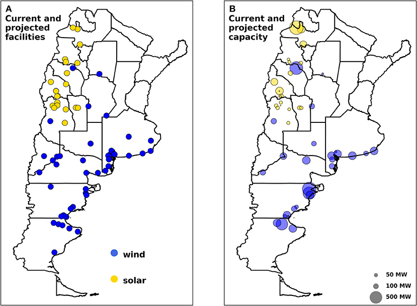
Figure 1. (A) Location of solar (in yellow) and wind (blue) sites. (B) Capacity projected at each site For details at each site see Tables S2, S3.

2.2. Resource Time Series for Each Site

For each site, we obtained wind speed data by performing WRF (Weather Research and Forecasting model) simulations fed with GFS (Global Forecast System) input data.

For solar resources we used irradiance data from the Modern Era Reanalysis for Research and Applications 2 (MERRA2) (National Aeronautics and Space Administration, 2016).

MERRA2 data set also provides a fairly good estimation of wind speeds, although this data failed to capture relevant temporal features present in several of the selected sites as we will show. We ascribe this to the locality of wind speed variations, which are well below the MERRA2 data set resolution (~50 km). We choose to implement WRF simulations for wind speed instead.

2.2.1. WRF Simulations

WRF is a state-of-the-art non-hydrostatic high resolution mesoscale model (Skamarock et al., 2005; Skamarock and Klemp, 2008). It was developed and maintained by several institutes including the National Center for Environmental Prediction (NCEP) and the National Center for Atmospheric Research (NCAR). To run a simulation using WRF the user needs to provide initial and boundary conditions on the geographical domain. The boundary conditions are time dependent, providing the inflow and outflows into the simulation domain. The initial and 6 h boundary conditions were taken from the GFS operational 0.5° × 0.5° resolution global analysis (Campana et al., 2005; Saha et al., 2014). These data was also used to nudge the simulation every 12 h, using default nudging settings.

In order to gain accuracy of the estimated wind velocity at 100 m height above the ground, we added an additional eta-levels to the simulation. These levels were inserted between each of the default 28 eta-levels in the namelist, rendering a final total of 55 eta-levels.

We found a good relation between results quality and computing time using grid resolutions set to 16 km for the main domain and 6 km for the nested domain.

For physics models and other settings we left default values. An overview of the model domain configuration and physics schemes used are shown in Table 1.

TABLE 1

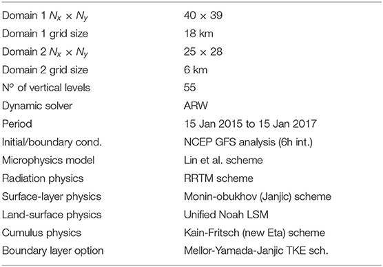
Table 1. Overview of WRF configuration for simulation of local wind time series.

2.3. Conversion to Power Production

A simulation of wind and solar power production encompassing a 2-year period was performed over all sites. The Virtual Wind Farm (VWF¹) model developed in Staffell and Green (2014) and Staffell and Pfenninger (2016) was used to simulate wind power production from wind speeds at 100 m height, using wind speeds based on WRF simulations. Once data was obtained, wind power outputs were computed using power curves of wind turbine generator according to the first criteria of the IEC standard classes (International Electrotechnical Commission, 2005), which we summarize in the Appendix.

Before convolving wind speeds with their corresponding power curve, power curves values were smoothed using a Gaussian filter, as proposed in the VWFM method.

For power production based on solar irradiance, we used the The Global Solar Energy Estimator (GSEE²), developed by Pfenninger and Staffell (2016). This method calculates direct and diffuse irradiances using the short wave ground-level global irradiance variable SWGDN and top of atmosphere irradiance SWTDN from the closest MERRA2 grid point. The model then calculates the irradiance on the plane of the solar panels, whether panels are fixed or have tracking capabilities. Skin temperature variable is also used by the model to finally adjust the power output obtained through temperature-efficiency curves.

2.4. Optimization of Balance Between Renewables Generation and Electricity Load

In this section we propose a method to find the best distribution of additional capacity (capacity added after current projects) that minimizes the variance of residual power.

Let a_i be current tendered and working projects capacities (depicted in Tables S2, S3), and v_i the hourly capacity factor of the ith site. Then the hourly power series of current projects is

$\begin{array}{ll}{P}_{\text{curr}}(t)={\displaystyle \sum _{i=1}^N}{a}_i{v}_i(t),& (1)\end{array}$

where N is the number of all sites.

If b_i is the additional power capacity to the ith site and w_i(t) is the hourly capacity factor of that site, then the hourly total additional power series reads

$\begin{array}{ll}{P}_{\text{addit}}(t)={\displaystyle \sum _{i=1}^N}{b}_i{w}_i(t),& (2)\end{array}$

The coefficients obey a_i, b_i ≥ 0. Additionally, if P_load(t) is the electricity load, then the residual power (considering both current and additional projects) is defined as

$\begin{array}{ll}{P}_{\text{resid}}(t)=P_{\text{load}}(t)-P_{\text{curr}}(t)-P_{\text{addit}}(t),& (3)\end{array}$

which is the remaining power to be supplied after the contribution from wind and solar facilities.

The optimization problem can be stated as follows: given a total energy contribution of additional projects

$\begin{array}{ll}{E}_{\text{add}}={\displaystyle \int }{P}_{\text{addit}}(t)\text{d}t={\displaystyle \sum _{i=1}^N}{b}_i{\displaystyle \int }{w}_i(t)\text{d}t=T{\displaystyle \sum _{i=1}^N}{b}_i\overline{w_i},& (4)\end{array}$

find the distribution of additional capacity over sites b_i that minimizes the variance of residual power var(P_resid). In the equation above, T is the total time span of the signals and $\overline{w_i}$ is their temporal average. The formal details of this optimization are given in the Appendix 3.

Instead of fixing the total energy, one could have constrained the sum of additional capacity $\sum _i{b}_i$, but in this case sites with lower average capacity would prevail, as they have less impact on residual power dispersion. Fixing E_add eliminates this possibility.

Summarizing, the optimization problem reduces to the following statement; given a prescribed additional energy E_add (Equation 4), find the additional capacity distribution at each site b_i from Equation (2) that minimizes the dispersion of P_resid(t) in Equation (3).

3. Results

3.1. Wind and Solar Power Production Simulations

Geographical location of all collected 46 wind and 21 solar parks within the country are shown in Figure 1.

Once wind and solar power time series were obtained for all sites respectively, we proceeded to study the hypothetical incidence of planned projects on the 2015/16 electricity load.

Renewable capacity either installed or projected results in a total of 2458 MW for wind sites and 924.5 MW for solar sites, an overall of 3382 MW. The resulting total output of the current projected and existing facilities is shown in Figure 2. These results show that, if all current and projected facilities would have operated during 2015-2016, they would have yielded a total capacity factor of 47%; 54% for wind parks and 28% from solar parks, delivering an average of 13.9 GW h per year.

FIGURE 2

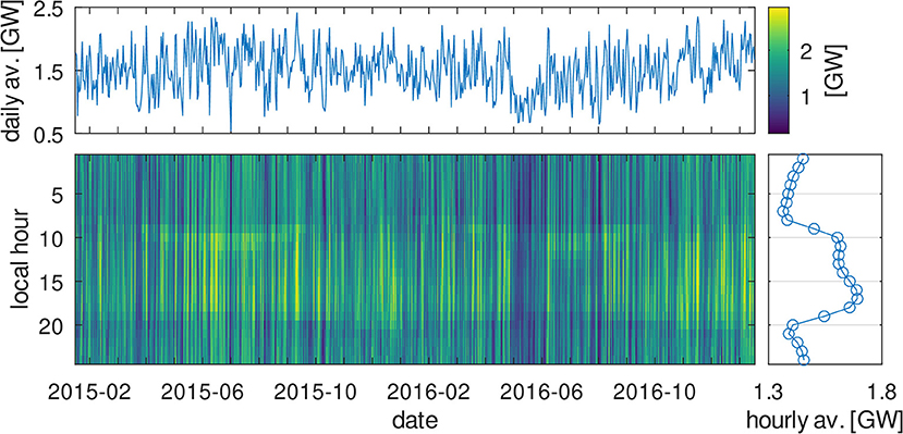
Figure 2. Power series from years 2015 and 2016 of overall 3382.5 MW wind and solar facilities, as listed in Tables S2, S3. 2458 MW correspond to wind facilities while 924.5 MW correspond to solar facilities. The overall capacity factor obtained is 47%, with a coefficient of variation of 29%. Solar site's mean capacity factor is 28% (coefficient of variation 110%) and wind site's mean capacity factor is 54% (coefficient of variation 37%). Current and projected capacity of renewables would have covered 10% of the overall electricity load.

We also analyzed the compatibility between renewables and electricity load through the years 2015 and 2016. Figure 3 shows the electricity load curve for this period, provided by the national grid administrator (CAMMESA). As expected, electricity load shows well-defined annual, weekly and daily cycles, with a dispersion equal to σ_load = 2352 MW. Subtracting the renewable power production during this period yields a residual power time series with dispersion σ_{load−renewables} = 2383 MW, slightly above dispersion from electricity load. We noted that hourly peaks of electricity load would have been reduced from 23.2 to 21.3 GW; while the hourly valleys of electricity load would have been reduced from 9.6 to 7.6 GW.

FIGURE 3

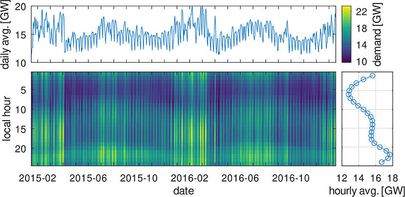
Figure 3. Electricity load from 2015 to 2016, provided by the national grid administrator. Average electricity load is 15.1 GW, with peaks of 23 GW, and valleys of 9.6 GW.

3.2. Optimally Balanced Additional Renewable Capacity

We analyze how to add further wind and solar power capacity, while minimizing intermittence effects. As mentioned in section 2.4, we have chosen our objective function to be the variance of the residual power, defined as electricity load minus wind and solar renewables generation (see Equation 3).

The optimized distribution of renewable capacity additions is depicted in Figure 4. Dashed lines are obtained by rescaling the currently installed and projected capacity, i.e., rescaling capacity while keeping their current distribution. Solid lines show the result of optimizing the added capacity beyond projected capacity. That is to say, for every value in the solid curve greater than projected capacity (a share above ~10% of 2015/2016 electricity load) the additional capacity distribution is optimized as explained in section 2.4. Note that for high shares (>30%), the dispersion increases almost linearly with increasing share.

FIGURE 4

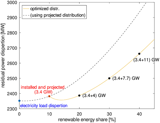
Figure 4. Plot of the dispersion σ of residual power (electricity load minus renewables) in different scenarios: (dashed line) capacity with constant distribution as currently installed and projected; (solid line) future additional capacity optimized to diminish σ at each value.

We propose three different scenarios of optimized additional capacity: (i) increasing renewables share to 20%, (ii) 30%, and (iii) 40%, and analyze the distribution in each one of them. The results are shown in Figure 5.

FIGURE 5

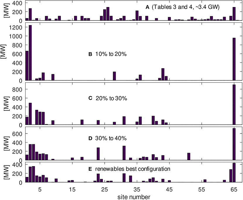
Figure 5. Power capacity distribution of sites. (A) Installed and project capacity detailed in Tables S2, S3 (3.4 GW); (B) 4.0 GW added capacity to reach 20% in energy share; (C) 3.7 GW added capacity to reach 30% share; (D) 3.45 GW to reach 40%; (E) renewables configuration with least dispersion, rescaled to achieve 10% of electricity load during 2015–2016 (3.4 GW).

Figure 5A shows the distribution of installed and current tendered capacity, described in Tables S2, S3. As mentioned above, the coefficient of variation of this distribution is 0.30 and the capacity factor is 0.44.

Figure 5B shows the distribution of 4.0 GW additional capacity that increases the share of wind and solar generation in another 10% while minimizing dispersion. Capacity differs from case to case, as also does the overall capacity factor in each of the distributions. Surprisingly we see that wind sites Arauco (#1) and Sosneado (#2) together with Cachaurí solar site (#65) receive more than 80% of the capacity. This can be explained by the hourly correlation between sites and electricity load (Figure 6), where we see that these are the sites most positively correlated with electricity load. The coefficient of variation of this distribution is 0.39 and the capacity factor is 0.37.

FIGURE 6

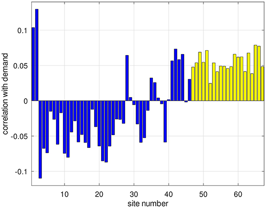
Figure 6. Hourly correlation between electricity load and capacity factor time series (blue bars for wind sites; yellow bars for solar sites). For site reference see Tables S2, S3.

Figure 5C shows the distribution of additional 3.45 GW capacity necessary to increase renewables from 20 to 30% in energy share. Here solar contribution at Caucharí site (#65) still prevails, although sites Arauco and Sosneado are diminished when compared to the previous scenario. The coefficient of variation of this distribution is 0.30 and the capacity factor is 0.41.

Figure 5D shows the last case, where share is increased from 30 to 40% with 3.4 GW additional capacity. The optimization in this upgrade focuses mainly in compensating variability between renewables, as can be seen if compared with Figure 5E. This is linked to the almost linear increase of dispersion observed in Figure 4 in regions of high share. The coefficient of variation of this distribution is 0.23, slightly above the lowest possible value obtained by mixing renewables time series. The resulting capacity factor is 0.45.

Finally, in order to contrast with the abovementioned cases, we performed a different optimization. The purpose of this optimization is to reduce variability of the output of wind and solar facilities (and not the residual load, as in the previous cases). This means that renewables would compensate among themselves. Figure 5E shows this distribution, scaled up to reach 10% of electricity load energy. The coefficient of variation of this distribution is 0.23, and the resulting capacity factor is 0.45. These values coincide with those of Figure 5D, however the allocation of capacity is not the same.

Summing up, when adding further capacity to increase energy share from 10 to 20%, optimization focuses in wind sites Arauco (#1) and Sosneado (#2) together with solar site Caucharí (#65) to counteract the variability of electricity load. The next additional 10% is a transition zone, where optimization starts compensating renewables inherent variability. In other words, electricity load admits up to ≈20% of renewable energy supply without increasing its variability. This relation can be further explored looking at the correlation between electricity load and each of the renewables time series, as shown in Figure 6. We see that electricity load positively correlates with solar outputs, but correlation with wind sites shows different behaviors. More than half of the wind sites anticorrelate with electricity load, particularly is the case of wind site #3 “El Jume” and also site #4 “Achiras.” These parks prevail when optimizing renewables between themselves, as we see in Figure 5E. The most positively correlated wind locations are sites #2 “Parque Arauco,” #1 “El Sosneado,” and #28 “Gastre,” located in center of Chubut province.

In Figure 7 we plot the daily averages of electricity load, positively correlated wind sites #1 and #2, and the anticorrelated wind site #3 All sites exhibit strong daily variations: in “Parque Arauco” and “El Sosneado” locations late afternoon winds prevail, while in “El Jume” wind blows mainly in night hours.

FIGURE 7

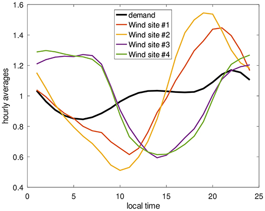
Figure 7. Hourly averages of electricity load of wind sites #1 and #2 (Sosneado and Arauco), #3 and #4 (El jume and Achiras) and electricity load. The resemblance between renewables time series and electricity load is reflected in their correlation, as shown in Figure 6.

Further information can be obtained from the histograms of the four residual power situations studied (Figure 8). Addition of renewable capacity smoothens the shape of the histograms and shifts them to the left, while widening is not visible. Situations with negative residual power are seen only in the last case, where renewables share supplies 40% of electricity load energy. In this case we see negative residual power with only ≈ 0.3% of occurrences, a total of 57 h through the 2015-2016 period.

FIGURE 8

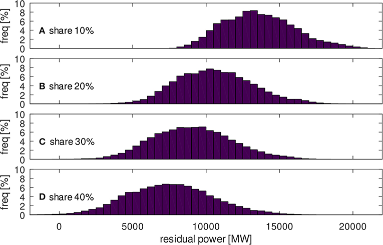
Figure 8. Histograms of residual power for the 2015–2016 electricity load scenario. (A) Assuming current installed and projected capacity; (B) 20% of renewables contribution to electricity load in energy terms; (C) 30%; (D) 40%. Bin width is 500 MW.

4. Discussion

In this article we analyzed the variability of wind and solar resources along with their compatibility with electricity load in Argentina, focusing on current facilities and projects under construction or awarded in recent tenders.

Wind and solar power simulations during the years 2015 and 2016, based on WRF simulations and MERRA2 data respectively yielded, for the current distribution of existing and tendered facilities, a capacity factor of 54% for wind parks and 28% for solar parks, resulting in an overall capacity factor of 47%. These facilities would have covered 10% of the overall electricity load in that period. Residual power (that is electricity load minus renewables) would have slightly increased its dispersion (2383 MW) if compared with the raw dispersion of electricity load (2352 MW), showing good compatibility with current installed and projected distribution. Hourly peaks of residual power would have been reduced from 23.2 to 21.3 GW; and hourly valleys from 9.6 to 7.6 GW.

An optimization of the distribution of wind and solar facilities aimed to diminish dispersion of the residual demand was performed for three scenarios of capacity additions: (i) from 10% of electricity load energy (installed and projected capacity) to 20%, (ii) from 20 to 30%, and (iii) from 30 to 40%. From this analysis we found that, focusing on dispersion only, the penetration of wind and solar facilities may double tendered capacity, while keeping dispersion almost constant. In this process the wind sites that most positively correlate with electricity load (“Parque Arauco” and “Sosneado”), together with Caucharí solar site, have the most important role in compensating electricity load variability.

The optimal distribution of further increasing renewables beyond ≈ 40% focuses on diminishing inherent renewables variability. In this distribution, locations where night winds are present such as sites #3 “El Jume” and #4 “Achiras” play an important role, as they compensate renewables that show higher availability during the day.

Results show also that curtailment events would not be frequent if solar and wind capacity is increased in an optimized scheme at least up to 40% of the share.

5. Conclusion

This work provided insights into the variability of wind and solar power and its compatibility with the electricity load. Many sites are left without capacity in the described scenarios. Certainly there are other aspects that may contradict these results, such as transport constraints, smoothness of high frequency variability or robustness of the grid. In future studies we will try to group renewables by similar characteristics, and also try other criteria of optimization. Focusing on the variance of residual demand is perhaps the simplest way to characterize intermittence, but there are many other aspects that would be more convenient to optimize, such as a studying the ramp plot of hourly variation or perhaps the behavior or the grid at certain locations. This work is a first approach to present the problem and characterize intermittence in the region, we hope to analyze more realistic intermittence function costs in the future.

Data Availability Statement

The datasets generated for this study (except those with electrical load and site measurements time series provided by CAMMESA) can be found in the Open Science Foundation repository https://doi.org/10.17605/OSF.IO/4XF35. For more information please write to the corresponding author.

Author Contributions

TG, JC, and EB contributed conception and design of the study. TG, JC, and AS performed the statistical analysis. EB wrote the first draft of the manuscript. TG, JC and EB wrote sections of the manuscript. All authors contributed to manuscript revision, read, and approved the submitted version.

Funding

This work has been supported by (1) Agencia Nacional de Promoción Científica y Tecnológica, (2) Universidad Nacional de Río Negro, (3) Swiss Federal Institute of Aquatic Science and Technology, and (4) Eawag Discretionary Funds (grant no.: 5221.00492.011.05, project: DF2017/EMUmore).

Conflict of Interest

The authors declare that the research was conducted in the absence of any commercial or financial relationships that could be construed as a potential conflict of interest.

Acknowledgments

The authors would like to thank Jorge Siryi and Joaquin Beitia of the national grid administrator: Compañía Administradora del Mercado Mayorista Eléctrico de Argentina (CAMMESA), who encouraged this research and provided electricity load and power production data.

Supplementary Material

The Supplementary Material for this article can be found online at: https://www.frontiersin.org/articles/10.3389/fenrg.2020.00016/full#supplementary-material

Footnotes

1. ^https://github.com/renewables-ninja/vwf

2. ^https://github.com/renewables-ninja/gsee

References

Albadi, M., and El-Saadany, E. (2010). Overview of wind power intermittency impacts on power systems. Electr. Power Syst. Res. 80, 627–632. doi: 10.1016/j.epsr.2009.10.035

CrossRef Full Text | Google Scholar

Archer, C. L., and Jacobson, M. Z. (2007). Supplying baseload power and reducing transmission requirements by interconnecting wind farms. J. Appl. Meteorol. Climatol. 46, 1701–1717. doi: 10.1175/2007JAMC1538.1

CrossRef Full Text | Google Scholar

Becker, S., Frew, B. A., Andresen, G. B., Zeyer, T., Schramm, S., Greiner, M., et al. (2014). Features of a fully renewable us electricity system: optimized mixes of wind and solar pv and transmission grid extensions. Energy 72, 443–458. doi: 10.1016/j.energy.2014.05.067

CrossRef Full Text | Google Scholar

Beyer, H., Luther, J., and Steinberger-Willms, R. (1989). “Power fluctuations from geographically diverse, grid coupled wind energy conversion systems,” in European Wind Energy Conference Proceedings (Birmingham), 306–310.

Google Scholar

Campana, K., Caplan, P., and Alpert, J. (2005). Technical Procedures Bulletin for the T382 Global Forecast System. Available online at: https://www.emc.ncep.noaa.gov/gc_wmb/Documentation/TPBoct05/T382.TPB.FINAL.htm

Google Scholar

Coker, P., Barlow, J., Cockerill, T., and Shipworth, D. (2013). Measuring significant variability characteristics: an assessment of three UK renewables. Renew. Energy 53, 111–120. doi: 10.1016/j.renene.2012.11.013

CrossRef Full Text | Google Scholar

De Vries, B. J., Van Vuuren, D. P., and Hoogwijk, M. M. (2007). Renewable energy sources: their global potential for the first-half of the 21st century at a global level: an integrated approach. Energy Policy 35, 2590–2610. doi: 10.1016/j.enpol.2006.09.002

CrossRef Full Text | Google Scholar

Delucchi, M. A., and Jacobson, M. Z. (2011). Providing all global energy with wind, water, and solar power, part II: reliability, system and transmission costs, and policies. Energy Policy 39, 1170–1190. doi: 10.1016/j.enpol.2010.11.045

CrossRef Full Text | Google Scholar

Dupont, E., Koppelaar, R., and Jeanmart, H. (2018). Global available wind energy with physical and energy return on investment constraints. Appl. Energy 209, 322–338. doi: 10.1016/j.apenergy.2017.09.085

CrossRef Full Text | Google Scholar

El-Shimy, M. (2010). Optimal site matching of wind turbine generator: case study of the Gulf of Suez Region in Egypt. Renew. Energy 35, 1870–1878. doi: 10.1016/j.renene.2009.12.013

CrossRef Full Text | Google Scholar

Fant, C., Gunturu, B., and Schlosser, A. (2016). Characterizing wind power resource reliability in Southern Africa. Appl. Energy 161, 565–573. doi: 10.1016/j.apenergy.2015.08.069

CrossRef Full Text | Google Scholar

Gambetta, P., and Doña, V. M. (2011). “Planta solar fotovoltaica san juan 1: Descripción de se diseño y detalles de operación,” in Cuarto Congreso Nacional — Tercer Congreso Iberoamericano Hidrógeno y Fuentes Sustentables de Energía — HYFUSEN 2011 (Bariloche).

Google Scholar

Garreaud, R. D., Vuille, M., Compagnucci, R., and Marengo, J. (2009). Present-day south american climate. Palaeogeogr. Palaeoclimatol. Palaeoecol. 281, 180–195. doi: 10.1016/j.palaeo.2007.10.032

CrossRef Full Text | Google Scholar

Grams, C. M., Beerli, R., Pfenninger, S., Staffell, I., and Wernli, H. (2017). Balancing Europe's wind-power output through spatial deployment informed by weather regimes. Nat. Clim. Change 7:557. doi: 10.1038/nclimate3338

PubMed Abstract | CrossRef Full Text | Google Scholar

Gueymard, C. A., and Wilcox, S. M. (2009). “Spatial and temporal variability in the solar resource: assessing the value of short-term measurements at potential solar power plant sites,” in Solar 2009 ASES Conf (Buffalo, NY).

Google Scholar

Gunturu, U. B., and Hallgren, W. (2017). Asynchrony of wind and hydropower resources in Australia. Sci. Rep. 7:8818. doi: 10.1038/s41598-017-08981-0

PubMed Abstract | CrossRef Full Text | Google Scholar

Heide, D., Von Bremen, L., Greiner, M., Hoffmann, C., Speckmann, M., and Bofinger, S. (2010). Seasonal optimal mix of wind and solar power in a future, highly renewable Europe. Renew. Energy 35, 2483–2489. doi: 10.1016/j.renene.2010.03.012

CrossRef Full Text | Google Scholar

Hoff, T. E., and Perez, R. (2010). Quantifying pv power output variability. Solar Energy 84, 1782–1793. doi: 10.1016/j.solener.2010.07.003

CrossRef Full Text | Google Scholar

Hoicka, C. E., and Rowlands, I. H. (2011). Solar and wind resource complementarity: advancing options for renewable electricity integration in Ontario, Canada. Renew. Energy 36, 97–107. doi: 10.1016/j.renene.2010.06.004

CrossRef Full Text | Google Scholar

Holttinen, H. (2005). Hourly wind power variations in the nordic countries. Wind Energy 8, 173–195. doi: 10.1002/we.144

CrossRef Full Text | Google Scholar

Holttinen, H., Meibom, P., Orths, A., Lange, B., O'Malley, M., Tande, J. O., et al. (2011). Impacts of large amounts of wind power on design and operation of power systems, results of iea collaboration. Wind Energy 14, 179–192. doi: 10.1002/we.410

CrossRef Full Text | Google Scholar

Hoogwijk, M., de Vries, B., and Turkenburg, W. (2004). Assessment of the global and regional geographical, technical and economic potential of onshore wind energy. Energy Econ. 26, 889–919. doi: 10.1016/j.eneco.2004.04.016

CrossRef Full Text | Google Scholar

Huber, M., Dimkova, D., and Hamacher, T. (2014). Integration of wind and solar power in Europe: assessment of flexibility requirements. Energy 69, 236–246. doi: 10.1016/j.energy.2014.02.109

CrossRef Full Text | Google Scholar

International Electrotechnical Commission (2005). International Standard iec 61400-1. Wind turbine generator systems-part, 1.

Google Scholar

Isyumov, N. (2012). Alan g. davenport's mark on wind engineering. J. Wind Eng. Indus. Aerodynam. 104, 12–24. doi: 10.1016/j.jweia.2012.02.007

CrossRef Full Text | Google Scholar

Jerez, S., Trigo, R., Sarsa, A., Lorente-Plazas, R., Pozo-Vázquez, D., and Montávez, J. (2013). Spatio-temporal complementarity between solar and wind power in the Iberian Peninsula. Energy Proc. 40, 48–57. doi: 10.1016/j.egypro.2013.08.007

CrossRef Full Text | Google Scholar

Jewell, W. T. (1986). Effects of Moving Cloud Shadows on Electric Utilities With Dispersed Solar Photovoltaic Generation. Technical report, Oklahoma State University, Stillwater, OK, United States.

Google Scholar

Kempton, W., Pimenta, F. M., Veron, D. E., and Colle, B. A. (2010). Electric power from offshore wind via synoptic-scale interconnection. Proc. Natl. Acad. Sci. U.S.A. 107, 7240–7245. doi: 10.1073/pnas.0909075107

PubMed Abstract | CrossRef Full Text | Google Scholar

Kleissl, J., Lave, M., Jamaly, M., and Bosch, J.-L. (2012). “Aggregate solar variability,” in Power and Energy Society General Meeting, 2012 IEEE (San Diego, CA: IEEE), 1–3.

Google Scholar

Lu, X., McElroy, M. B., and Kiviluoma, J. (2009). Global potential for wind-generated electricity. Proc. Natl. Acad. Sci. U.S.A. 106, 10933–10938. doi: 10.1073/pnas.0904101106

PubMed Abstract | CrossRef Full Text | Google Scholar

Martinez, Y., Yu, W., and Lin, H. (2013). A new statistical–dynamical downscaling procedure based on EOF analysis for regional time series generation. J. Appl. Meteorol. Climatol. 52, 935–952. doi: 10.1175/JAMC-D-11-065.1

CrossRef Full Text | Google Scholar

Miglietta, M. M., Huld, T., and Monforti-Ferrario, F. (2017). Local complementarity of wind and solar energy resources over Europe: an assessment study from a meteorological perspective. J. Appl. Meteorol. Climatol. 56, 217–234. doi: 10.1175/JAMC-D-16-0031.1

CrossRef Full Text | Google Scholar

Milligan, M. R., and Artig, R. (1999). Choosing Wind Power Plant Locations and Sizes Based on Electric Reliability Measures Using Multiple-Year Wind Speed Measurements. Technical report, National Renewable Energy Lab., Golden, CO, United States.

Google Scholar

Mills, A. (2010). Implications of Wide-Area Geographic Diversity for Short-Term Variability of Solar Power. Lawrence Berkeley National Laboratory.

Google Scholar

Monforti, F., Huld, T., Bódis, K., Vitali, L., D'isidoro, M., and Lacal-Arántegui, R. (2014). Assessing complementarity of wind and solar resources for energy production in Italy. A monte carlo approach. Renew. Energy 63, 576–586. doi: 10.1016/j.renene.2013.10.028

CrossRef Full Text | Google Scholar

National Aeronautics and Space Administration (2016). Available online at: https://gmao.gsfc.nasa.gov/reanalysis/MERRA-2/

Google Scholar

Nikolakakis, T., and Fthenakis, V. (2011). The optimum mix of electricity from wind-and solar-sources in conventional power systems: evaluating the case for New York state. Energy Policy 39, 6972–6980. doi: 10.1016/j.enpol.2011.05.052

CrossRef Full Text | Google Scholar

Pfenninger, S., and Staffell, I. (2016). Long-term patterns of European pv output using 30 years of validated hourly reanalysis and satellite data. Energy 114, 1251–1265. doi: 10.1016/j.energy.2016.08.060

CrossRef Full Text | Google Scholar

Prohaska, F. (1976). The climate of Argentina, paraguay and uruguay. Clim. Central South Am. 12, 13–112.

Google Scholar

Rhodes, B. C. (2011). Pyephem: Astronomical Ephemeris for Python. Astrophysics Source Code Library.

Google Scholar

Saha, S., Moorthi, S., Wu, X., Wang, J., Nadiga, S., Tripp, P., et al. (2014). The NCEP climate forecast system version 2. J. Clim. 27, 2185–2208. doi: 10.1175/JCLI-D-12-00823.1

CrossRef Full Text | Google Scholar

Said, M., El-Shimy, M., and Abdelraheem, M. (2017). Improved framework for techno-economical optimization of wind energy production. Sustain. Energy Technol. Assess. 23, 57–72. doi: 10.1016/j.seta.2017.09.002

CrossRef Full Text | Google Scholar

Schmidt, J., Cancella, R., and Junior, A. O. P. (2016). The effect of windpower on long-term variability of combined hydro-wind resources: the case of Brazil. Renew. Sustain. Energy Rev. 55, 131–141. doi: 10.1016/j.rser.2015.10.159

CrossRef Full Text | Google Scholar

Simonsen, T. K., and Stevens, B. G. (2004). “Regional wind energy analysis for the Central United States,” in Proc Global Wind Power (Grand Fork, ND), 16.

Google Scholar

Sinden, G. (2007). Characteristics of the UK wind resource: long-term patterns and relationship to electricity demand. Energy Policy 35, 112–127. doi: 10.1016/j.enpol.2005.10.003

CrossRef Full Text | Google Scholar

Skamarock, W. C., and Klemp, J. B. (2008). A time-split nonhydrostatic atmospheric model for weather research and forecasting applications. J. Comput. Phys. 227, 3465–3485. doi: 10.1016/j.jcp.2007.01.037

CrossRef Full Text | Google Scholar

Skamarock, W. C., Klemp, J. B., Dudhia, J., Gill, D. O., Barker, D. M., Wang, W., et al. (2005). A Description of the Advanced Research wrf version 2. Technical report, National Center For Atmospheric Research Boulder Co Mesoscale and Microscale Meteorology Div.

Google Scholar

Smith, J. C., Milligan, M. R., DeMeo, E. A., and Parsons, B. (2007). Utility wind integration and operating impact state of the art. IEEE Trans. Power Syst. 22, 900–908. doi: 10.2172/1218416

CrossRef Full Text | Google Scholar

Staffell, I., and Green, R. (2014). How does wind farm performance decline with age? Renew. Energy 66, 775–786. doi: 10.1016/j.renene.2013.10.041

CrossRef Full Text | Google Scholar

Staffell, I., and Pfenninger, S. (2016). Using bias-corrected reanalysis to simulate current and future wind power output. Energy 114, 1224–1239. doi: 10.1016/j.energy.2016.08.068

CrossRef Full Text | Google Scholar

Staffell, I., and Pfenninger, S. (2017). The increasing impact of weather on electricity supply and demand. Energy 145, 65–78. doi: 10.1016/j.energy.2017.12.051

CrossRef Full Text | Google Scholar

Sterl, S., Liersch, S., Koch, H., van Lipzig, N. P., and Thiery, W. (2018). A new approach for assessing synergies of solar and wind power: implications for West Africa. Environ. Res. Lett. 13:094009. doi: 10.1088/1748-9326/aad8f6

CrossRef Full Text | Google Scholar

Van der Hoven, I. (1957). Power spectrum of horizontal wind speed in the frequency range from 0.0007 to 900 cycles per hour. J. Meteorol. 14, 160–164. doi: 10.1175/1520-0469(1957)014<0160:PSOHWS>2.0.CO;2

CrossRef Full Text | Google Scholar

Wan, Y.-H. (2004). Wind Power Plant Behaviors: Analyses of Long-Term Wind Power Data. Technical report, National Renewable Energy Lab., Golden, CO, United States.

Google Scholar

Wan, Y.-H. (2005). Primer on Wind Power for Utility Applications. Technical report, National Renewable Energy Laboratory (NREL), Golden, CO, United States.

Google Scholar

Wan, Y.-H. and Parsons, B. K. (1993). Factors Relevant to Utility Integration of Intermittent Renewable Technologies. Technical report, National Renewable Energy Lab., Golden, CO, United States.

Google Scholar

Widén, J. (2011). Correlations between large-scale solar and wind power in a future scenario for Sweden. IEEE Trans. Sustain. Energy 2, 177–184. doi: 10.1109/TSTE.2010.2101620

CrossRef Full Text | Google Scholar

Wild, M., Folini, D., Henschel, F., Fischer, N., and Müller, B. (2015). Projections of long-term changes in solar radiation based on cmip5 climate models and their influence on energy yields of photovoltaic systems. Solar Energy 116, 12–24. doi: 10.1016/j.solener.2015.03.039

CrossRef Full Text | Google Scholar