Actuating the European Energy System Transition: Indicators for Translating Energy Systems Modelling Results into Policy-Making

Introduction

The need for a climate-neutral and circular European economy, consistent with sustainability targets, is a stated priority of the European Union (EU) (European Commission, 2019). In less than three decades, carbon emissions from the electricity system must be reduced to zero, if the targets proposed for Year 2050 by the European Commission are to be met (European Commission, 2018). Extensive policy support is required to achieve this transition.

In this context, energy systems modelling is often used to assist decision-making. Numerous studies have investigated the transition of energy systems, focusing on the European electricity system (e.g., Fürsch et al., 2013; van Sluisveld et al., 2015; Napp et al., 2017; Schlachtberger et al., 2018; Göransson et al., 2021). The majority of these studies have provided their results on a rather aggregated level, reporting on the development of the generation technology mix over time or for a certain year and for a certain region (e.g., EU Member State, EU as a whole) (e.g., van Sluisveld et al., 2015; Napp et al., 2017; Göransson et al., 2021).

Although the outcomes of such energy systems modelling are valuable, it remains unclear as to what the actual implications of the pathways produced by models are, beyond the technology mix and the associated costs. Further understanding of the implications in a wider context would reveal the direct impacts on the physical energy infrastructure and economic and social systems. While there are examples of rapid technological uptake in regional or national electricity systems (Cao et al., 2016; Sovacool, 2016), the scale and rate of technological changes required to decarbonise the electricity supply in Europe, and elsewhere, in the coming few decades are massive. Therefore, there is an urgent need to develop methods that facilitate the transparent interpretation and dissemination of energy system modelling results, thereby identifying clear policy implications and supporting the work of private and public decision-makers, so as to refine policy for sustainable development in the EU.

Energy system models use simple rules in the decision-making process, usually with the goal of identifying the solution with the lowest net present value under the given resource, operational, policy and climate constraints (Neumann and Brown, 2021). However, considerations other than direct costs may play significant roles in determining the consequences of a certain solution. In other words, there are wider societal consequences that are difficult to express in cost terms. For example, while the costs for wind power plants calculated by models reflect investment and operational cost projections, they do not give any information as to whether Society can provide the materials (e.g., steel and concrete) required to build the plants at the scale and rate obtained from the modelling results. Furthermore, the level of public acceptance for the expansion of wind power may be lower than is assumed in the models, which means that less-favourable wind sites have to be used, thereby increasing the cost of generation. Recently, there has been a call for a more-thorough analysis of the feasibility of model scenarios, to distinguish pathways that have greater political feasibility, as well as techno-economic feasibility (Pfenninger et al., 2014; Anderson and Jewell, 2019; Pye et al., 2021). To move beyond the narrow techno-economic focus, a better understanding of the implications of different pathways is needed. To consider issues other than upfront costs, indicators are frequently applied in the post-analysis of scenarios (e.g., Lehtveer and Hedenus, 2015; Berrill et al., 2016), often by focusing on the life-cycle impacts of the energy model results (e.g., Kouloumpis et al., 2015; Berrill et al., 2016; García-Gusano et al., 2016; Iribarren et al., 2020; Vandepaer et al., 2020). In some cases such considerations are directly included in the optimisation either by defining constraints (Louis et al., 2018) or by finding Pareto optimal solutions in multi-criteria analysis (e.g., Lehtveer et al., 2015; Pratama et al., 2017; Peng et al., 2018). The indicators described in the literature often relate to a single area, such as energy security (e.g., Kruyt et al., 2009; Badea et al., 2011; Azzuni and Breyer, 2018), water stress (Behrens et al., 2017) and biomass resource potential (de Wit and Faaij, 2010), a specific group of indicators (e.g., Hammond et al., 2013; Kouloumpis et al., 2015; Berrill et al., 2016; García-Gusano et al., 2016), a single technology (e.g., Lehtveer and Hedenus, 2015; Eichhorn et al., 2019), or sustainability in general (e.g., Liu, 2014; Rösch et al., 2017). We believe that creating a deep understanding of the opportunities, risks, synergies and trade-offs within each modelled pathway is crucial to the use of energy systems modelling results as a basis for decision making. This can be achieved through the use of various indicators that reflect accurately the implications of pathways in areas that are important for Society.

In this paper, we describe a set of indicators that reveal some of the numerous impacts that the electricity system transition can have. We argue that these indicators are important for making the model results more accessible and useful for managing the transition, as well as for internal evaluations of produced scenarios. To exemplify this approach, the suggested indicators are applied to energy system scenarios derived from an in-house electricity system investment model for Northern Europe. The indicators presented in this work should not be regarded as a complete set, but rather as examples of indicators that can help in assessments of modelling results. Nevertheless, we believe that the selected indicators address important questions related to transformation of the electricity system by shedding light on, for example, potential competing goals and inconsistencies. We have deliberately chosen indicators that are typically not presented in the energy systems analysis literature [i.e., the common ones, such as electricity generation, investments per technology, and total systems cost are not included in this study but can be found elsewhere (Göransson et al., 2021)]. The choice and presentation of the indicators in this work were to some extent guided by the model structure and resolution that was used to produce the analysed scenarios and the expertise of the group of authors. Also, the present scenario analysis only considers part of the energy system and, thus, can only provide insights into the cost-effective use of resources within those boundaries. Furthermore, the indicators presented here were not part of the optimisation but were applied ex post, i.e., the indicators did not influence the optimisation. However, these indicators could be integrated in the optimisation as a next step of analysis, but this would be a intricate task considering that the indicators cover a large range of sustainability areas with complex interdependences and is out of the scope of this paper.

Description of Indicators

The indicators are divided into three main categories: resource indicators; transition rate indicators; and energy security indicators. They highlight the areas in which indirect costs and other barriers play significant roles in shaping the future energy system (Figure 1). For the sake of brevity, some of the indicators are presented in the Appendices. Other categorisation systems could be used that focus, for example, on economic, social and technical indicators. With the resource indicators, we relate the modelling results to the requirements for land and natural resources, such as biomass and the usage of basic and critical materials for the construction of energy infrastructure and for the production of battery systems. The transition indicators describe developments in the energy system over time in terms of the installation and phase-out rates of different technologies, changes in cost structures, emissions intensities, load patterns, and system structure. The energy security indicators provide information on the import and export dependencies and the operational reliability of the system.

FIGURE 1

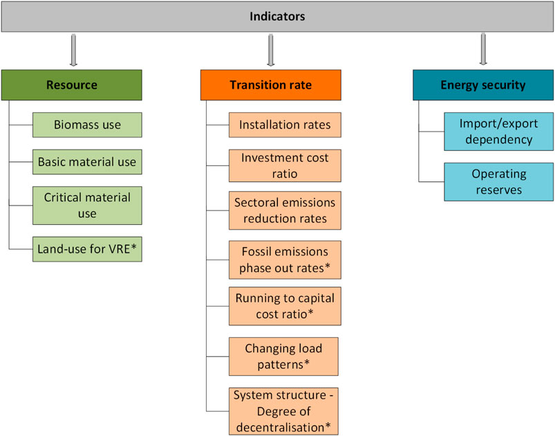
FIGURE 1. Schematic overview of the indicators. Indicators marked with an asterisk are presented in the Supplementary Material.

Resource Indicators

Biomass Use

The magnitude of the sustainable biomass supply for future energy purposes depends on such factors as the willingness to pay for biomass in different sectors, population growth, diets, technological developments, crops used, requirements and views related to biodiversity (Slade et al., 2014). Thus, it is unclear as to how much biomass will be available for the electricity sector and at what cost. To estimate the dependency on biomass in the various scenarios, we calculate the yearly biomass used in the modelling scenarios (EJ) per region r and compare this to the estimates of sustainable biomass potentials in the region (ESBP) in EJ/yr (de Wit and Faaij, 2010). Since the latter is a subject for debate, it becomes even more important to contextualise the biomass demand in modelling. The biomass use rate (BUR) is calculated as:

$BU{R}_{r,y}=\frac{B{U}_{r,y}}{ESBP}(1)$

where BU is the biomass usage in region r, in year y, and ESBP is the estimated sustainable biomass potential. Although outside the scope of the present work, it will be important to derive this indicator for all sectors that aspire to using biomass, i.e., the industry, transport and heating sectors. In a climate-constrained world, there will most likely be different levels of willingness to pay for biomass. It should also be mentioned that when it comes to forestry-derived biomass this is typically used in a cascading way, reflecting the willingness of Society to pay for different biomass products. Thus, biomass for energy purposes currently exists in the form of residues from the forest industry. In a world that is developing in line with the Paris Agreement, the cascading order may change depending on how Society values different activities, and whether and to what extent these can substitute for the use of carbon-based fuels and feedstocks (Berndes et al., 2018).

Basic Material Use

The growth of renewable energy technologies needed for an energy transition inevitably entails increased demand for certain resources (IEA, 2020). While previous studies have focused primarily on the roles of critical minerals in a low-carbon transition (Vidal et al., 2013; Moss et al., 2018; Boubault and Maïzi, 2019), here we focus on the implications for basic materials. Renewable energy technologies, such as wind and solar energy, are more metal-intensive than current energy sources, with wind turbines requiring high-grade primary steel (Davidsson et al., 2014). Moreover, the construction of wind turbines involves a substantial need for concrete foundations. Furthermore, an energy system with a high level of non-dispatchable Variable Renewable Energy (VRE) could increase the need for transmission capacity, which is also material-intensive (Jorge et al., 2012a; Jorge et al., 2012b). To assess the natural resources demand, we calculate the additional demands for metals and concrete based on the power capacity added and the transmission capacities installed on an annual basis, taking into account the replacement needed for power capacities. We use the average material use per MW of wind power (divided into on-shore and off-shore) and the two main options for transmission capacity: overhead lines or cables buried in trenches (including substations and transformers) (Harrison et al., 2010; Jorge and Hertwich, 2013). The material demand (MD) is, thus, calculated as:

$M{D}_{u,r,y_n}={\displaystyle \sum }_{t}M{U}_{u,t}\ast \left(NI{C}_{t,r,y_n}+NI{C}_{t,r,y_{n-30}}\right)+{\displaystyle \sum }_{tt}M{U}_{u,tt}\ast NI{C}_{tt,r,y_n}(2)$

where $M{D}_{u,r,y_n}$ is the demand for material u, consisting of cement, steel, aluminium and copper, in region r in year y_n; $MU$ is the use of material u per MW of wind power for generation technology t, consisting of on-shore and off-shore wind, and for transmission technology tt, consisting of overhead lines or cables in trenches; and NIC is the new installed capacity of generation technology t or transmissions technology tt in region r in years n. The material use indicator presented here has an important application in determining what the different energy technologies in scenarios obtained from energy systems modelling (in the present paper, electricity generation) will require in terms of material use [e.g., metals as investigated by Kleijn et al. (2011)], in comparison to today’s material production levels.

Critical Material Uses and Scale-Up of Batteries

Batteries in the electricity system can be used in two forms: stationary and electric vehicle (EV) batteries. Stationary batteries can be used to reduce the total system cost by storing electricity from hours of low net-load [i.e., electricity generation from VRE minus demand] to hours with high net-load. EV batteries can be used to power the EV when driving, as well as to store the electricity through vehicle-to-grid systems or to absorb electricity at low or negative net-load hours when the vehicles are parked. The current ability to manufacture batteries, as well as to provide enough critical materials (mainly cobalt, vanadium and lithium in today’s battery chemistries), is limited (Alves Dias et al., 2018).

The first indicator, called the battery production ratio (BPR), highlights the challenge of producing the amount of economically profitable battery capacity required by the models. It is calculated as:

$BP{R}_{r,y}=\frac{BC{I}_{r,y}}{BP{C}_{r,y=2019}}(3)$

where BCI is the amount of battery capacity installed in the model per region and year and BPC is the battery production capacity per region in the current year (2019). Newly installed batteries per year include both new batteries and the replacement of old EVs and stationary batteries.

The second indicator, termed the critical material ratio (CMR), highlights the challenge of providing the quantity of critical materials needed for battery production. It is calculated as:

$CM{R}_{r,y,cm}=\frac{CM{U}_{r,y,cm}}{CMR{e}_{r,cm}}(4)$

where CMU is the cumulative amount of critical material cm needed in a region r up to a certain year y for producing EV and stationary batteries, and CMRe represents the reserves of critical material in the modelled region (critical material reserve). We used cobalt and vanadium as two examples of critical materials used currently in battery production. The indicator CMR can be used in the same way for other types of (critical) materials, for example the lithium used in batteries, neodymium and dysprosium used in wind power production, and indium and selenium used for solar PV production. Furthermore, there is a potential for recycling critical materials, thereby, extending their lifespans and reducing the CMU. A recycling rate of 90% for cobalt and vanadium is assumed in the calculation of the CMU (Alves Dias et al., 2018). Even though the recycling potential of batteries is >90% for many of the materials, given the use of new recycling technologies and the presence of a suitable infrastructure for battery collection and full-scale recycling plants (Andersson et al., 1016), there is a high risk that the recycled materials from batteries will be used as carrier metals, construction materials, and back-filling materials or will be land-filled in many countries instead of their metal properties being utilised (e.g., in new batteries) (Author anonymous, 2019a).

Transition Rate Indicators

Installation Rates

Decarbonisation of the electricity system will require a rapid ramping up of low-CO₂ electricity generation capacity. The rate of deployment of low-carbon technologies may give an indication of the plausibility of a given scenario, where rapid uptake of a certain technology over a short period of time in a country or region may call for closer scrutiny. Napp et al. (2017) have identified a number of factors to consider when assessing technology penetration rates, including the availability of supporting technologies, lead time to build technology and the availability of financial and human capital, skills and supply chains. While historical development is not necessarily a good guide of future development, a common approach to assessing the viability of the rate of change suggested in a scenario is to use historical growth rates as benchmarks. Several different measures of the rate of deployment of new electricity generation capacity are used in the literature (Sovacool, 2008; Wilson et al., 2013; van Sluisveld et al., 2015; Cao et al., 2016; Napp et al., 2017), including measures of absolute growth (ΔGW/yr, ΔTWh/yr) and relative or normalised growth [average annual growth (% change), GW/yr/GDP, kWh/cap/yr]. Here, for each scenario, we calculate the annual installation rates (ΔGW/yr) and average annual growth rates (%) for each technology in each country and region. For the key technologies, we also provide an estimate of the number of installations required. The average annual added capacity (ΔC) for each technology is calculated as:

$\Delta C_{t,r}=\frac{I{C}_{t,r,y_n}-I{C}_{t,r,y_m}}{y_n-y_m}(5)$

where IC is the installed capacity of technology t in region r in year (y) m and n. The average annual growth rate (G) is calculated as:

$G_{t,r}={\left(\frac{I{C}_{t,r,y_n}}{I{C}_{t,r,y_m}}\right)}^{\frac{1}{y_n-y_m}}-1(6)$

where, again, IC is the installed capacity of technology t in region r in year (y) m and n.

Investment Cost Ratio

For a large-scale transition, significant levels of new investments are needed. We choose the investment cost to GDP (ICtGDP) ratio for the analysis and define it as the ratio between the investment cost in the electricity generation capacities and GDP:

$\text{ICtGDP}=\frac{{{\displaystyle \sum }}_{\text{t}}\text{I}\_{\text{Cost}}_{\text{t},\text{ c},\text{y}}}{{\text{GDP}}_{\text{c},\text{y}}}(7)$

where, $I\_Cos{t}_{t,c,y}$ is the investment cost of a generation technology $t$ in country $c$ and year $y$, and $GD{P}_{c,y}$ is the GDP of country $c$ in year $y$. The GDP projections up to Year 2050 are extracted from the Shared Socioeconomic Pathways 2 (Riahi et al., 2017). It should be noted that in the present work investment costs (in ICtGDP) differ from the capital costs, such that the investment costs in a given year comprise the real (not annualised) investments in the technologies invested in that year, while the capital costs in a given year include annualised investments in all the technologies with life-times spanning that year. Financial investments in the energy system will depend on many parameters related to public and private spending and the conditions of the financial markets. Furthermore, investments in the energy sector are likely to boost economic activity, create new jobs reduce different environmental costs, making investment cost and GDP interdependent and not independent factors. Thus, the indicator in Eq. 7 should only be regarded as a first measure to compare the required future investments with historical spending.

Sectoral Emissions Reduction Rates

It is expected that the electricity sector will support other sectors, such as the industry, transport, and heat sectors, in their decarbonisation efforts via electrification. Thus, the sectoral CO₂ emissions intensity indicator is important to assess the progress of decarbonisation and to track the transition towards fully decarbonised sectors.

The CO₂ intensity of the given electricity system is defined as the ratio of CO₂ emissions from the fuel inputs of the electricity generation technologies to the total electricity demand. Thus, the Electricity Emission Intensity (EEI) is calculated as:

$EE{I}_{r,h,y}=\frac{{{\displaystyle \sum }}_t\left(\frac{E{G}_{t,r,h,y}}{{\eta }_t}E{F}_t\right)}{D_{r,h,y}}(8)$

where EG is the electricity generation of technology t, in region r, at hour h and year y, η is the efficiency of technology t, EF is the emissions factor of the fuel, and D is the electricity demand in region r, at hour h and year y.

The sectoral CO₂ emissions intensity (SEI) is calculated as the total CO₂ emissions that arise from sector activity relative to sectoral demand:

$SE{I}_{r,y}^s=\frac{{{\displaystyle \sum }}_h\left(EE{I}_{r,h,y}\ast SE{D}_{r,h,y}\right)+SE{I}_{r,y}^{noEl}{s}_{r,y}\left(1-i_{r,y}\right)}{S{D}_{r,y}^s}(9)$

where SEI is the total sectoral CO₂ intensity in region r and year y, and SED is the sectoral electricity demand in region r, at hour h and year y. $SE{I}^{noEl}$ is the CO₂ intensity of the non-electrified part of the sector, $S{D}^s$ is the total sectoral demand, and i represents the share of the electrified sector in region r and year y.

For the sake of simplicity, it is assumed that the emissions from the non-electrified shares of the sectors will remain at current levels for all years. In reality, these emissions are also likely to be reduced. Sectoral electrification rates were taken from a previous publication (Göransson et al., 2021). More details on the calculation of sectoral CO₂ intensities can be found in Supplementary Appendix A3.

Energy Security Indicators

Import/Export Dependency

Energy security, which is an integral part of energy policy, encompasses many different aspects, with one important dimension being availability (Cherp and Jewell, 2011). Azzuni and Breyer (2018) have defined availability using three parameters: the regional availability of energy resources; energy infrastructure; and energy consumers. The latter refers to accessibility to consumers who can utilise energy generated within the region. In this paper, we quantify two parameters that are related to this definition of availability, namely the import and export dependencies in regions with regards to electricity. The import dependency is defined as the share of the total demand in the region that is met by imported electricity, and the export dependency is the share of total generated electricity within a region that is required to be exported to other regions. The import and export dependencies can, thus, be said to concern all three of the availability parameters stated above, with energy resources and energy infrastructure being related to import dependency. Thus, a low import dependency indicates the availability of good VRE conditions and a high level of infrastructure in the region that can supply the regions demand. A high export dependency indicates a low availability of consumers in the region in relation to power generation, and that the region is dependent upon access to consumers in other regions. When calculating the dependencies, it is important to adopt a time resolution that can capture variations, both in the generation from non-dispatchable technologies and in demand. A too-coarse time resolution risks hiding intra-period needs for import and export. The equations for import dependency (ID) and export dependency (ED) over a year with hourly resolution are:

$I{D}_r=\frac{{{\displaystyle \sum }}_{h}N{I}_{h,r}}{{{\displaystyle \sum }}_h{D}_{h.r}}(10)$

$E{D}_r=\frac{{{\displaystyle \sum }}_{h}N{E}_{h,r}}{{{\displaystyle \sum }}_{h}E{G}_{h.r}}(11)$

where NI_h,i (net import) and NE_h,i (net export) are the positive net total amounts of electricity imported and exported in each time-step and in each region, respectively. Thus, for a specific time-step, a region has a positive NI with NE being zero, a positive NE with NI being zero, or both values are zero. D denotes the electricity demand and EG represents the electricity generation. There are, of course, also other parameters that are relevant for energy security, such as diversification of fuel imports. Therefore, the indicators presented here should be complemented with additional indicators related to energy security, such as changes caused to imports/exports by other energy carriers, e.g., nuclear fuel and biomass.

Operating Reserves

To ensure reliable on-demand electricity, the system requires some reserve capacity to compensate for unforeseen events, forecast errors, as well as normal variations in supply and demand. While these reserves can be designed for several time-scales (primary, secondary and tertiary reserves), only secondary reserves are analysed here, as an example. We perform a post-modelling analysis by looking at the frequency, duration, and distribution of events with critically low operational reserves. The level of operating reserves required in high-VRE systems is difficult to estimate without statistical analysis of the historical operation (a challenging task for modelled future scenarios), and it depends on the exact composition of the system. Nevertheless, the reserves required to manage typical load variations can be estimated using either historical data or heuristic formulas. Here, we use the latter type, calculating the reserves (R) as:

$R_d=\sqrt{a\ast L_{d, max}+b^2}-b(12)$

where $L_{d, max}$ is the maximum hourly demand during day $d$, and a and b are parameters used to tune the correlation between daily load and reserve requirements. This equation was used to take into account the fact that different regions have vastly different load-levels in accordance with the ENTSO-E Operation Handbook (ENTSOE, 2015), so as to calculate the secondary control reserve with a = 10 MW and b = 150 MW. These values are used also in the present study and result in approximately 200–500 MW of required reserves in the studied regions. For reference, Sweden has a total reserve demand of 573 MW according to the Swedish TSO.

To estimate available secondary reserves, we assume that online units can ramp up to some extent (20–50%), whereas hydropower and online gas turbines ramp up fully. Furthermore, stationary batteries can contribute as reserves with the energy that is not used for energy arbitrage throughout the day. Lastly, any curtailment also counts as available reserves.

Model Description

The indicators in this work are designed to quantify the implications of the results obtained from electricity system investment models. In this study, we use a semi-heuristic, cost-minimising electricity system investment model, called Hours-to-Decades (H2D), to illustrate the results from the indicators (Göransson, 2019). In the H2D model, the investment decision is solved for 2-weeks segments, thereby spanning the duration of wind variations that frequently occur in the range of 8 days at the hub height of modern turbines (Sørensen, 2017). There is a 3-hour time resolution within each 2-weeks segment. The 2-weeks segments are run in parallel and the generation, storage and transmission capacity investments of each segment are collated to form the basis for the investment cost distribution between the 2-weeks segments in subsequent model runs. Through iterative solving, the 2-weeks segments converge in terms of generation, storage, and transmission capacity expansion. The model includes a representation of the existing electricity and heat generation infrastructure, as well as its age profile. A full description of the model is available elsewhere (Göransson, 2019). The segmentation of the year into 2-weeks pieces allow the H2D model to combine a high temporal resolution with a high level of technical detail and a large geographical scope. However, it also restrains the model from assessing the size of seasonal storages. And while an evaluation of the modelling methodology shows that the final electricity system suggested by the H2D model has a total system cost close to the cost-optimal system composition, the embedded heuristics in the methodology does not guarantee optimality (Göransson et al., 2021).

The H2D model includes several aspects of what we here refer to as variation management (Göransson and Johnsson, 2018), including thermal cycling, H₂ storage, heat storage and stationary battery storage. Storage is dispatched such that the storage level in the last time-step in the 2-week period equals the storage level in the first time-step of the same 2-week period. The full range of generation and storage technologies considered in this study, and the properties thereof, can be found in Supplementary Appendix A2. In addition, variation management through electrification of electrification of the iron ore reduction process in the steel-making industry the steel-making industry and passenger vehicles, as well as the replacement of fossil fuels for residential heating is included and further described elsewhere (Göransson et al., 2021). Electrification of other industrial sectors is not considered in this study.

Scenarios

The geographical scope considered in this work is Northern Europe, and includes Denmark, Estonia, Finland, Germany, Ireland, Latvia, Lithuania, the Netherlands, Norway, Poland, Sweden, and the United Kingdom. The countries are subdivided into 12 regions to represent major transmission bottlenecks, as shown in Supplementary Appendix Figure A1.1. Trade across the geographical scope is allowed, and investments in new transmission capacities among regions is possible. The temporal scope of the study is three decades (2030, 2040 and 2050), where each decade is represented by 1 year in the model. The existing power-plant fleet, as given by the continuously updated Chalmers Power Plant Database (Kjärstad and Johnsson, 2007), is taken as a starting point, and generation capacity is gradually phased out as the present power plants reach their technical end-of-life, although the use of power plants may be discontinued before this if they become un-economical. The main difference between the studied decades is the increase that occurs in the cost of CO₂, starting at 40 EUR/tonne in 2030, increasing to 100 EUR/tonne in 2040, and reaching 400 EUR/tonne in 2050. The 2030 level correspond to projects made on ETS market prices (Schjølset, 2014). However, recent estimates point to that the 2040 level, as applied here, could be attained already in 2030 (Shankleman, 2021). The 2050 level is set to effectively disincentivise electricity generation associated with CO₂ emissions. The cost of CO₂ affects both the operation of existing plants and new investments in the electricity system (as well as the operation thereof). However, electricity generation capacity already in place remains available until the technical life-time is reached. Electricity demand from electrification of the steel industry and passenger vehicles, together with the replacement of fossil fuels with electricity for heating (using heat pumps with a coefficient of performance of 3) is added to the current electricity demand in respective region, as explained in a previous paper (Göransson et al., 2021). Overall, this electrification results in an additional electricity demand of around 900 TWh per year by 2050 for the regions investigated, corresponding to an increase in electricity demand of around 50%.

Two main scenarios are considered in this work: the Collaboration and No Collaboration scenarios. Whereas scenarios in previous work mainly differ in degree of electrification (European Commission, 2018; IEA, 2018), these scenarios differ in terms of how demands for electricity and heat from the transport, industry and heat sectors are being integrated into the electricity and district heating systems. This differentiation between the two scenarios is made possible by the high temporal resolution and degree of technical detail of the H2D model. Table 1 summarises the differences between the scenarios. In the No Collaboration scenario, the new demands for heat and electricity have a predefined temporal distribution (i.e., no load shifting is assumed). EVs recharge their batteries directly whenever they are parked for 6 h or longer. The charging is only limited by the charging capacity, i.e., 3.7 kWh per hour, and does not consider the availability or price of electricity. The electricity required to produce H₂for the steel-making process is in the No Collaboration scenario evenly distributed across the hours of the year. Furthermore, in the No Collaboration scenario, natural gas for heating is replaced by individual heat pumps located in the individual buildings and operated according to the heat demand profile of the households.

TABLE 1

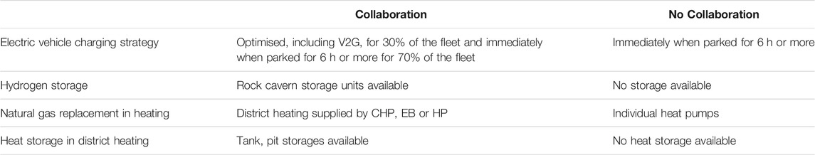
TABLE 1. Differences between the Collaboration and No Collaboration scenarios.

In contrast, in the Collaboration scenario, EV charging is always flexible in relation to time for 30% of the vehicles, while still meeting the driving demand for transportation. It is also possible for these EVs to discharge back to the grid (i.e., vehicle-to-grid; V2G). The remaining 70% of the EVs still charge as soon as they are parked for 6 hours or more. As for the steel industry, in the Collaboration scenario, there is an option to make additional investments in electrolyser capacity and H₂ storage. Natural gas for heating is in this scenario replaced by district heating. The heat demand for district heating can be met by combined heat and power (CHP) plants, electric boilers (EB), and heat pumps (HP). There is also the possibility to invest in thermal tank and pit storages (TES Tank and TES Pit). No current national or regional policies are included in this study such as achieving carbon neutrality before 2050. Further details on scenarios can be found elsewhere (Göransson et al., 2021).

Results and Discussion

Basic Scenario Results

We show that collaboration between the electricity system and an electrified steel industry, passenger vehicles and household heat supply can reduce total system costs by 8% compared to the No Collaboration scenario, under the assumptions made in this work. However, the Northern European electricity system composition is found to be dominated by wind power, irrespective of whether sectorial collaboration is available. Figure 2A shows the annual levels of electricity generation in Northern Europe under the two scenarios in the years investigated, and the corresponding capacities are given in Figure 2B. In Year 2050, inter-sectoral collaboration increases the share of the demand supplied: from 61 to 63% for wind power; and from 16 to 19% for solar PV. The largest difference between the scenarios investigated is the way in which the variability is managed. Figure 2C gives the energy storage capacities for the scenarios considered. In the No Collaboration scenario, the high share of VRE sources is achieved through large investments in stationary battery capacity (Figure 2C), together with the operation of combined-cycle and open-cycle gas turbines (Figure 2B). Consequently, around 700 GWh of stationary batteries are expected to be in place by Year 2050. In the Collaboration scenario, stationary batteries play a negligible role in managing variations of generation. Instead, these variations are managed by flexible H₂ production and strategic EV charging, enabled by investments in H₂ storage and strategic operation of the vehicle batteries, respectively. The batteries of the EVs provide flexibility without compromising their primary purpose of providing transportation, and it is here assumed that the flexibility provision to the grid does not degrade the battery substantially (i.e., no costs are associated with this flexibility provision). In the Collaboration scenario, demand-side flexibility not only reduces the need for stationary batteries, but also reduces the need for flexible generation. Flexible generation, in the form of combined-cycle gas turbines, support the electricity system during periods of prolonged low-level wind power generation, from Year 2030 and onwards. Natural gas-fired combined-cycle gas turbines dominate flexible generation up to Year 2040. However, in Year 2050 they are replaced with biogas-fired combined-cycle gas turbines in both scenarios. By Year 2050, biogas-based electricity generation is 32 TWh higher per year in the No Collaboration scenario than in the Collaboration scenario. The total biogas-based electricity production corresponds to 6–7% of the annual electricity demand. While the cost of biomass can be expected to increase with the demand for biomass in the transport and industry sector, previous work has shown that a small share of bio-based electricity generation has a very high value as a complement to wind and solar power (Johansson et al., 2019). For more detailed results for the scenarios regarding system composition and operation, the reader is directed to the previous paper (Göransson et al., 2021).

FIGURE 2

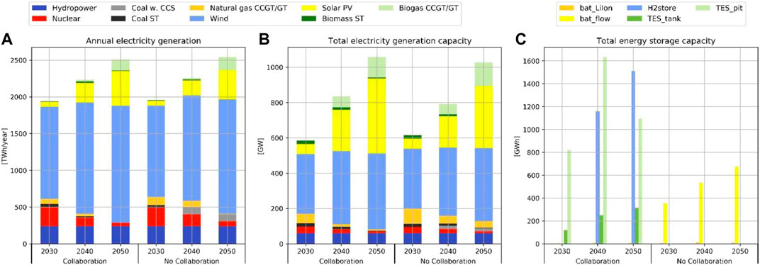
FIGURE 2. Modelling results, as obtained from the two scenarios investigated in this work. (A) The annual electricity generation; (B) the total installed electricity generation capacity; and (C) the total energy storage capacity, for the two scenarios for Years 2030, 2040 and 2050. CCS, Carbon capture and storage, here with biomass blending for zero total emissions; CCGT, combined-cycle gas turbine; ST, steam turbine; H2store, hydrogen storage; TES, thermal energy storage; bat_Lion, Li-ion stationary batteries; bat_flow, flow stationary batteries. The batteries in electric cars are not included in this graph.

Resource Indicators

Biomass Use

Biomass use in the electricity system is low in Year 2030 and Year 2040 (less than 0.3 EJ) but increases significantly by Year 2050, reaching 0.86 EJ in the Collaboration scenario and 0.93 EJ in the No Collaboration scenario, corresponding to ca. 17.3 and 18.6%, respectively, of the estimated sustainable biomass supply in the whole studied region (de Wit and Faaij, 2010) (Figure 3). Most of the biomass is used in only two regions, where it compensates for limitations associated with other resources, i.e., in the southern United Kingdom region, which has a high electricity demand and relatively low VRE resource potential, and in the southern Germany region, which also has limited wind potential. For comparison, according to EUROSTAT, 0.78 EJ of biomass were used in the entire studied region in Year 2018 for electricity and combined heat and power production, with the main users of biomass being Germany (0.33 EJ), the United Kingdom (0.13 EJ), and Sweden (0.09 EJ). An assessment of used biomass sustainability is not available. This level of biomass usage is significantly higher than that obtained from the modelling for Years 2030 and 2040 (cf.Figure 3), which indicates that conversion to a VRE-based electricity system may temporarily reduce the need for biomass in the electricity system. Nonetheless, biomass will play an important role in balancing the electricity system when near-zero emissions are reached and a large share of the future sustainable biomass could be needed for that purpose. Yet, due to the limited scope of the model used here, the value of biomass for the electricity system should be compared to the value of biomass for other sectors, to ensure a thorough appraisal. In addition, it is not obvious to what extent biomass can be reallocated between regions in terms of import/export. Ideally, the biomass should be sourced to the regions that display the highest level of willingness to pay for the biomass (i.e., having the greatest need for this fuel). Overall, it should be noted that the modelling results are cost-optimal solutions, so they will not reflect the real development, where considerations other than cost are included. Although it seems unlikely that biomass-fired units will to a large extent be phased out until Year 2030, the modelling shows that other types of generation are more cost-efficient.

FIGURE 3

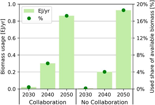
FIGURE 3. The amounts of biomass (left axis) used in the modelled region in the two scenarios in Years 2030, 2040 and 2050, and including (right axis) this usage as a percentage of the estimated sustainable biomass in the region.

Basic Material Use

Steel and concrete/cement are the main basic materials used in the construction of most systems for electricity generation capacity (except solar PV). In the present study, we focus on the material use associated with wind power, as this generation technology dominates the expanded generation capacity of the coming decades in the model. Additional transmission capacity also implies the increased use of basic materials, predominantly in the forms of aluminium and copper, both of which are used in transmission cables, substations and transformers. As shown in Figure 4, the levels of material use for wind power and transmission technologies are highest over the present decade (2020–2030). The expected annual level of material use for the energy transition is equivalent to around 10% of the annual consumption of copper in the EU, while corresponding to around 2% of EU steel and aluminium consumption and less than 1% of the annual consumption of cement in the EU. While the overall levels of material use for the entire region do not demonstrate large differences between the two scenarios, there are substantial differences between the scenarios for individual regions. In Sweden, for example, the amount of steel required for the expansion of wind capacity up to Years 2040 and 2050 for the No Collaboration scenario is almost double than that for the Collaboration scenario. In both cases, a high demand for steel can be expected beyond Year 2050 when the wind turbines built in Year 2030 will need to be replaced. Obviously, there is a need to relate the transition of the energy system to the needs for materials and other resources. This will have important implications for different industries and their associated value chains in terms of what they can expect in the future, given different scenarios. This will likely entail both opportunities for material suppliers (as in the current example) and challenges such as increased competition (resulting in increased prices) for raw materials (such as iron ore for steel production).

FIGURE 4

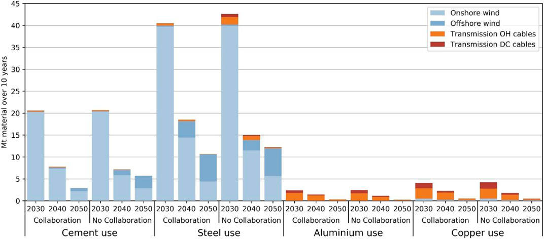
FIGURE 4. Material usage of base materials in the analysed scenarios.

Critical Material Uses and Scale-Up of Batteries

The lithium-ion EV battery manufacturing capacity globally was 200 GWh/yr in 2019 (Author anonymous, 2019b). The average cobalt content of a battery is about 0.36 kg/kWh based on the current battery chemistries. The average amount of vanadium in flow batteries (an option to invest in stationary applications in the model) is about 5.2 kg/kWh (Zhang et al., 2016). The cobalt and vanadium global reserves amount to 18 and 22 Mtonnes, respectively, of which around 10% (1.8 Mtonnes) and <1% (<0.2 Mtonnes), respectively, are located in the modelled region (Alves Dias et al., 2018). Table 2 shows the number of stationary and EV batteries produced and the results for the two indicators: the BPR (i.e., the required battery capacity divided by the current production capacity) and the CMR, in the two scenarios for the entire modelled region in Years 2030, 2040 and 2050.

TABLE 2

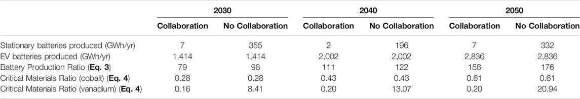
TABLE 2. The numbers of stationary and electric vehicle (EV) batteries produced, the battery production ratios, and the Critical Materials ratios for the Collaboration and No Collaboration scenarios in Years 2030, 2040 and 2050.

The BPR differs to some extent between the No Collaboration and Collaboration scenarios, although in both scenarios it indicates the need for about 80-times the current production capacity in the modelled region already by Year 2030 (Table 2) and the need for up to 20% more battery capacity in the No Collaboration scenario, as compared to the Collaboration scenario. The investments in stationary batteries in the No Collaboration scenario are small compared to the investments needed in EV battery capacity for the transport sector. In the No Collaboration scenario, around 883 GWh of stationary batteries are invested in the modelled region by Year 2050, as compared to 6 TWh of EV batteries (assuming electrification rates for passenger cars of 50% by Year 2030, 70% by Year 2040, and 100% by Year 2050, and a battery capacity size of 30 kWh). These batteries, obviously, have as their main purpose to power transportation. However, since the driving profiles exploit the EV batteries for only a fraction of their maximum potential, the EV batteries can also serve the stationary electricity system. Yet, it is most important to limit the EV battery capacity size, even though using the capacity of EV batteries instead of that of stationary batteries will further reduce the total level of battery capacity (transport and stationery) needed.

As shown in Table 2, by 2050, in both scenarios, the amount of cobalt needed for the construction of EV batteries is 61%% of the cobalt reserves within the modelled region. The region will need about 6% of all the cobalt reserves currently available globally, and the current fleet in the region corresponds to about 10% of the current global passenger fleet. However, the present study assumes a high recycling rate of 90%. In addition, the cobalt in EV batteries corresponds to about 50% of the current global market for cobalt. Furthermore, it seems likely that passenger cars will not be the only user of batteries in the transport sector. In 2016, 126,000 tonnes of cobalt were mined in 20 countries around the world. The main countries with mining of cobalt are the Democratic Republic of Congo, Russia and Australia. In Europe, cobalt production in Year 2016 was estimated at 2,300 tonnes, all of which was sourced from Finland (Alves Dias et al., 2018).

As shown in Table 2, vanadium reserves are scarcer than cobalt reserves in the region. As a consequence, vanadium needs to be imported to cover the heavy demand for stationary batteries in the No Collaboration scenario. In this study, the amount of cobalt and vanadium in current battery chemistries is used, as well as, the current estimates of the reserves. New battery chemistries that reduce the use of cobalt and vanadium or diminish recycling of the critical materials (if no additional reserves that can be sustainably extracted are found) are therefore needed.

Transition Indicators

Installation Rates

As illustrated in Figure 5A, both scenarios show a rapid uptake of wind and solar power. In the first decade (2020–2030) on-shore wind power predominates, with an average annual installation rate of almost 25 GW/yr. After Year 2030, solar PV installation rates increase significantly to more than 20 GW/yr in the Collaboration scenario and to 16–19 GW/yr in the No Collaboration scenario. This is partly a model artefact. A known weakness of optimisation models is the “Penny-switching” effect, in which small changes in input parameters may lead to considerable changes in the output (DeCarolis et al., 2017). Here, this means that the model chooses to invest initially in favourable wind locations and subsequently in more costly PV capacity (2030–2040). These results can be compared with the historical installation rates. In the period 2010–2018, the average annual installation rates of wind power in the studied region as a whole (which accounted for 60% of the total installed capacity of wind power in the EU-27 in Year 2018) ranged from 5 GW/yr (in Year 2010) to approximately 12 GW/yr (in Year 2016) (IRENA, 2019). In the same period, the average annual additions of solar PV ranged from 3 GW/yr (in Year 2016) to 9 GW/yr (in Year 2011) (IRENA, 2019). Thus, the progress of the energy transition is accelerating in the scenarios investigated here. Yet, these values are not excessively high compared to the historical values and, thus, the suggested installation rates should be feasible in most regions.

FIGURE 5

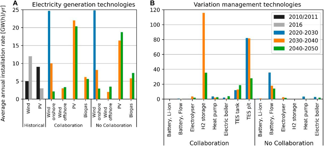
FIGURE 5. Average annual installation rates for: (A) electricity generation capacity (GW/yr); and (B) variation management technology capacity (GW(h)/yr). The graphs shows the average annual capacity additions in the period 2020–2050 for the entire region modelled in the Collaboration scenario and No Collaboration scenario, respectively.

The thermal power plant’s share of total electricity generation decreases in both scenarios (cf.Figure 2). However, more than 5 GW/yr of biogas combined-cycle capacity is brought online in both scenarios during the period 2030–2050. In addition, in the No Collaboration scenario, in the period of 2030–2040, 1.8 GW/yr of co-fired thermal power plants equipped with CCS (Bio-coal CCS) are installed.

As the share of VRE sources increases, the importance of energy storage and of other technologies to support variation management increases. Figure 5B shows how the installation rates of variation management technologies, including storage, differ between the two scenarios. In the Collaboration scenario, which allows investments in both hydrogen storage (H₂ storage) and thermal energy storage (TES Tank and TES Pit), the average annual installation rate of H₂ storage is approximately 116 GWh/yr in the period 2030–2040 and 35 GWh/yr in 2040–2050. The thermal energy storage capacity also increases significantly, with more than 80 GWh of pit heat storage capacity being added annually in the periods 2020–2030 and 2030–2040. In the No Collaboration scenario, where H₂ storage and thermal energy storage is not available, flow batteries become important to handle storage and variation management. In the period 2020–2030, approximately 35 GWh of flow battery capacity are installed each year. Thereafter, the installation rates decline. As the capacities for all of the energy storage and variation management technologies discussed here will increase from initially low levels, comparisons with historical installation rates are less relevant. Instead, specification of the performance of existing systems will here be used to provide a point of reference. For long-term and large-scale storage of H₂, underground storage in salt caverns or lined rock caverns seems most favourable. Based on information about the salt cavern H₂ storage facilities in operation today (six worldwide) and in the commissioning phase (IEA, 2018; Caglayan et al., 2020), an estimated storage capacity of 50–150 GWh seems reasonable. This would mean that 1 or 2 such H₂ storage facilities would need to be deployed each year in the Collaboration scenario during the period 2030–2040. It is worth noting that more than 100 caverns are in use today for the storage of natural gas for seasonal load balancing and as reserves (Caglayan et al., 2020). The storage method and costs may vary significantly between regions due to differences in geological conditions (Andersson and Grönkvist, 2019). The total capacity of existing installations for seasonal storage of heat is approximately 0.5 GWh for TES Tanks and in the range of 5–15 GWh for TES Pits (Gibb et al., 2018). This means that in the Collaboration scenario, 5–16 pit storages would need to be commissioned each year.

The average annual growth rates (%) could be used as a complementary performance indicator, and this would give an indication of the outliers in the scenarios. As shown in Supplementary Appendix A4.4, the average annual growth rates can be used to spot the rapid relative growth of a certain technology in a certain region, as well as extensive change in a certain country (cf. Cherp et al., 2021).

Investment Cost Ratio

The modelling results show that investments in electric power generation technologies in the region modelled in the scenarios investigated constitute a small fraction of the region’s GDP. The total region’s ICtGDP (investment cost-to-GDP) ratio initially increases and then decreases from around 0.8% in Year 2030 down to around 0.18% in Year 2050 in both scenarios. This can be compared to 0.2–0.3% of the GDP spent on power plants around Year 2010 (average between Year 2005 and Year 2014) (IEA, 2016). The most significant change is observed for the Baltic countries, in which the ICtGDP ratio is around 3% (in both scenarios) in Year 2030 due to a dramatic increase in wind power capacity, up from the historical level of around 0.4% in Year 2010. Thereafter, it declines to 0.0 and 0.2% in Year 2050 in the Collaboration and No Collaboration scenarios, respectively, as all valuable wind areas will be exploited by Year 2030. These values, together with the results for the electricity import/export dependency of the investigated countries (cf.Section 4.4.1), indicate that from the Northern European perspective it is economically justifiable for the Baltic states, as well as for foreign investors, to divert significant resources into the electric power sector already by Year 2030, so as to export electricity to the neighbouring regions in the future. The results also show that changes in the ICtGDP ratios between other regions and investigated years are less drastic (see Supplementary Appendix Table A4.7.1, Supplementary Appendix A for the ICtGDP ratios for the investigated countries).

Sectoral Emission Reduction Rates

Figure 6A shows carbon intensity of the electricity sector, electric passenger vehicles, electrified residential heating and steelmaking with hydrogen reduction. As mentioned in DescriptionofIndicators, for simplicity, it is assumed that emissions from the non-electrified shares of each sector will remain on the current levels throughout the period investigated. The CO₂ emissions intensity of the electricity system is 11 and 28% lower in the Collaboration scenario than in the No Collaboration scenario in years 2030 and 2040, respectively. The electricity system of 2050 in the Collaboration scenario is fully decarbonized, but in the No Collaboration scenario, CO₂ emissions still arise from electricity generation. The CO₂ intensities are 55 and 34% lower for electrified passenger vehicles and the steel-making industry, respectively, and 3% higher for electrified heating in the Collaboration scenario than in the No Collaboration scenario. In 2030 and 2040, the electrified residential heat is the most carbon-intense sector of the electrified sectors in both scenarios, since heat consumption occurs when the remaining fossil fuel-based electricity generation technologies are running. Figures 6B–D, show the total CO₂ intensities of the residential heating, passenger vehicles, and steel-making industry, expressed as kgCO₂/km for vehicles (Figure 6B), kgCO₂/KWh for heating (Figure 6C), and kgCO₂/tonne for steel (Figure 6D), respectively. By Year 2050, the steel industry and passenger vehicles are fully decarbonized. In Year 2050, the CO₂ intensity of residential heating is 18 gCO₂/kWh_heat in both scenarios, given that 9% of residential heating is still supplied by fossil fuels. Disaggregation of the sectoral CO₂ emissions trends reveals striking differences between sectors and regions (Price et al., 1998), and provides insights for the further development of decarbonisation. The indicator can be further improved by considering electricity trading across regions and the charging and discharging of storage units.

FIGURE 6

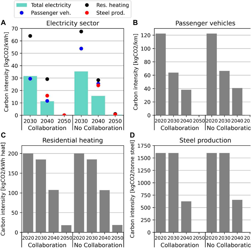
FIGURE 6. Total carbon dioxide emissions intensities of: (A) the electricity system and electrified sectors (industry, transport, and heat sector); (B) the transport sector, in gCO₂/km; (C) the heat sector, in gCO₂/kWh_heat; (D) the industry sector, in kgCO₂/tonne steel, for different scenarios and years.

Energy Security Indicators

Import/Export Dependency

Figure 7 shows the annual import and export dependencies of a select number of regions for the modelled years and the historical period 2016–2019 for the Collaboration and No Collaboration scenarios, respectively (for the results for all regions see Supplementary Appendix Tables A4.11.1, A4.11.2). For the modelled years, both the import and export dependencies vary considerably between regions, with southern Sweden (SE_S) reaching up to 70% and down to 0% in import dependency and export dependency, respectively, and the Baltic (BAL) region reaching 2 and 70%, respectively. Overall, there are more regions with high export dependency than regions with high import dependency, indicating that the energy consumer aspect of energy availability, i.e., the access to consumers for the energy producers, may be of greater concern than the resource and infrastructure aspects for most regions in the investigated scenarios. The differences between the scenarios are minor, with the largest difference seen for the import dependency of Norway (NO), which is 15–20 percentage points higher in the No Collaboration scenario because Norwegian hydropower is used more extensively for balancing. For the other regions, the differences between the scenarios for both the export and import dependencies are in the range of 0–8 percentage points. The small difference between scenarios indicates that policy choices that promote one scenario or the other do not affect the import or export dependencies.

FIGURE 7

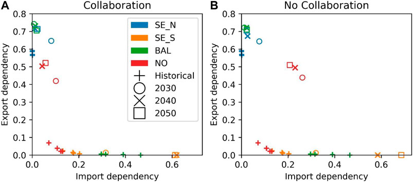
FIGURE 7. The annual export and import dependencies for the modelled period and the period of 2016–2019 (“historical”) in selected regions (different colours) in: (A) the Collaboration scenario; and (B) the No Collaboration scenario. The results for all the regions are presented in Supplementary Appendix Tables A4.11.1, A4.11.2.

Some regions show considerable deviations from the historical values. The BAL region currently has a relatively high import dependency (30–46%) and essentially no export dependency. In the modelled scenarios, this situation changes considerably, with import dependency dropping to around 1–2% and export dependency increasing to just over 70%. Similar changes can be seen in Norway (NO), with export dependency increasing from the current rate of around 10% to around 50% in Year 2050, and southern Sweden (SE_S) where the import dependency increases from the current level of 20% to 60–70% in Year 2050. The substantial changes in both the import and export dependencies are due to shifts in system composition from, primarily, thermal power plants, which are placed near the demand, to VRE sources for which the location is more-dependent on the resource potential in different regions. This indicates that the possible future scenarios modelled in this work will have weaker energy security than the current system, with regards to electricity as an energy carrier.

Operating Reserves

The system requires some reserve capacity that can compensate for unforeseen events and forecast errors, as well as compensate for variations in supply and demand. The heuristic formula given by Eq. 11 is used to estimate the required reserves at approximately 200–500 MW for the studied systems. Figure 8 illustrates the violations of minimum operational reserve capacity for the northern United Kingdom region for different years and scenarios. The figure shows the available reserves throughout the year in the form of a bar-code plot, in which the red lines indicate hours of no available reserves and the orange lines indicate some, albeit insufficient, levels of reserves. A large difference can be seen between the two scenarios, in that the No Collaboration scenario rarely has any available reserves while the Collaboration scenario almost always has sufficient reserves. For the northern United Kingdom region, this difference is due to the storage units used. The No Collaboration scenario has flow battery storage, which is cycled almost once per day, while the Collaboration scenario uses EV batteries with far fewer full cycles (in terms of aggregated battery storage). Since only excess energy at the end of the day is considered eligible for reserves during the same day, the aforementioned difference in storage technology generates the difference in available reserves shown in Figure 8. It should be noted that this specific region is a significant net-exporter of power, which over-estimates the effects associated with assuming that reserves must be supplied locally within the producing region. Regardless of whether or not the evaluation of available reserves should be adjusted to account for trade, Figure 8 clearly highlights the fact that the two scenarios have significantly different prerequisites for providing reserves. The results for all the regions and scenarios are given in the Supplementary Appendix Figures A4.12.1, A4.12.2.

FIGURE 8

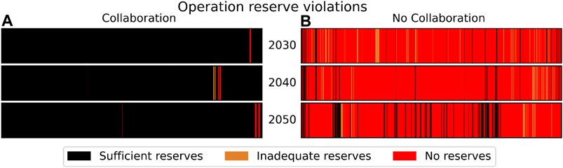
FIGURE 8. The violations of minimum operational reserve capacity for the northern United Kingdom region for different years and scenarios. The red and orange lines indicate the hours of no or low reserves, respectively. Panel (A) shows the operational reserve violations for the Collaboration scenario, while panel (B) shows the violations for the No Collaboration scenario.

Conclusions and Policy Implications

In this paper, we propose and exemplify indicators that can facilitate the interpretation of the scenario results from energy systems modelling and thereby enhance the basis for policy-making. We focus on the electricity system transition, for which we provide modelling results for two different scenarios for northern Europe, together with 13 indicators, divided into resource, transition rate, and energy security indicators. Together, these indicators highlight areas in which indirect costs and other considerations can play significant roles in shaping the future energy system.

We show that while the large-scale expansion of wind and solar power in the scenarios investigated seems feasible from the material and land-use perspectives, upscaling of VRE in some regions implies the need to raise capital for energy investments that are substantially larger than those presently put into the energy infrastructure. Furthermore, the benefit of utilising sector coupling for flexibility provision, rather than dedicated stationary batteries, is found to be motivated not only by costs but also by the availability of scarce minerals and the provision of reserve generation. The indicators also show that the modelling methodology has a limited ability to provide results that render advice as to installation rates, ignoring the problems linked to intense periods of material usage interrupted by decades of much lower material usage. This is similar to the real world, in which cycles of boom and bust are common in industry. Yet, the results presented here should not be seen as a predictor of market behaviour.

We argue that using various indicators that address different aspects of the expected large-scale expansion of the electricity system based on VRE sources and sectoral integration facilitates: 1) communication of the results and their consequences–both opportunities and challenges–to policy-makers; 2) understanding the consequences of the energy system transformation in a wider context; 3) avoiding suboptimal solutions that could result from ignoring specific aspects or focusing exclusively on one aspect; and 4) assisting internal reviews and discussions around modelling results within and between modelling groups. It is likely that trade-offs as well as synergies exist within each scenario, and these should be understood to make informed political decisions.

The indicators presented in this work should be regarded as examples. They may need to be refined, as well as complemented with other indicators, depending on which policies are in focus (see for example Liu, 2014; Kouloumpis et al., 2015; Rösch et al., 2017; Azzuni and Breyer, 2018). Nonetheless, providing more detailed results for model scenarios via indicators should make the results more accessible for discussions in wider audiences, as well as to scientists in other fields (e.g., social sciences), thereby allowing further analyses of the political and social feasibilities of the results. This is particularly important because there are many aspects of the energy transition that are not explicitly considered in the models and, thus, are also not part of the optimisation. The indicators can also serve as a basis for analysing the energy transition in a wider sustainability perspective, for example to support the quantification of the UN Sustainable Development Goals (SDGs). Given that the indicators aim to help non-energy modellers in their understanding of the results from energy system models, they should be tested and discussed with these actors. Such cross-disciplinary exercises can help modellers to formulate better indicators and help non-modellers to understand more clearly the types of information that can be derived from energy system models. In summary, we believe that indicators of the type exemplified in this work represent a way to make energy system models more suitably adapted to providing well-grounded decision support.

The choice and presentation of the indicators in this work were to some extent guided by the model structure and resolution that was used to produce the analysed scenarios. Other indicators may be more relevant when using more detailed country-level models. It is also important to bear in mind the system boundaries when interpreting results. For example, with more stringent climate targets, there will be many sectors that will want to use biomass to reduce their emissions. This will result in higher biomass prices and in uncertainty regarding the amount of biomass available for the electricity system. Therefore, the present scenario analysis only considers part of the energy system and, thus, can provide insights into the cost-effective use of biomass within those boundaries. The same applies to other limited resources that are used in several sectors.

It should also be kept in mind that most future scenarios cover increasing levels of electrification in different sectors, reflecting the fact that the whole system is expanding and covering more energy services over time. This means that more investments will be needed, as compared to the historical rates, although comparisons to these can help to grasp the magnitude of effort required to materialise such electricity systems.

Furthermore, the indicators presented here were not part of the optimisation but were applied ex post, i.e., the indicators did not influence the optimisation. Integrating indicators into the modelling optimisation process and investigating synergies and dependencies among them are possible further developments of such analysis. However, as mentioned in the introduction to this paper, to make the indicators part of the optimization would be a highly complex task due the different areas they cover and their interdependencies. Yet, the authors of this work believes that the ex post use of indicators can be an efficient tool for highlighting challenges important for policy-makers or scientist from other fields such as when the indicator values in future scenarios diverge considerably from historical values. This implies that it would be valuable to add model constrains to investigate the consequences of limiting the indicator. Thus, the indicators also serve an important function in evaluating scenario designs and modelling tools in general. More dynamic inclusion of constraints was developed for example by Sole et al. (2020). Yet, these applications tend to have other limitations such as limited representation of technology dispatch.

In summary, we argue that these types of indicators should be further developed and widely used to make modelling results more accessible and useful for managing the transition on the policy level, as well as for internal evaluations of the scenarios produced, especially if the target audience is broader than the scientific community. Quantification of indicators enables discussions within modelling groups regarding the appropriateness of the tools to answer posed questions, as well as in policy-making to understand the trade-offs and synergies between different solutions and to foster a deeper understanding of the issues in the electricity system. In both cases, these types of indicators can help to illuminate the limitations of the scenarios developed and the limitations of the modelling methods used. This paper should be seen as a starting point for developing indicators and as a call to other modellers to develop further the list of indicators and apply a selection of them based on research question at hand to their scenarios.

Data Availability Statement

The raw data supporting the conclusions of this article will be made available by the authors, without undue reservation.

Author Contributions

FJ conceived the idea, LG provided the model data for analysis, VH, IK, ML, EN, MO, DR, JR, MT, AT, JU, KV, and VW developed indicators and analysed the results, ML supervised the process. All authors contributed to the writing of the paper.

Funding

This project was partially funded by North European Energy Perspectives Project (NEPP) www.nepp.se.

Conflict of Interest

The authors declare that the research was conducted in the absence of any commercial or financial relationships that could be construed as a potential conflict of interest.

Publisher’s Note

All claims expressed in this article are solely those of the authors and do not necessarily represent those of their affiliated organizations, or those of the publisher, the editors and the reviewers. Any product that may be evaluated in this article, or claim that may be made by its manufacturer, is not guaranteed or endorsed by the publisher.

Supplementary Material

The Supplementary Material for this article can be found online at: https://www.frontiersin.org/articles/10.3389/fenrg.2021.677208/full#supplementary-material

References

Author anonymous, (2019b). Recycle Spent Batteries. Nat. Energy 4, 253. doi:10.1038/s41560-019-0376-4

CrossRef Full Text | Google Scholar

Author anonymous, (2019a). Recycle Spent Batteries. Nat. Energ. 4(4), 253–253.

CrossRef Full Text | Google Scholar

Alves Dias, P., Blagoeva, D., Pavel, C., and Arvanitidis, N. (2018). Cobalt: Demand-Supply Balances in the Transition to Electric Mobility. Luxembourg: JRC.

Anderson, K., and Jewell, J. (2019). Debating the Bedrock of Climate-Change Mitigation Scenarios. Nature 573, 348–349. doi:10.1038/d41586-019-02744-9

PubMed Abstract | CrossRef Full Text | Google Scholar

Andersson, J., and Grönkvist, S. (2019). Large-scale Storage of Hydrogen. Int. J. Hydrogen Energ. 44 (23), 11901–11919. doi:10.1016/j.ijhydene.2019.03.063

CrossRef Full Text | Google Scholar

Andersson, M., Ljunggren Söderman, M., and Sandén, B. A.Are Scarce Metals in Cars Functionally Recycled? Waste Manag. 60, 407–416. doi:10.1016/j.wasman.2016.06.031

PubMed Abstract | CrossRef Full Text | Google Scholar

Azzuni, A., and Breyer, C. (2018). Definitions and Dimensions of Energy Security: a Literature Review. Wires Energ. Environ. 7 (1), e268. doi:10.1002/wene.268

CrossRef Full Text | Google Scholar

Badea, A. C., Rocco S., C. M., Tarantola, S., and Bolado, R. (2011). Composite Indicators for Security of Energy Supply Using Ordered Weighted Averaging. Reliability Eng. Syst. Saf. 96 (6), 651–662. doi:10.1016/j.ress.2010.12.025

CrossRef Full Text | Google Scholar

Behrens, P., van Vliet, M. T. H., Nanninga, T., Walsh, B., and Rodrigues, J. F. D. (2017). Climate Change and the Vulnerability of Electricity Generation to Water Stress in the European Union. Nat. Energ. 2 (8), 17114. doi:10.1038/nenergy.2017.114

CrossRef Full Text | Google Scholar

Berndes, G., Goldmann, M., Johnsson, F., Lindroth, A., Wijkman, A., Abt, B., et al. (2018). Manage for Maximum wood Production or Leave the forest as a Carbon Sink? Kungl. Skogs- Och Lantbruksakademiens Tidskrift. 6, 157.

Google Scholar

Berrill, P., Arvesen, A., Scholz, Y., Gils, H. C., and Hertwich, E. G. (2016). Environmental Impacts of High Penetration Renewable Energy Scenarios for Europe. Environ. Res. Lett. 11 (1), 014012. doi:10.1088/1748-9326/11/1/014012

CrossRef Full Text | Google Scholar

Boubault, A., and Maïzi, N. (2019). Devising Mineral Resource Supply Pathways to a Low-Carbon Electricity Generation by 2100. Resources 8 (33). doi:10.3390/resources8010033

CrossRef Full Text | Google Scholar

Caglayan, D. G., Weber, N., Heinrichs, H. U., Linßen, J., Robinius, M., Kukla, P. A., et al. (2020). Technical Potential of Salt Caverns for Hydrogen Storage in Europe. Int. J. Hydrogen Energ. 45 (11), 6793–6805. doi:10.1016/j.ijhydene.2019.12.161

CrossRef Full Text | Google Scholar

Cao, J., Cohen, A., Hansen, J., Lester, R., Peterson, P., and Xu, H. (2016). China-U.S. Cooperation to advance Nuclear Power. Science 353 (6299), 547–548. doi:10.1126/science.aaf7131

PubMed Abstract | CrossRef Full Text | Google Scholar

Cherp, A., Vinichenko, V., Tosun, J., Gordon, J. A., and Jewell, J. (2021). National Growth Dynamics of Wind and Solar Power Compared to the Growth Required for Global Climate Targets. Nat. Energy 6 (7), 742–754. doi:10.1038/s41560-021-00863-0

CrossRef Full Text | Google Scholar

Cherp, A., and Jewell, J. (2011). The Three Perspectives on Energy Security: Intellectual History, Disciplinary Roots and the Potential for Integration. Curr. Opin. Environ. Sustain. 3 (4), 202–212. doi:10.1016/j.cosust.2011.07.001

CrossRef Full Text | Google Scholar

Davidsson, S., Grandell, L., Wachtmeister, H., and Höök, M. (2014). Growth Curves and Sustained Commissioning Modelling of Renewable Energy: Investigating Resource Constraints for Wind Energy. Energy Policy. 73, 767–776. doi:10.1016/j.enpol.2014.05.003

CrossRef Full Text | Google Scholar

de Wit, M., and Faaij, A. (2010). European Biomass Resource Potential and Costs. Biomass. Bioenergy 34 (2), 188–202. doi:10.1016/j.biombioe.2009.07.011

CrossRef Full Text | Google Scholar

DeCarolis, J., Daly, H., Dodds, P., Keppo, I., Li, F., McDowall, W., et al. (2017). Formalizing Best Practice for Energy System Optimization Modelling. Appl. Energ. 194, 184–198. doi:10.1016/j.apenergy.2017.03.001

CrossRef Full Text | Google Scholar

Eichhorn, M., Masurowski, F., Becker, R., and Thrän, D. (2019). Wind Energy Expansion Scenarios - A Spatial Sustainability Assessment. Energy 180, 367–375. doi:10.1016/j.energy.2019.05.054

CrossRef Full Text | Google Scholar

ENTSOE (2015). Operation Handbook.

European Commission (2018). A Clean Planet for All: A European Strategic Long-Term Vision for a Prosperous, Modern, Competitive and Climate Neutral Economy, Brussels: European Commission.

European Commission (2019). Communication from the Commission to the European Parliament, the European Council, the Council, the European Economic and Social Committee of the Regions, The European Green Deal COM/2019/640 final, Brussels: European Commission.

Fürsch, M., Hagspiel, S., Jägemann, C., Nagl, S., Lindenberger, D., and Tröster, E. (2013). The Role of Grid Extensions in a Cost-Efficient Transformation of the European Electricity System until 2050. Appl. Energ. 104, 642–652. doi:10.1016/j.apenergy.2012.11.050

CrossRef Full Text | Google Scholar

García-Gusano, D., Iribarren, D., Martín-Gamboa, M., Dufour, J., Espegren, K., and Lind, A. (2016). Integration of Life-Cycle Indicators into Energy Optimisation Models: the Case Study of Power Generation in Norway. J. Clean. Prod. 112, 2693–2696. doi:10.1016/j.jclepro.2015.10.075

CrossRef Full Text | Google Scholar

Gibb, D., Johnson, M., Romani, J., Gasia, J., Gabeza, L. F., and Gurtner, R. (2018). Applications of Thermal Energy Storage in the Energy Transition – Benchmarks and Developments. International Energy Agency’s Technology Collaboration Programme.

Göransson, L. (2019). A Parallel Computing Approach to Account for Wind Power Variation Management in Electricity System Investment Models. submitted for publication.

Göransson, L., Granfeldt, C., and Strömberg, A.-B. (2021). Management of Wind Power Variations in Electricity System Investment Models. SN Operations Res. Forum. 2 (2), 1–30. doi:10.1007/s43069-021-00065-0

CrossRef Full Text | Google Scholar

Göransson, L., and Johnsson, F. (2018). A Comparison of Variation Management Strategies for Wind Power Integration in Different Electricity System Contexts. Wind Energy 21 (10), 837–854. doi:10.1002/we.2198

CrossRef Full Text | Google Scholar

Hammond, G. P., Howard, H. R., and Jones, C. I. (2013). The Energy and Environmental Implications of UK More Electric Transition Pathways: A Whole Systems Perspective. Energy Policy 52, 103–116. doi:10.1016/j.enpol.2012.08.071

CrossRef Full Text | Google Scholar

Harrison, G. P., Maclean, E. J., Karamanlis, S., and Ochoa, L. F. (2010). Life Cycle Assessment of the Transmission Network in Great Britain. Energy Policy 38 (7), 3622–3631. doi:10.1016/j.enpol.2010.02.039

CrossRef Full Text | Google Scholar

IEA (2020). Clean Energy Progress after the Covid-19 Crisis Will Need Reliable Supplies of Critical Minerals. Paris.

IEA (2016). World Energy Outlook.

IEA (2018). World Energy Outlook 2018. IEA.

IRENA (2019). Renewable Capacity Statistics 2019. Abu Dhabi.

Iribarren, D., Martín-Gamboa, M., Navas-Anguita, Z., García-Gusano, D., and Dufour, J. (2020). Influence of Climate Change Externalities on the Sustainability-Oriented Prioritisation of Prospective Energy Scenarios. Energy 196, 117179. doi:10.1016/j.energy.2020.117179

CrossRef Full Text | Google Scholar

Johansson, V., Lehtveer, M., and Göransson, L. (2019). Biomass in the Electricity System: A Complement to Variable Renewables or a Source of Negative Emissions? Energy 168, 532–541. doi:10.1016/j.energy.2018.11.112

CrossRef Full Text | Google Scholar

Jorge, R. S., Hawkins, T. R., and Hertwich, E. G. (2012). Life Cycle Assessment of Electricity Transmission and Distribution-Part 1: Power Lines and Cables. Int. J. Life Cycle Assess. 17 (1), 9–15. doi:10.1007/s11367-011-0335-1

CrossRef Full Text | Google Scholar

Jorge, R. S., Hawkins, T. R., and Hertwich, E. G. (2012). Life Cycle Assessment of Electricity Transmission and Distribution-Part 2: Transformers and Substation Equipment. Int. J. Life Cycle Assess. 17 (2), 184–191. doi:10.1007/s11367-011-0336-0

CrossRef Full Text | Google Scholar

Jorge, R. S., and Hertwich, E. G. (2013). Environmental Evaluation of Power Transmission in Norway. Appl. Energ. 101, 513–520. doi:10.1016/j.apenergy.2012.06.004

CrossRef Full Text | Google Scholar

Kjärstad, J., and Johnsson, F. (2007). The European Power Plant Infrastructure-Presentation of the Chalmers Energy Infrastructure Database with Applications. Energy Policy 35 (7), 3643–3664. doi:10.1016/j.enpol.2006.12.032

CrossRef Full Text | Google Scholar

Kleijn, R., van der Voet, E., Kramer, G. J., van Oers, L., and van der Giesen, C. (2011). Metal Requirements of Low-Carbon Power Generation. Energy 36 (9), 5640–5648. doi:10.1016/j.energy.2011.07.003

CrossRef Full Text | Google Scholar

Kouloumpis, V., Stamford, L., and Azapagic, A. (2015). Decarbonising Electricity Supply: Is Climate Change Mitigation Going to Be Carried Out at the Expense of Other Environmental Impacts? Sustainable Prod. Consumption 1, 1–21. doi:10.1016/j.spc.2015.04.001

CrossRef Full Text | Google Scholar

Kruyt, B., van Vuuren, D. P., de Vries, H. J. M., and Groenenberg, H. (2009). Indicators for Energy Security. Energy Policy 37 (6), 2166–2181. doi:10.1016/j.enpol.2009.02.006

CrossRef Full Text | Google Scholar

Lehtveer, M., and Hedenus, F. (2015). Nuclear Power as a Climate Mitigation Strategy - Technology and Proliferation Risk. J. Risk Res. 18 (3), 273–290. doi:10.1080/13669877.2014.889194

CrossRef Full Text | Google Scholar

Lehtveer, M., Makowski, M., Hedenus, F., McCollum, D., and Strubegger, M. (2015). Multi-criteria Analysis of Nuclear Power in the Global Energy System: Assessing Trade-Offs between Simultaneously Attainable Economic, Environmental and Social Goals. Energ. Strategy Rev. 8, 45–55. doi:10.1016/j.esr.2015.09.004

CrossRef Full Text | Google Scholar

Liu, G. (2014). Development of a General Sustainability Indicator for Renewable Energy Systems: A Review. Renew. Sust. Energ. Rev. 31, 611–621. doi:10.1016/j.rser.2013.12.038

CrossRef Full Text | Google Scholar

Louis, J.-N., Allard, S., Debusschere, V., Mima, S., Tran-Quoc, T., and Hadjsaid, N. (2018). Environmental Impact Indicators for the Electricity Mix and Network Development Planning towards 2050 - A POLES and EUTGRID Model. Energy 163, 618–628. doi:10.1016/j.energy.2018.08.093

CrossRef Full Text | Google Scholar

Moss, R. L., Tzimas, E., Kara, H., Willis, P., and Kooroshy, J. (2018). Critical Metals in Strategic Energy Technologies - Assessing Rare Metals as Supply-Chain Bottlenecks in Low-Carbon Energy Technologies. Netherlands: European Commission Joint Research Centre – Institute for Energy and Transport: Pettens.

Napp, T., Bernie, D., Thomas, R., Adam Hawkes, J., and Gambhir, A. (2017). Exploring the Feasibility of Low-Carbon Scenarios Using Historical Energy Transitions Analysis. Energies 10 (1), 116. doi:10.3390/en10010116

CrossRef Full Text | Google Scholar

Neumann, F., and Brown, T. (2021). The Near-Optimal Feasible Space of a Renewable Power System Model. Electric Power Syst. Res. 190, 106690. doi:10.1016/j.epsr.2020.106690

CrossRef Full Text | Google Scholar

Peng, W., Wagner, F., Ramana, M. V., Zhai, H., Small, M. J., Dalin, C., et al. (2018). Managing China's Coal Power Plants to Address Multiple Environmental Objectives. Nat. Sustain. 1 (11), 693–701. doi:10.1038/s41893-018-0174-1

CrossRef Full Text | Google Scholar

Pfenninger, S., Hawkes, A., and Keirstead, J. (2014). Energy Systems Modeling for Twenty-First century Energy Challenges. Renew. Sust. Energ. Rev. 33, 74–86. doi:10.1016/j.rser.2014.02.003

CrossRef Full Text | Google Scholar

Pratama, Y. W., Purwanto, W. W., Tezuka, T., McLellan, B. C., Hartono, D., Hidayatno, A., et al. (2017). Multi-objective Optimization of a Multiregional Electricity System in an Archipelagic State: The Role of Renewable Energy in Energy System Sustainability. Renew. Sust. Energ. Rev. 77, 423–439. doi:10.1016/j.rser.2017.04.021

CrossRef Full Text | Google Scholar

Price, L., Worrell, E., Khrushch, M., and Michaelis, L., (1998). Sectoral Trends and Driving Forces of Global Energy Use and Greenhouse Gas Emissions. Mitigation Adaptation Strateg. Glob. Change 3 (2), 263–319. doi:10.1023/a:1009695406510

CrossRef Full Text | Google Scholar

Pye, S., Broad, O., Bataille, C., Brockway, P., Daly, H. E., Freeman, R., et al. (2021). Modelling Net-Zero Emissions Energy Systems Requires a Change in Approach. Clim. Pol. 21 (2), 222–231. doi:10.1080/14693062.2020.1824891

CrossRef Full Text | Google Scholar

Riahi, K., van Vuuren, D. P., Kriegler, E., Edmonds, J., O’Neill, B. C., Fujimori, S., et al. (2017). The Shared Socioeconomic Pathways and Their Energy, Land Use, and Greenhouse Gas Emissions Implications: An Overview. Glob. Environ. Change 42, 153–168. doi:10.1016/j.gloenvcha.2016.05.009

CrossRef Full Text | Google Scholar

Rösch, C., Bräutigam, K.-R., Kopfmüller, J., Stelzer, V., and Lichtner, P. (2017). Indicator System for the Sustainability Assessment of the German Energy System and its Transition. Energ Sustain. Soc. 7 (1), 1. doi:10.1186/s13705-016-0103-y

CrossRef Full Text | Google Scholar

Schjølset, S. (2014). The MSR: Impact on Market Balance and Prices. Thomson Reuters.

Schlachtberger, D. P., Brown, T., Schäfer, M., Schramm, S., and Greiner, M. (2018). Cost Optimal Scenarios of a Future Highly Renewable European Electricity System: Exploring the Influence of Weather Data, Cost Parameters and Policy Constraints. Energy 163, 100–114. doi:10.1016/j.energy.2018.08.070

CrossRef Full Text | Google Scholar

Shankleman, J. (2021). Major New Climate Report Puts Pressure on COP26 to ‘Consign Coal to History’. Bloomberg.

Slade, R., Bauen, A., and Gross, R. (2014). Global Bioenergy Resources. Nat. Clim Change 4, 99–105. doi:10.1038/nclimate2097

CrossRef Full Text | Google Scholar

Solé, J., Samsó, R., García-Ladona, E., García-Olivares, A., Ballabrera-Poy, J., Madurell, T., et al. (2020). Modelling the Renewable Transition: Scenarios and Pathways for a Decarbonized Future Using Pymedeas, a New Open-Source Energy Systems Model. Renew. Sust. Energ. Rev. 132, 110105. doi:10.1016/j.rser.2020.110105

CrossRef Full Text | Google Scholar

Sørensen, B. (2017). Renewable Energy -Physics, Engineering, Environmental Impacts, Economics and Planning. Academic Press.

Sovacool, B. K. (2008). Valuing the Greenhouse Gas Emissions from Nuclear Power: A Critical Survey. Energy Policy 36 (8), 2940–2953. doi:10.1016/j.enpol.2008.04.017

CrossRef Full Text | Google Scholar

Sovacool, B. K. (2016). How Long Will it Take? Conceptualizing the Temporal Dynamics of Energy Transitions. Energ. Res. Soc. Sci. 13, 202–215. doi:10.1016/j.erss.2015.12.020

CrossRef Full Text | Google Scholar

van Sluisveld, M. A. E., Harmsen, J. H. M., Bauer, N., McCollum, D. L., Riahi, K., Tavoni, M., et al. (2015). Comparing Future Patterns of Energy System Change in 2 °C Scenarios with Historically Observed Rates of Change. Glob. Environ. Change 35, 436–449. doi:10.1016/j.gloenvcha.2015.09.019

CrossRef Full Text | Google Scholar

Vandepaer, L., Panos, E., Bauer, C., and Amor, B. (2020). Energy System Pathways with Low Environmental Impacts and Limited Costs: Minimizing Climate Change Impacts Produces Environmental Cobenefits and Challenges in Toxicity and Metal Depletion Categories. Environ. Sci. Technol. 54 (8), 5081–5092. doi:10.1021/acs.est.9b06484

PubMed Abstract | CrossRef Full Text | Google Scholar

Vidal, O., Goffé, B., and Arndt, N. (2013). Metals for a Low-Carbon Society. Nat. Geosci. 6 (11), 894–896. doi:10.1038/ngeo1993

CrossRef Full Text | Google Scholar

Wilson, C., Grubler, A., Bauer, N., Krey, V., and Riahi, K. (2013). Future Capacity Growth of Energy Technologies: Are Scenarios Consistent with Historical Evidence? Climatic Change 118 (2), 381–395. doi:10.1007/s10584-012-0618-y

CrossRef Full Text | Google Scholar

Zhang, X., Li, Y., Skyllas-Kazacos, M., and Bao, J. (2016). Optimal Sizing of Vanadium Redox Flow Battery Systems for Residential Applications Based on Battery Electrochemical Characteristics. Energies 9 (10), 857. doi:10.3390/en9100857

CrossRef Full Text | Google Scholar

Glossary

BUR Biomass use rate

BU Biomass usage

ESBP Estimated sustainable biomass potential

MD Material demand

MU Material use

NIC New installed capacity

BPR Battery production ratio

BCI Battery capacity installed

BPC Battery production capacity

CMR Critical material ratio

CMU Cumulative material use

CMRe Critical material reserve

ΔC Average annual added capacity

IC Installed capacity

G Average annual growth rate

ICtGDP Investment costs to GDP

I_Cost Investment costs

GDP Gross Domestic Product

EEI Electricity emission intensity

EG Electricity generation

η Efficiency of generation technologies

EF Emission factor

D Electricity demand

SEI Sectoral emissions intensity

SED Sectoral electricity demand

i Share of the electrified sector

SD Final sectoral demand

ID Import dependency

NI Net import

ED Export dependency

NE Net export

R Reserves

L Maximum hourly demand

LU Land use

CD Capacity density

LA Land area

p Phase out rate

E Produced energy

RtCC Running-to-Capital Costs ratio

RC Running costs

CC Capital costs

corr Correlation factor

Xg Ratio of decentralised/centralised generation over the total generation

Xd Ratio of decentralised/centralised electricity demand over the total electricity demand

Xs Ratio of decentralised/centralised energy storage volume over the total energy storage volume

S Total energy storage volume

Xt Ratio between centralised cross-regional trade and the total electricity generation.

T Cross-regional trade

r region

y year

u basic materials

t technology

tt transmission technology

cm critical material

c country

h hour

d day

n,m indexes for different time periods

a parameter used to tune the correlation between daily load and reserve requirements

b parameter used to tune the correlation between daily load and reserve requirements