A residential user classification approach based on the graded portrait with considering the IDR adaptability and potential

1 Introduction

In the recent years, due to the diversified developments of the electricity demand of residential users, the amount of the residential power consumption has risen sharply (Siavash et al., 2018; Li et al., 2019; Yoshida et al., 2020). The randomness and uncertainty of the power consumption behaviors of the residential users significantly cause the peak and valley loads in the power system, which may severely impact the security, stability, and economy of the system. However, it can be obviously seen that along with the increasing amount of the residential power consumption, the proportion of the flexible residential load is also increasing, which has become a kind of remarkable regulating resource on the user side (Alrumayh and Bhattacharya, 2019; Chen et al., 2021). Therefore, to relieve the pressure of the balance between the power supply and the user demand, as well as to guarantee the security, stability, and economy of the power system, the residential user level demand response (DR) has received more and more attentions. Among various related studies (Asadinejad et al., 2017; Sandels et al., 2019; Lee et al., 2020), the DR based portrait and classification for analyzing the user power consumption behaviors have been reported as the effective ways for serving the auxiliary load regulations (Zhu et al., 2020; Guan et al., 2021). The basic idea of the researches is to identify if the residential user is suitable for participating in DR according to the power consumption behavior (represented by the load curve) revealed by the portrait and classification algorithms. And then, the suitable users will be selected to finally join the DR tasks. However, it should be pointed out that the current existing portrait algorithms and the classification algorithms lack of considerations for different DR characteristics among various residential users, which cannot be conveniently employed in the complicated residential user-level DR scenarios. As a result, for developing the portrait algorithm and the classification algorithm specially serving DR applications, DR scenarios should be regarded as the crucial elements. Therefore, the residential users with different DR characteristics for serving different DR scenarios are able to be identified, according to the customized differentiated DR strategies for different users.

DR is frequently categorized into two types including the price demand response (PDR) and the incentive demand response (IDR) (Song et al., 2020; Assad et al., 2022). Compared to PDR, IDR has increasingly become an effective way for serving the load shifting in the power system due to its outstanding quick-response ability and capacity-expansion ability, which has been widely used in the intraday and real-time dispatches (Laitsos et al., 2021; Vahedipour-Dahraie et al., 2022). The economic incentive is able to induce the customer to sign the IDR contract with the electric power company. Based on the contract, the user can actively adjust the power consumption pattern to reduce the electricity consumption when load peaks emerge in the power system, whilst gaining a proper cost compensation (Wu et al., 2022). However, because of the unique features of the IDR contraction for example the strong timeliness, it puts forward higher requirements for the characteristics of the power consumption behaviors of the candidate participating users. According to the previous researches (Gaba and Chanana, 2021; Wang et al., 2022), the IDR adaptability of the residential user including historical load level, power consumption regularity, power consumption volatility, and responding willingness can be employed to assess the response reliability. In order to identify the users with better IDR adaptabilities, research (Ahir and Chakraborty, 2022) presented an evaluation method based on the characteristics of the user’s power consumption pattern and the historical load level. The presented methods are able to fully consider and model the consumers’ power consumption habits in IDR. However, it cannot clearly distinguish the users’ groups with respect to the IDR response capacity. Research (Liang and Ma, 2021) firstly focused on analyzing the differences of IDR response capacities under different load modes. And then, the research further employed the indices including the power consumption regularity and the historical load level to evaluate the actual response abilities of the users participating in IDR under different load modes. The authors claimed that the IDR participators can select the appropriate load modes from the presented methods according to various practical demands. However, the willingness of the user is also an important characteristic which impacts the implementation of identifying the user’s IDR adaptability. Although the aforementioned researches have shown the effectiveness of identifying the user’s IDR adaptability for participating in the IDR, the IDR invitation initiated by the power company is usually located in a specific one to 2 h in a day. In this case, the identified suitable users using the above methods may have quite little response capacities in the short periods of time. Or it can be summarized that the IDR potentials of the users are relatively low. Therefore, to assess the IDR potential of a user, and further to assist the power company in properly dispatching the demand side resources, the portrait approach of the user IDR potential with considering more comprehensive features should be developed. Research (Qi et al., 2020) evaluated the user IDR potential based on the adjustable capacity, which is computed using the load difference before and after the IDR participation of the user. The authors reported that based on their research, the user IDR potential can be quantified during the IDR period. Research (Weitzel and Glock, 2019) firstly computed the desired level of load reduction based on the load reduction curves of the beforehand generated IDR invitation period. And then, the adjustable capacity is further employed to assess the user IDR potential. The authors also claimed that the adjustable capacity is able to help to estimate the potential of the user.

The portrait is able to delineate if a user is suitable to participate in IDR. However, in the practical dispatch, among an enormous number of users, the power company should also be aware of what kind of user is suitable to participate in IDR efficiently. Therefore, based on the portrait of the user IDR potential, and further combining the portrait of the IDR adaptability, the labeling of the residential users can be carried out. As a result, by employing the deep learning algorithms, the residential users with high IDR adaptabilities and high IDR potentials could be efficiently and effectively identified. Consequently, the power company can explicitly dispatch these kinds of residential users to serve IDR. At present, the supervised machine learning algorithms and the deep learning algorithms are widely used in the user load classification researches (Zhou et al., 2013; Jiang et al., 2018; Chen et al., 2021). However, it has been pointed out that although the lower complexities of the traditional supervised machine learning algorithms result in higher classification efficiency, because of lacking of sufficient layer-wise complexity and the nonlinear mapping process (Agiollo and Omicini, 2021), they cannot supply satisfied feature transformation and learning abilities which the deep learning algorithms for example deep belief network (DBN) can provide contrarily. Researches (Liu et al., 2020; Phyo and Jeenanunta, 2021; Arvanitidis et al., 2022) adopted back propagation neural network (BPNN), multilayer perceptron (MLP), and DBN to classify the load dataset. The authors indicated that in terms of classification accuracy, DBN significantly outperforms the traditional machine learning based supervised classification algorithms. The authors further admitted that the time sequence load data with high dimensions frequently encounters the training difficulty using DBN. This point finally impacts the efficiency of the classification. To solve the issues caused by the high-dimensional load data, several researches (Jing and Ying, 2019; Li and Chen, 2020; Yin et al., 2021) aimed at developing the classifiers especially for serving the time sequence data. However, other researchers (Paul and Chalup, 2017; Chen et al., 2020) suggested that the dimension reduction is also an effective way to solve the issue of processing high-dimensional load data. Currently, the usually used dimension reduction algorithms include the characteristic index dimension reduction (CIDR), singular value decomposition (SVD), and principal component analysis (PCA) (Wan and Yu, 2020; Huang et al., 2021; Chen et al., 2022). Although these algorithms are able to provide high efficiency in terms of dimension reduction, the information loss of the original data is quite severe (Anowar et al., 2021; Ray et al., 2021). As a result, the load classification accuracy could be significantly impacted. Research (Kingma and Welling, 2014; Gunduz, 2021) innovatively employed variational autoencoder (VAE) to deal with the dimension reduction task. VAE is able to learn the distribution characteristics of the high-dimensional data based on its unique coding and decoding mechanisms. Therefore, the dimension reduction can be conveniently implemented, whilst retaining the original data characteristics as far as possible. The authors claimed that the effectiveness of VAE can be observed based on their experimental results. Researches (Lin et al., 2020; Wei et al., 2021) also proved the adaptability of VAE for handling the dimension reduction operations.

Motivated by the previous researches and the anxiety of the efficient identification of the users with high IDR adaptabilities and potentials, this paper presents a residential user classification approach based on the graded user portrait with considering the IDR adaptability and potential. The works done by this paper are mainly as follows:

1. For all the target residential users, the primary user portraits of delineating the IDR adaptability are firstly generated. Based on the portraits, the labels of the IDR adaptability can be achieved. Therefore, the residential users with high IDR adaptability can be evaluated and initially focused.

2. Based on the residential users with high IDR adaptability, the precise user portraits of delineating the IDR potentials are secondly generated. And also, the portraits are employed to conduct the IDR potential labels. Therefore, the residential users with high IDR adaptabilities and high IDR potentials can be finally delineated.

3. As the presented portrait approaches are computationally intensive and time consuming, deep learning based classification model is also adopted to improve the identification of the users with high IDR adaptabilities and high IDR potentials. According to the labels of the graded user portraits from 1 to 2, a VAE-DBN residential user load classification model with data dimension reduction is presented, which is able to implement the load classification considering the IDR adaptabilities and potentials of the users. Finally, the residential users in the advantageous classified classes can be privileged to participate in IDR launched by the power company.

The rest of the paper is organized as follows: Section 2 presents the labeling of the graded portraits with considering the IDR adaptabilities and potentials of the residential users; Section 3 presents the VAE-DBN based load classification model with considering the IDR adaptabilities and potentials of the residential users; Section 4 shows and discusses the experimental results; Section 5 concludes the paper.

2 Labeling of the graded portraits with considering the IDR adaptabilities and IDR potentials of the residential users

2.1 Preliminary selection of the IDR adaptability of the residential user

In this section, based on the characteristics of the power consumption regularity, the power consumption volatility, the historical load level, and the responding willingness of the residential users, the portrait of the IDR adaptability can be preliminarily constructed. This portrait is able to reflect if the residential users are suitable for participating in IDR, and thus the users with high IDR adaptabilities can be initially identified.

2.1.1 Feature extraction of power consumption regularity using pearson correlation coefficient

Firstly, the KANN-DBSCAN (Li et al., 2019) algorithm is employed to cluster the historical load curves of a residential user. And then, the centroid of the cluster which contains the greatest number of samples is selected as the typical daily load curve of the user. Afterward, Pearson correlation coefficient (PCC) is employed to measure the similarity between the typical daily load curve and the other load curves. Therefore, the power consumption regularity feature R_k can be achieved using Eq. 1:

$R_k=\frac{1}{N}{\displaystyle \sum }_{i=1}^N\frac{\mathrm{c}\mathrm{o}\mathrm{v}\left({\mathbf{X}}_k,{\mathbf{X}}_{k,i}\right)}{{\sigma }_{{\mathbf{X}}_k}•{\sigma }_{{\mathbf{X}}_{k,i}}}(1)$

Where ${\mathbf{X}}_k$ denotes the typical daily load curve of user k; ${\mathbf{X}}_{k,i}$denotes the daily load curve in the ith day of the user k; N denotes the total number of the historical days; $\mathrm{c}\mathrm{o}\mathrm{v}\left({\mathbf{X}}_k,{\mathbf{X}}_{k,i}\right)$ is the covariance of ${\mathbf{X}}_k$ and ${\mathbf{X}}_{k,i}$; ${\sigma }_{{\mathbf{X}}_k}$ and ${\sigma }_{{\mathbf{X}}_{k,i}}$ denote the standard deviations of ${\mathbf{X}}_k$ and ${\mathbf{X}}_{k,i}$.

2.1.2 Feature extraction of power consumption volatility using improved entropy weight method

In order to precisely delineate the power consumption volatility features of the typical daily load curve of a user, firstly the indices including the peak-valley difference, the peak-valley difference ratio, daily load rate, day-night power consumption ratio, and volatility rate (Xu and Wang, 2017; Lu et al., 2021) of the typical daily load curve are computed according to the equations listed in Table 1.Where $V_{\max }$ , $V_{\min }$, and $V_{av}$ represents the maximum, the minimum and the average value of the load curve, respectively; $E{C}_{night}$ and $E{C}_{day}$ represents the night and day power consumption indicated by the load curve, respectively; $V_t^{norm}$ and $V_{t,mean}^{norm}$ respectively denotes the normalized value and the mean value of the load curve; $t$ and $T$ are the number of sampling points and the total number of samples. And then, the improved entropy weight method (Song et al., 2020) is employed to assign weights to the above indices. Finally, the scoring is carried out based on the indices and their corresponding weights of the typical daily load curve. Consequently, the power consumption volatility of the user can be measured. The detailed scoring steps are listed below:

TABLE 1

TABLE 1. The equations for delineating the power consumption volatility features.

Step 1: The data of the indices should be firstly normalized using the min-max normalization according to Eq. 2:

$H_{ka}^{\prime }=\frac{H_{ka}-H_{a.\min }}{H_{a.\max }-H_{a.\min }}(2)$

where $H_{ka}^{\prime }$ represents the normalized value of the ath index of user k; $H_{ka}$ represents the real value of the ath index of user k; $H_{a.\max }$ and $H_{a.\min }$ represent the max and min values of the ath index.

Step 2: This step decides the information entropy IEa for each index. For the samples with a number of K users and a number of A indices, the information entropy IEa of the ath index can be achieved using Eqs 3, 4:

$I{E}_a=-\frac{1}{\ln K}{\displaystyle \sum }_{k=1}^K{h}_{ka}•\ln h_{ka}(3)$

$h_{kv}=H_{ka}^{\prime }/{\displaystyle \sum }_{k=1}^K{H}_{ka}^{\prime }(4)$

where $k=\mathrm{1,2},\cdots ,K$; $h_{ka}$ is the contribution degree of the ath index of user k.

Step 3: Compute the entropy weight Wa for the ath index according to Eq. 5:

$W_a=\frac{\exp \left({\displaystyle \sum }_{t=1}^{A}I{E}_t+1-I{E}_a\right)-\exp \left(I{E}_a\right)}{{\displaystyle \sum }_{b=1}^A\left(\exp \left({\displaystyle \sum }_{t=1}^{A}I{E}_t+1-I{E}_b\right)-\exp \left(I{E}_b\right)\right)}(5)$

Step 4: Finally, the score ${\lambda }_k$ of the power consumption volatility of the user k can be achieved using Eq. 6:

${\lambda }_k={\displaystyle \sum }_{a=1}^A{H}_{\mathrm{k}\mathrm{a}}^{\prime }•W_a(6)$

2.1.3 The labeling based on the IDR adaptability portrait for the residential user

Firstly, the responding willingness, the historical load level, the power consumption regularity, and the power consumption volatility are employed to construct the portrait of the IDR adaptability of a residential user $\mathrm{F}\mathrm{i}\mathrm{t}=\left\{W_{\mathrm{r}},L_{\mathrm{h}},R,\lambda \right\}$, where Wr is a fixed threshold which denotes the responding willingness of the user; $L_{\mathrm{h}}$denotes the historical load level which can be computed using $L_{\mathrm{h}}=\frac{1}{N}{\displaystyle \sum }_{n=1}^N{\displaystyle \sum }_{t=1}^T{V}_{nt}$. $V_{nt}$ is a value on the historical load curve of the residential user; $R$is achieved using Eq. 1; $\lambda$ is achieved using Eq. 6. As long as all the portraits of all the users are generated, the spectral clustering algorithm (Dai and Zeng, 2022; Srivastava et al., 2022) is employed to cluster the portraits. The details of the spectral clustering algorithm are listed in Algorithm 1.

Algorithm 1:. User classification method based on the spectral clustering algorithm

Input: matrix of users’ portrait $\mathbf{P}\mathbf{F}$, cluster number $n_{\mathrm{c}}$, Gaussian kernel function $\mathit{l}$

Output: the cluster label vector $\mathbf{Q}$

1. Initialize a matrix$\mathbf{J}$ as a zero matrix

2. Construct a similarity matrix$\mathbf{J}$ according to the $\mathbf{P}\mathbf{F}$ and $\mathit{l}$: ${\mathbf{J}}_{i,j}={\displaystyle \sum }_{i=1,\mathrm{j}=1}^n\exp \left(\frac{-{\Vert {\mathrm{P}\mathrm{F}}_i-{\mathrm{P}\mathrm{F}}_j\Vert }^2}{2{\mathit{l}}^2}\right)$ where ${\mathbf{P}\mathbf{F}}_i$ represents the ith column vector of the matrix $\mathbf{P}\mathbf{F}$; n is the number of column vector of the matrix $\mathbf{P}\mathbf{F}$.

3. Calculate the degree matrix $\mathbf{T}$ based on the similarity matrix $\mathbf{J}$: $T_{i,j}=\{\begin{array}{l}0,i\ne j\\ {\displaystyle \sum }_j{J}_{i,j},i=j\end{array}$

4. Calculate the Laplace matrix:$\mathbf{G}=\mathbf{J}-\mathbf{T}$ for i = 1 to $n_{\mathrm{c}}$ do compute the eigenvector ${\mathbf{g}}_i$ corresponding to the non-0 eigenvalue ${\mathrm{g}}_i$ end for

5. Build matrix$\mathbf{A}$ based on $\left\{{\mathbf{g}}_0,\cdots {\mathbf{g}}_{n_c}\right\}$. Row number is determined by the dimension of the eigenvector; column number is determined by the number of eigenvectors.

6. Cluster matrix$\mathbf{A}$using K-means algorithm into a number of $n_{\mathrm{c}}$clusters: $\mathbf{Q}=\mathrm{K}{-\mathrm{m}\mathrm{e}\mathrm{a}\mathrm{n}\mathrm{s}(\mathrm{A},\mathrm{n}}_{\mathrm{c}})$

Furthermore, based on the entropy weight $FW$ denoted by Eq. 5 of each characteristic and the portrait $\mathrm{F}\mathrm{i}\mathrm{t}$, the score $U_{{\mathrm{F}}_k}$ of the IDR adaptability of the user k can be achieved by Eq. 7:

$U_{{\mathrm{F}}_k}={\displaystyle \sum }_{y=1}^{Y}F{W}_{k\mathrm{y}}•U{F}_{ky}^{\prime }(7)$

where $U{F}_{ky}^{\prime }$ represents the normalized value of the yth index in $\mathrm{F}\mathrm{i}\mathrm{t}$ of user k; $F{W}_{ky}$ represents the entropy weight of the yth index in $\mathrm{F}\mathrm{i}\mathrm{t}$ of user k; $Y$ represents the length of $\mathrm{F}\mathrm{i}\mathrm{t}$.All users have classified into a number of c classes according to the cluster label vector $\mathbf{Q}$. After that, the average score ${\beta }_{\mathrm{a}\mathrm{v}.i}$of the user IDR adaptabilities of the users in the same cluster can be calculated by Eq. 8. The IDR adaptability vector of all clusters ${\mathbf{\beta }}_{\mathrm{a}\mathrm{v}}$is constructed by Eq. 9:

${\beta }_{\mathrm{a}\mathrm{v}.i}=\frac{1}{N}{\displaystyle \sum }_{n=1}^N{U}_{{\mathrm{F}}_{in}}(8)$

${\mathbf{\beta }}_{\mathrm{a}\mathrm{v}}=\left[{\beta }_{\mathrm{a}\mathrm{v}.1},\cdots ,{\beta }_{\mathrm{a}\mathrm{v}.i},\cdots ,{\beta }_{\mathrm{a}\mathrm{v}.c}\right](9)$

Where $N$ denotes the number of the users in a cluster; $U_{{\mathrm{F}}_{in}}$ denotes the score of the IDR adaptability of user n.And then, by sorting the vector ${\mathbf{\beta }}_{\mathrm{a}\mathrm{v}}$ in descending order, the rank label vector ${\mathbf{Q}}_{\mathrm{l}\mathrm{e}\mathrm{v}\mathrm{e}\mathrm{l}}$ of the user IDR adaptability can be achieved by Eq. 10:

$\{\begin{array}{l}{\mathrm{Q}}_k=i,i=\mathrm{1,2,3},...,c\\ {\mathbf{\beta }}_{avd}=\mathrm{d}\mathrm{e}\mathrm{s}\mathrm{c}\mathrm{e}\mathrm{n}\mathrm{d}\_\mathrm{o}\mathrm{r}\mathrm{d}\mathrm{e}\mathrm{r}\left({\mathbf{\beta }}_{av}\right)\\ i^{\prime }=rank\left({\mathit{\beta }}_{av.i},{\mathbf{\beta }}_{avd}\right),i^{\prime }=\mathrm{1,2,3},...,c\\ {\mathrm{Q}}_k^{\prime }=i^{\prime }\\ {\mathrm{Q}}_{\mathrm{l}\mathrm{e}\mathrm{v}\mathrm{e}\mathrm{l}}=\left\{{\mathrm{Q}}_1^{\prime },{\mathrm{Q}}_2^{\prime },...{\mathrm{Q}}_k^{\prime },...{\mathrm{Q}}_{\mathbb{N}}^{\prime }|k\in \mathbb{N}\right\}\end{array}(10)$

where $\mathbb{N}$ represents the total number of the user samples; ${\mathrm{Q}}_k$ is the label of user k; ${\mathbf{\beta }}_{avd}$ is the vector of ${\mathbf{\beta }}_{av}$ arranged in descending order; $i^{\prime }$ is the rank of ${\beta }_{av.i}$in ${\mathbf{\beta }}_{avd}$, which can update the original label i of user; ${\mathrm{Q}}_k^{\prime }$ is the ranked label of user k.Finally, based on the rank label vector ${\mathbf{Q}}_{\mathrm{l}\mathrm{e}\mathrm{v}\mathrm{e}\mathrm{l}}$, the top ranked users are able to provide high IDR adaptabilities.

2.2 Precise portrait for the IDR potential of the residential user

In Section 2.1 the residential users with high IDR adaptabilities can be preliminarily selected. Based on the selected users, this section further constructs the precise portraits in enabling delineate the IDR potentials of the users. According to the diversity of the load adjustable capacity in the peak load periods, this section generates the precise portrait for the IDR potential of the residential user based on the load adjustable ability.

2.2.1 Imprecise dirichlet model based adjustable margin estimation

Adjustable margin represents the amount of the flexible adjustable load of a user to participate in DR in different time periods. This index is of significance for generating the precise portrait for the user. In terms of achieving the adjustable margin, this section firstly constructs the fuzzy set containing all the possible probability distributions of the user load amount in different time periods using imprecise Dirichlet model (IDM) (Zhang et al., 2018). Secondly, based on the range of the fuzzy set, the amount of the flexible adjustable load participating in IDR in the peak load periods can be estimated, which finally leads to the awareness of the adjustable margin.

According to IDM, assume a set ${\mathbf{S}}_f=\left\{HL{F}_1,HL{F}_2,\cdots ,HL{F}_{num}\right\}$ which is the collection of the user’s num days historical load data $HLF$ in the peak load periods subjects to the polynomial distribution. ${\mathbf{S}}_f$ is divided in to a number of n possible states. Therefore, its state space $\mathrm{\Xi }=\left\{l_{HL{F}_1},l_{HL{F}_2},\cdots ,l_{HL{F}_n}\right\}$ and state probability space $\theta =\left\{{\theta }_1,{\theta }_2,\cdots {\theta }_n\right\}$ should satisfy Eq. 11:

$\{\begin{array}{l}P\left(l_{HL{F}_i}\right)={\theta }_i,i=\mathrm{1,2}\cdots n\\ {\displaystyle \sum }_{i=1}^n{\theta }_i=1,i=\mathrm{1,2}\cdots n\end{array}(11)$

Based on the number of total observations $M=m_1+m_2+\cdots +m_n$, the prior probability density function set denoted by Eq. 12 subjecting to Dirichlet distribution can be achieved. And then, the posterior probability density function set denoted by Eq. 13 can be further achieved using the Bayesian updating:

$P\left(\theta \right)=\mathrm{\Gamma }\left(s\right){\left[{\displaystyle \prod }_{i=1}^n\mathrm{\Gamma }\left(s•r_i\right)\right]}^{-1}{\displaystyle \prod }_{i=1}^n{\theta }_i^{s•r_i-1}(12)$

$P\left(\theta |M\right)=\mathrm{\Gamma }\left(s+M\right){\left[{\displaystyle \prod }_{i=1}^n\mathrm{\Gamma }\left(s•r_i+m_i\right)\right]}^{-1}{\displaystyle \prod }_{i=1}^n{\theta }_i^{m_i+s•r_i-1}(13)$

where $\Gamma \left(·\right)$ is the gamma function; $r_i$ is the priori weight factor for the ith state, for $\forall r_i\in \left[\mathrm{0,1}\right]$, ${\displaystyle \sum }_{i=1}^n{r}_i=1$; $m_i$is the number of times that the ith state is observed; s is the size of the equivalent sample, of which the value is 1.

Following, based on Bayesian theory, the priori probability density function set of $\theta$ is converted into the posterior probability density function set, and thus the range of ${\theta }_i$ presented by Eq. 14 can be achieved:

${\theta }_i=\left[\underset{¯}{E}\left({\theta }_i\right),\overline{E}\left({\theta }_i\right)\right]=\left[\frac{m_i}{s+M},\frac{m_i+s}{s+M}\right](14)$

Construct the probability intervals with confidence coefficients, which is presented by Eq. 15:

$\{\begin{array}{l}{\theta }_{\ast }=0,{\theta }^{\ast }=C_{B2}^{-1}\left(\frac{1+\gamma }{2}\right),m_i=0\\ {\theta }_{\ast }=C_{B1}^{-1}\left(\frac{1+\gamma }{2}\right),{\theta }^{\ast }=C_{B2}^{-1}\left(\frac{1+\gamma }{2}\right),0\le m_i\le n\\ {\theta }_{\ast }=C_{B1}^{-1}\left(\frac{1+\gamma }{2}\right),{\theta }^{\ast }=1,m_i=n\end{array}(15)$

where $\gamma$ is the confidence coefficient; CB1 is the cumulative distribution function of the Beta distribution function $B\left(m_i,s+n-m_i\right)$; CB2 is the cumulative distribution function of the Beta distribution function $B\left(s+m_i,n-m_i\right)$;$\left[{\theta }_{*},{\theta }^{*}\right]$ is the $\gamma$confidence bands for ${\theta }_i$ of the cumulative distribution function of the true distribution, and the statistical information extracted from the available historical data, respectively; ${\theta }^{*}$ and ${\theta }_{*}$ are the upper bound and lower bound of the confidence bands.

Based on the $\gamma$confidence bands $\left[{\theta }_{*},{\theta }^{*}\right]$ and the actual value range $\left[HL{F}_{\mathrm{l}\mathrm{o}\mathrm{w}},HL{F}_{\mathrm{u}\mathrm{p}}\right]$, the probability points $\left(1-\gamma \right)/2$ and $\left(1+\gamma \right)/2$ are adopted to construct the load adjustable interval denoted by Eq. 16:

$\left[l^{\mathrm{l}\mathrm{o}\mathrm{w}},l^{\mathrm{u}\mathrm{p}}\right]=\left[HL{F}_{\mathrm{l}\mathrm{o}\mathrm{w}}-\gamma /2,HL{F}_{\mathrm{u}\mathrm{p}}+\gamma /2\right](16)$

Ultimately, the adjustable margin ${\psi }_f$ of the user can be computed using Eq. 17:

${\psi }_f=l^{\mathrm{u}\mathrm{p}}-l^{\mathrm{l}\mathrm{o}\mathrm{w}}(17)$

2.2.2 Labeling based on the precise IDR potential portrait for the residential user

The user period load amount characteristics ${\delta }_f$, load period coefficient ${\eta }_f$, adjustable margin ${\psi }_f$ in the peak load period f are employed to construct the IDR potential portrait of the user $\mathrm{P}\mathrm{o}\mathrm{t}=\left\{{\delta }_f,{\eta }_f,{\psi }_f\right\}$, where ${\eta }_f$ and ${\delta }_f$ can be computed using the equation in Table 2.Where $V_{nh}$ represents the values of the load curve during the sampling point h1 to h2 in peak load period. N denotes the total number of days for a user in the load dataset. As long as all the portraits of all the users are generated, the labeling process is similar to those presented in Section 2.1.3. Therefore, the labeled users can be employed to execute the classification in terms of improving the efficiency of identifying the users with high IDR adaptabilities and IDR potentials. Figure 1 indicates the entire labeling process for the residential users.

TABLE 2

TABLE 2. The equations for delineating the IDR potential of the residential user.

FIGURE 1

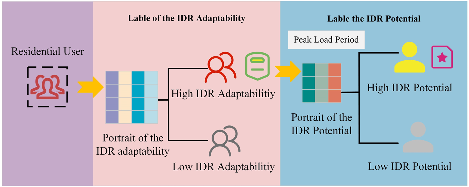
FIGURE 1. The labeling process of the graded user portrait.

3 The VAE-DBN based Load classification model considering the IDR adaptability and potential of the residential user

According to the labeling presented by Section 2.1.3 and Section 2.2.2, a number of samples in the load dataset can be labeled. Therefore, the labeled samples can be selected as the training dataset to train the VAE-DBN based classification model, which is able to implement the user classification for identifying the users with high IDR adaptabilities and potentials. As only a part of the samples is processed by the time-consuming labeling process, the rest samples are handled by the classification model automatically, thus the efficiency of the identification can be guaranteed.

3.1 VAE based load data pre-training model

The load data is normally with the characteristics of high dimension and long time period, which deteriorate the classification efficiency. In terms of improving the processing efficiency of the load data, this paper employs VAE to pre-train the input load data samples (Gunduz, 2021; Kingma, D.P., and Welling, M., 2014) to implement dimension reduction. VAE mainly consists of encoder, latent space, and decoder. The encoder maps high-dimensional data features to low-dimensional data features with specific distribution. The decoder receives the low-dimensional data features. And then, it carries out the sampling to reconstruct the high-dimensional data features.

In the training of the VAE model, firstly the encoder extracts the probability distribution $P_{\vartheta }\left(X\right)$ of the high-dimensional spatial features from the original load data X to achieve the distribution of latent variable $P_{\vartheta }\left(Z|X\right)$. $\vartheta$ is the network parameter. Using the mean $\mu$ and variance $\sigma$ of a given Z distribution, the original X can be mapped to an interval represented by the distribution $N\left(\mu ,\sigma \right)$. And then, the latent variable Z (lower-dimensional space) can be achieved based on the sampling of the interval. Finally, the decoder recovers the reconstructed $X^{\prime }$ which is approximate to the original X. Therefore, the encoding of the original load data X can be obtained in the lower-dimensional space. Figure 2 shows the structure of VAE model. And the brief introduction of VAE is also listed below.

1) Encoder introduces a posterior distribution $Q_{\varpi }\left(Z|X\right)$, which is an approximate inference of the posterior distribution of the latent variable Z. $\varpi$ is the network parameter. The target of the approximate inference is a normal distribution $N\left(\mu ,\sigma \right)$. It can be deduced that the posterior distribution $Q_{\varpi }\left(Z|X\right)$ approximate follows the normal distribution. The encoder model can be formed by Eq. 18:$\varpi$

$Encoder\left(X\right)=Q_{\varpi }\left(Z|X\right)\sim N\left(\mu ,\sigma \right)(18)$

where $\mu$ and $\sigma$ represent the mean and variance corresponding to the probability distribution of X in the encoding process.

2) Latent space: The mean $\mu$ and variance $\sigma$ can be generated by the encoder. From the posterior distribution $Q_{\varpi }\left(Z|X\right)$, the latent variable Z is sampled and subsequently sent to the decoder network by using the reparameterization trick. The latent variable Z is calculated by Eq. 19:

$Z=\mu +\epsilon •\sigma (19)$

where $\epsilon$ is sampled from a standard normal distribution $N\left(\mathrm{0,1}\right)$.

3) Decoder estimates a posterior distribution $P_{\vartheta }\left(Z|X\right)$, which generates the probability distribution of the reconstructed data $X^{\prime }$ according to the latent variable Z. It can be deduced that the distribution of reconstructed data $X^{\prime }$ follows the posterior distribution $P_{\vartheta }\left(Z|X\right)$. The decoder model can be formed by Eq. 20.

$Decoder\left(Z\right)=P_{\vartheta }\left(Z|X\right)(20)$

4) Loss function: In order to minimize the difference of the distribution between $Q_{\varpi }\left(Z|X\right)$ and $P_{\vartheta }\left(X\right)$, and reduce the reconstruction loss, the loss function can be constructed by Eq. 21:

$LOSS=-KL\left(Q_{\varpi }\left(Z|X\right)\Vert P_{\vartheta }\left(Z\right)\right)+E_{Q_{\varpi }\left(Z|X\right)}\ln \left(P_{\vartheta }\left(X|Z\right)\right)(21)$

Where the first term is to measure the similarity between the distribution $Q_{\varpi }\left(Z|X\right)$ and $P_{\vartheta }\left(Z\right)$ by using the Kullback-Leibler Divergence; the second term is a likelihood of the original load data being reconstructed (reconstruction term).

FIGURE 2

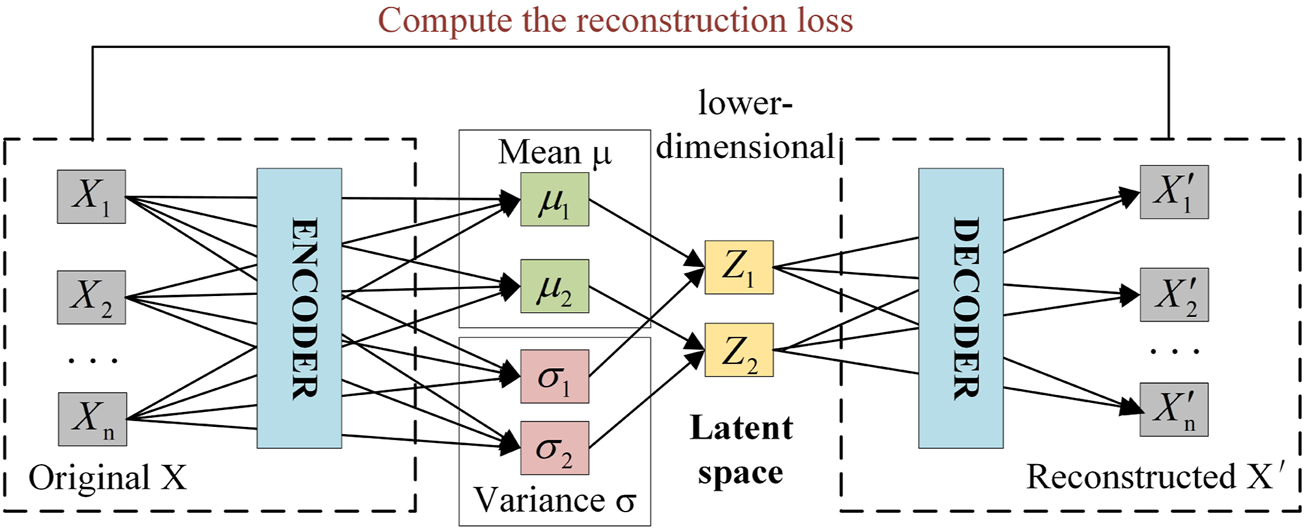
FIGURE 2. The structure of the VAE model.

After calculating $LOSS$ according to Eq. 21, the model parameters are optimized in the back propagation using the Adam optimizer. When the model converges, the training of the VAE model is completed. This process can affirm the dimension of the latent space to guarantee a lower reconstruction loss and preserve the original data characteristics.

3.2 DBN based Load Classification Model

DBN mainly consists of multiple restricted Boltzmann machines (RBM) (Lin et al., 2016). It is able to highlight the characteristic of the data, which is quite suitable for execute the classification task for the load data. RBM is a probabilistic modeling method based on the energy function. It consists of a hidden layer $\mathrm{h}=\left(h_1,h_2,h_3,\cdots h_{n_h}\right)$ and a visible layer$\mathrm{v}=\left(v_1,v_2,v_3,\cdots v_{n_v}\right)$. The weight matrix ${\mathrm{W}}_{n\times m}$ connects the layers to implement the bi-directional full connections. The structure of an RBM is shown in Figure 3.

FIGURE 3

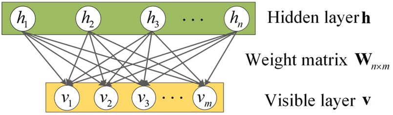
FIGURE 3. The structure of RBM.

For a given group of states $\left(\mathrm{v},\mathrm{h}\right)$, the joint probability energy function of the hidden layer and visible layer can be represented by Eq. 22:

$EF\left(\mathbf{v},\mathbf{h}\right)=-{\displaystyle \sum }_{i=1}^{n_v}{a}_i{v}_i-{\displaystyle \sum }_{j=1}^{n_h}{b}_j{h}_j-{\displaystyle \sum }_{i=1}^{n_v}{\displaystyle \sum }_{j=1}^{n_h}{h}_j{w}_{ji}{v}_i(22)$

Where $w_{ji}$ denotes the weight between the visible unit $v_i$ and the hidden unit $h_j$; $a_i$ represents the bias of the ith neuron in the visible layer; $b_j$ represents the bias of the jth neuron in the hidden layer; $n_v$ represents the number of the visible units; $n_h$ represents the number of the hidden units.

For any group status $\left(\mathrm{v},\mathrm{h}\right)$, the joint probability distribution can be represented by Eq. 23:

$P\left(\mathbf{v},\mathbf{h}\right)=e^{-EF\left(\mathbf{v},\mathbf{h}\right)}/{\displaystyle \sum }_{\mathbf{v},\mathbf{h}}{e}^{-EF\left(\mathbf{v},\mathbf{h}\right)}(23)$

If the visible states v is given, the activation probability for the hidden states h can be represented by Eq. 24:

$P\left(\mathbf{h}|\mathbf{v}\right)=S\left({\displaystyle \sum }_j^{n_v}{w}_{ji}^{\mathrm{T}}{h}_j+a_i\right)(24)$

If the hidden states h is given, the activation probability for the visible states v can be represented by Eq. 25:

$P\left(\mathbf{v}|\mathbf{h}\right)=S\left({\displaystyle \sum }_i^{n_h}{w}_{ji}^{\mathrm{T}}{v}_i+b_j\right)(25)$

In Eqs 24, 25, S represents the sigmoid activation function which is represented by Eq. 26:

$S\left(x\right)=1/\left(1+e^{-x}\right)(26)$

In terms of training the RBM, the tuning of the parameters is based on the maximization of the log likelihood of the training data. The partial derivative of the weight $w_{ji}$ can be computed using Eq. 27:

$\frac{\partial \ln \left(P\left(\mathbf{v}\right)\right)}{\partial w_{ji}}={\left[{\mathit{v}}_{\mathrm{i}}{\mathit{h}}_j\right]}_{\mathrm{D}}-{\left[v_i{h}_j\right]}_{\mathrm{M}}(27)$

Where ${\left[v_i{h}_j\right]}_{\mathrm{D}}$ and ${\left[v_i{h}_j\right]}_{\mathrm{M}}$ represent the expectations of the practical data distribution and the model distribution, respectively.

Due to the complexity and computational intensity of computing ${\left[v_i{h}_j\right]}_{\mathrm{M}}$, the contrastive divergence is adopted to estimate the gradient and moreover to update the weight ${\widehat{w}}_{ji}$ using Eq. 28:

${\widehat{w}}_{ji}=\eta \left({\left[v_i{h}_j\right]}_{\mathrm{D}}-{\left[v_i{h}_j\right]}_{\mathrm{r}\mathrm{e}}\right)(28)$

Where $\eta$ is the learning rate; ${\left[v_i{h}_j\right]}_{\mathrm{r}\mathrm{e}}$ is the distribution expectation reconstructed by the visible layer. Additionally, the biases $a_i$ and $b_j$ can be updated similarly.

During the training of the DBN classification model. The output of the last RBM is the input of the next RBM using the feed forward. And then, the supervised learning based back propagation is executed to adjust the parameters. This paper employs soft max to tune the parameters of DBN.

3.3 The detailed steps of training and classifying using VAE-DBN

Step.1: Data normalization. For a load dataset $X=\left\{X_1,\cdots ,X_{\mathbb{N}}\right\}$ composed of $\mathbb{N}$ samples of users, it is initially normalized to make the training process converge as soon as possible. The min-max normalization method is adopted, which is expressed as $X_{\mathrm{n}\mathrm{o}\mathrm{r}\mathrm{m}}=\left(X_{\mathrm{a}\mathrm{c}\mathrm{t}\mathrm{u}\mathrm{a}\mathrm{l}}-X_{\min }\right)/\left(X_{\max }-X_{\min }\right)$. $X_{\max }$, $X_{\min }$, $X_{\mathrm{a}\mathrm{c}\mathrm{t}\mathrm{u}\mathrm{a}\mathrm{l}}$, and $X_{\mathrm{n}\mathrm{o}\mathrm{r}\mathrm{m}}$ represents the maximum, minimum, actual, and norm value of the load data, respectively.

Step 2: Training VAE model. The normalized dataset $X_{\mathrm{n}\mathrm{o}\mathrm{r}\mathrm{m}}$ is input into the VAE model. And this model can be trained according to Eqs 18–21. Therefore, based on the VAE model, the lower-dimensional data $Z$ can be obtained from the encoder encoding $X_{\mathrm{n}\mathrm{o}\mathrm{r}\mathrm{m}}$ by Eq. 19. Subsequently, the decoder can reconstruct the load data $X_{\mathrm{n}\mathrm{o}\mathrm{r}\mathrm{m}}^{\prime }$ according to Eq. 20. Finally, the loss function $LOSS$ is utilized to optimize the parameter of the VAE model according to Eq. 21, until the model is converged.

Step 3: Training DBN model. The lower-dimensional data Z and their labels are input into the DBN model. At the outset of DBN model training, all parameters of the model are initialized. And then, each RBMs layer of the DBN model is trained according to Eqs 22–27 until the training of all RBMs is completed. The weight $w_{ji}$ of the RBMs layer can be updated by Eq. 28. At the end of the DBN model training, the soft max classifier is employed to optimize the weights and bias for each RBM of the DBN network. Up to this point, the VAE-DBN based classification model is completely trained and can be applied on classification.

Step 4: User classification. The presented user classifying process includes two classifying stages. In the first classification stage, the VAE-DBN model is applied to achieve the user classification for identifying the users with high IDR adaptabilities. The users with high IDR adaptabilities can be preliminarily selected and then proceed to the next classification stage. In the second classification stage, based on the load data of selected users in the peak load periods, the VAE-DBN model is applied to achieve the user classification for identifying the users with high IDR potentials.The process of the presented residential user portrait based VAE-DBN classification is shown in Figure 4.

FIGURE 4

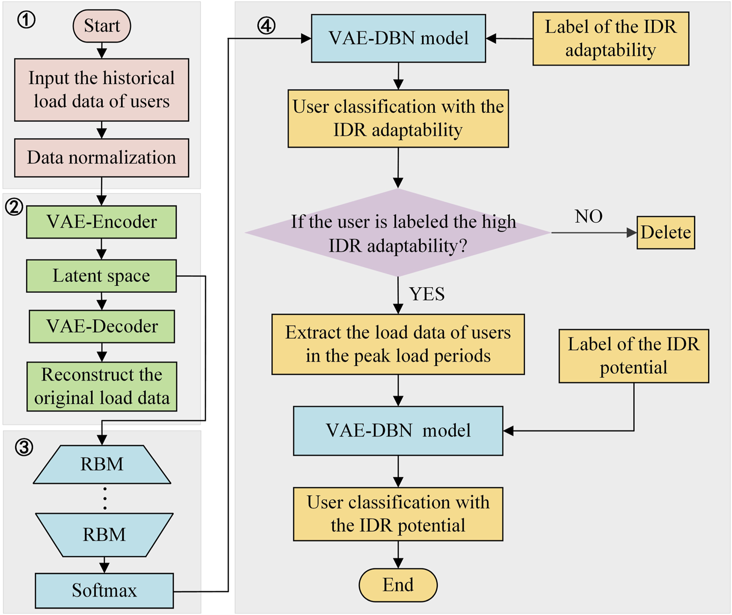
FIGURE 4. The detailed process of the VAE-DBN classification model.

4 Experimental result

The experiments are carried out using the computer with Inter(R) Core(TM) i5-1135G7 CPU 4.20GHz, RAM 16GB, OS Windows 11. In terms of highlighting the performance of the presented approaches, a synthesized load dataset based on the practical load is generated. The dataset contains 278 residential users. Each user contributes their daily load data for 91 days. The sampling interval of each daily load data is 15 min. Therefore, each sample of the load dataset is $4\times 24\times 91=8736$ dimensions. In the following experiments, if the experiments focus on studying the daily load, the sample with 8,736 dimensions will be converted into 91 daily load samples each of which is 96 dimensions. The experiments are mainly categorized into three types including the evaluation of the preliminary portrait of the IDR adaptability, the evaluation of the precise portrait of the IDR potential, and the evaluations of the VAE-DBN based load data classification.

4.1 Evaluation of IDR adaptability portrait and preliminary selection of IDR candidate users

4.1.1 Generation of typical daily load curve for user

Before generating the portraits of the residential users, as presented in Section 2.1.1, the typical daily load curve of each user should be extracted using the KANN-DBSCAN clustering algorithm. For each user, after processed by the clustering algorithm, the load samples are clustered into a number of clusters. And then, the centroid of the cluster which contains the greatest number of samples is selected as the typical daily load curve of the user. Figure 5 indicates the typical daily load curve for a user. It can be seen that a residential user clearly has various power consumption behaviors in different time periods, which potentially indicates that the user has potentials to participate in IDR. Moreover, the details of the centroid of the cluster selected for a user are listed in Table 3.

FIGURE 5

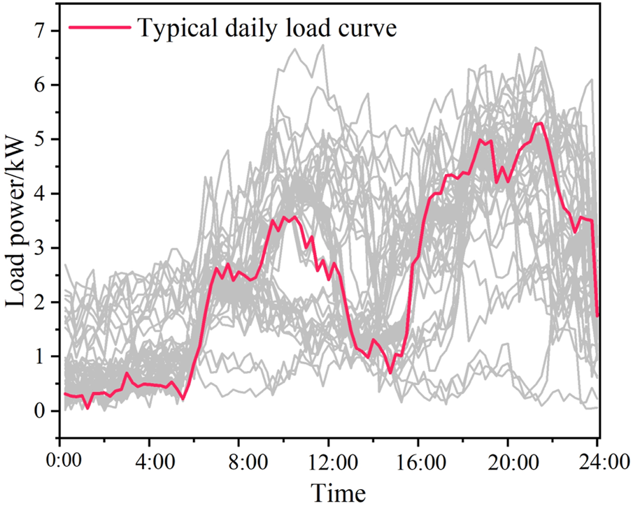
FIGURE 5. The typical daily load curve for a user in the load dataset.

TABLE 3

TABLE 3. The details of the centroid selected for a user in the load dataset.

Table 3 indicates the number of samples per cluster for a user in the load dataset. It is obvious that cluster 3 contains the largest number of samples. Therefore, the centroid of cluster 3 is extracted as a typical daily load curve for the user, which can be observed in Figure 5.

4.1.2 Portrait of the IDR adaptability and preliminary selection

Firstly, the responding willingness, power consumption regularity, power consumption volatility, and historical load level for each of the 278 users are computed according to the expressions listed in Table 1. Therefore, the portraits of the IDR adaptabilities of the 278 residential users can be generated. And then, the spectral clustering algorithm is applied on the portraits according to Algorithm 1. Based on Silhouette index (SI) and Davies Bouldin index (DBI), the optimal number of clusters of the users’ portraits can be identified (Wang et al., 2022). Figure 6 indicates the determination of the optimal cluster number for the portraits.

FIGURE 6

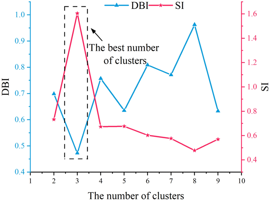
FIGURE 6. The determination of the optimal cluster number for the users’ portraits.

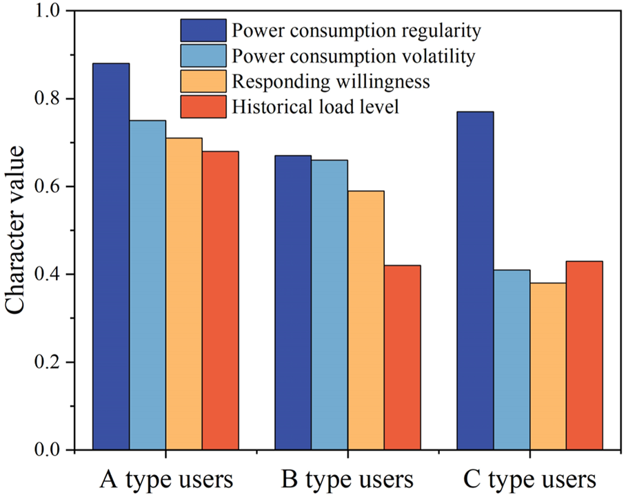
According to the improved entropy weight method presented in Section 2.1.3, the clusters of the portraits can be scored, and thus all the users in the corresponding clusters are scored. As the optimal cluster number is 3, three types of the scored users are finally identified. A type users are with high IDR adaptabilities; B type users are with medium IDR adaptabilities; C type users are with low IDR adaptabilities. The result is shown in Figure 7. Especially, the values of the responding willingness, power consumption regularity, power consumption volatility, and historical load level indicated in the figure are the average values of those of the users in the clusters.

FIGURE 7

FIGURE 7. Three types of the scored users with high, medium, and low IDR adaptabilities.

Figure 7 indicates that the responding willingness, power consumption regularity, power consumption volatility, and historical load level of the A type users show satisfied performance to participate in IDR. Therefore, in the practical IDR task, this kind of users can be firstly dispatched. B type users show weaker performance than that of A type users, which provides medium IDR adaptability. However, the figure indicates that if the responding willingness can be enhanced, for example based on the extra economic compensation, B type users are also valuable to participate in IDR. Although C type users show higher power consumption regularity, the other three indices are too low to be suitable for participating in the IDR tasks.

4.2 Evaluation of portrait of the IDR potential.

In this section, the peak period 1 (10:00–14:00) and peak period 2 (17:00–21:00) are employed to evaluate the effectiveness of the portrait of the IDR potential. Based on the preliminary selection of the users with high IDR adaptability, a number of 144 users belonged to A type are selected as the candidates. According to the presented portrait approach in Section 2.2, the portraits of the IDR potential for 144 users can be generated. And then, the spectral clustering algorithm and the improved entropy weight method are also applied to identify the users with different levels of IDR potentials. As a result, the type of high IDR potential users (Type III), the type of medium IDR potential users (Type II), and the type of low IDR potential users (Type I) can be achieved. The average IDR potential values of different user types in peak period 1 and peak period 2 are shown in Tables 4, 5. Both tables indicate the potential differences among different types of users.

TABLE 4

TABLE 4. Average values of different type IDR potential users in peak period 1.

TABLE 5

TABLE 5. Average values of different type IDR potential users in peak period 2.

In terms of indicating the performance of identifying users with different IDR potentials using the presented portrait approaches, the typical daily load curves of the users with different IDR potentials in peak period 1 are demonstrated in Figure 8.

FIGURE 8

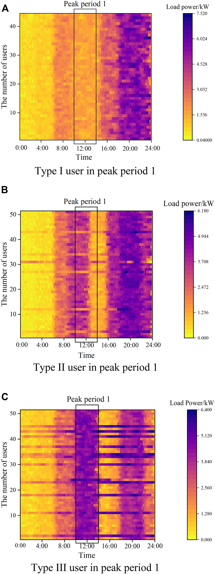
FIGURE 8. Typical load curves of users with different IDR potentials. (A) Type I user in peak period 1. (B) Type II user in peak period 1. (C) Type III user in peak period 1.

Figure 8 indicates that the portrait of the IDR potential is able to capture the overlapping between the peak period of user power consumption (dark area in the figure) and the peak load period of the system. According to three figures, Type III user has great potential to participate in IDR, which can contribute more to implement the load shifting.

Figure 9 uses a specific user as the example to show the portrait of the IDR adaptability and the portrait of the IDR potential.

FIGURE 9

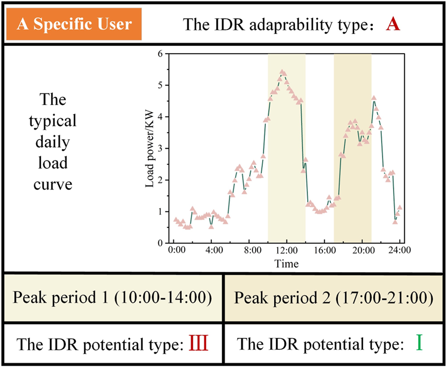
FIGURE 9. The portrait of the IDR adaptability and the portrait of the IDR potential for a specific user.

Figure 9 shows the typical daily load curve and the types of the IDR adaptability and the IDR potential of the specific user. The portraits can reflect the power consumption preference and if the user is suitable for participating IDR in certain periods. This figure indicates that the presented approaches of generating portraits can be suitable tools for the power company to select proper users to participate in IDR.

4.3 VAE-DBN based load classification

Based on the presented portraits and labeling approaches, the samples in the load dataset can be labeled. Therefore, the labeled samples can be regarded as the training samples to train the VAE-DBN classification model. And then, based on the trained classification model, the rest samples in the load dataset can be automatically and efficiently identified if they are suitable to participate in IDR. As a result, the efficiency of the identification can be guaranteed.

4.3.1 The parameters of the employed VAE-DBN

The load samples of the 278 residential users are divided into the training dataset containing 228 users and the testing dataset containing 50 users. The samples in both datasets are normalized and input into VAE-DBN to implement the training and testing respectively. The parameters employed by VAE-DBN are listed in Table 6.

TABLE 6

TABLE 6. The parameters employed by VAE-DBN.

4.3.2 The performance of the dimension reduction using VAE

The training dataset is employed to train VAE. The encoder of VAE inputs the training samples with 8,736 dimensions. Latent space outputs the dimension-reduced output with 20 dimensions. The decoder of VAE is to guarantee the dimension-reduced samples can also well represent the original data. Figure 10 shows the curve of the VAE reconstruction losses along with the increasing iterations.

FIGURE 10

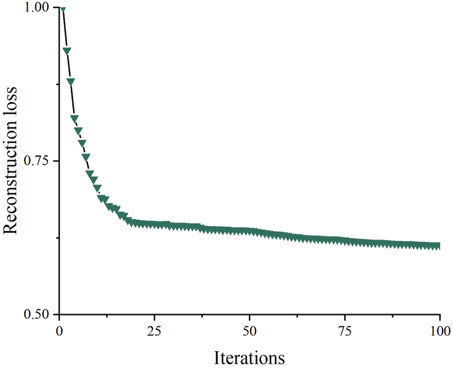
FIGURE 10. The curve of the training error of VAE.

The reduced dimension of VAE is based on the signal reconstruction loss and information retention rate of data under different data compression ratios (Wang et al., 2022). The reconstruction loss and the information retention rate can be computed by Eqs 29, 30:

${\epsilon }_e=\sqrt{\frac{{\displaystyle \sum }_{j=1}^m{\left(X_j-X_j^{\prime }\right)}^2}{m}}(29)$

${\pi }_r=1-\frac{{\displaystyle \sum }_{j=1}^{d_{en}}{\Vert X_j-X_j^{\prime }\Vert }^2/d_{en}}{{\displaystyle \sum }_{j=1}^m{\Vert X_j\Vert }^2/m}(30)$

Where X and$X^{\prime }$ represents the original data and the reconstructed data; m, $d_{en}$ denotes the dimension of the original data, the dimension of dimension-reduced output, respectively.

When the dimension is reduced from 8,736 to 20, the signal reconstruction loss ${\epsilon }_e$ is 0.84 and the information retention rate ${\pi }_r$ is 86%. When the dimension is reduced from 8,736 to 10, the signal reconstruction loss ${\epsilon }_e$ is 0.79 and the information retention rate ${\pi }_r$ is 79%. The above results suggest that although the high-dimensional load sample is significantly reduced, the data information of the original sample doesn’t lose too much. Benefitting from this point, the efficiency of the VAE dimension reduction based classification can be improved.

4.3.3 The performance of the classification using VAE

In terms of demonstrating the effectiveness of VAE-DBN, this section classifies the users according to their IDR adaptabilities and IDR potentials in peak period 1. In this case, the VAE dimension-reduced training samples are firstly input into DBN to implement the training. As long as the training phase finishes, the DBN can be employed to carry out the classification using the VAE dimension-reduced testing data samples. Additionally, in terms of further demonstrating the effectiveness of VAE, two widely used dimension reduction algorithms including PCA and auto encoder (AE) are also implemented. PCA is a linear transformation algorithm, which projects a high-dimensional data set into a new subspace where the orthogonal axes are located. However, the quality of dimensionality reduction cannot be guaranteed when the high-dimensional dataset does not present linear correlation. AE has nonlinear dimensionality reduction capability, which can learn high-dimensional data features to a lower dimension on the basis of supervised learning. Therefore, in order to evaluate the dimensionality reduction effect of different algorithms, the dimensionality of dimensionality reduction is uniformly set to 20.

The comparisons of the classification accuracy and efficiency are shown in Figure 11. In the figure, D represents the classification using the standard DBN without any dimension reduction; P-D represents the classification using the PCA based DBN; A-D represents the classification using the AE based DBN; V-D represents the classification using the presented VAE based DBN. In this paper, classification accuracy is used for measuring the correct classification performance of an algorithm, which can be calculated by dividing the number of correctly classified samples by the total number of samples.

FIGURE 11

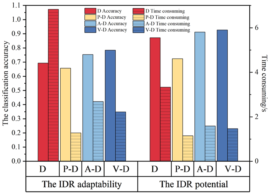
FIGURE 11. Comparison of classification using different dimension reduction algorithms based DBN.

Figure 11 indicates that VAE-DBN finds a compromise between the accuracy and efficiency. The algorithm can provide satisfied classification accuracy with high efficiency. Contrarily, although PCA based DBN outperforms the other algorithms in terms of efficiency, it shows the worst classification accuracy. The reason is that PCA depends on the linear correlation of the samples. However, the load sample is frequently nonlinear correlation. The figure also shows that AE based DBN can also provide similar performances compared to those of the VAE-DBN. However, the experiments suggest that VAE-DBN can more effectively learn the low dimensional representation of the sample data. Therefore, VAE-DBN still outperforms the AE based DBN.

In terms of comparison the performance of the classifiers, this paper also implements a number of popular classifiers including MLP, BPNN, K nearest neighbors (KNN). The comparison of the classification accuracy is shown in Figure 12. In the figure, V-M represents the classification using the VAE based MLP; V-B represents the classification using the VAE based BPNN; V-K represents the classification using the VAE based KNN; V-D represents the classification using the presented VAE based DBN.

FIGURE 12

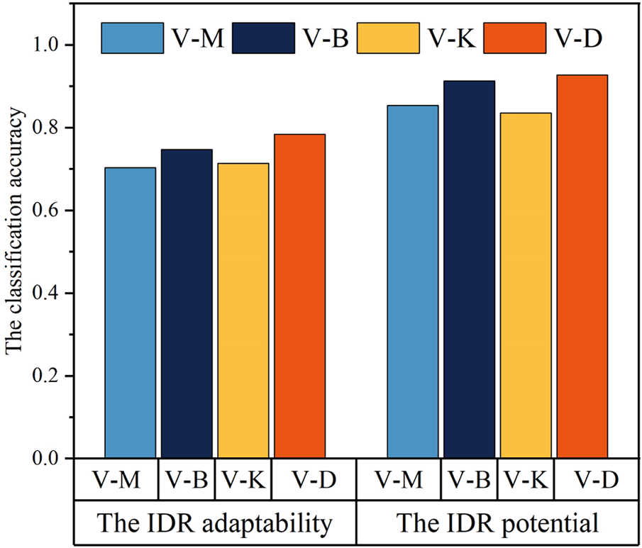
FIGURE 12. Comparison of classification using different classifiers with VAE.

Figure 12 shows that compared to the MLP and KNN, the supervised neural network algorithms perform higher accuracies. Especially, in both IDR adaptability and IDR potential classifications, DBN outperforms the other algorithms, which indicates that deep learning algorithm is able to precisely identify the hyperplane among classes, and thus it classifies the load data with satisfied accuracies.

Table 7 illustrates the comparison of the classification accuracy based on VAE-DBN with different dimensions. When the dimensionality rises to 20 dimensions, the classification accuracy has reached a relatively stable state. Thereafter, the classification accuracy doesn’t vary greatly with the increasing number of dimensions. This point is also the reason that why this paper finally employs 20-dimension to carry out the classification tasks.

TABLE 7

TABLE 7. The comparison of classification accuracy based on VAE-DBN with different dimensions.

For evaluating the training efficiencies of the VAE-DBN and the standard DBN classification models, the synthetic loaded dataset is duplicated from 16 to 512 MB. Table 8 demonstrates that the training times of both models increase when the volume of training data increases. Obviously, the training time of the VAE-DBN model does not increase sharply compared to that of the DBN model. The reason is that VAE-DBN converts the high-dimensional data into low-dimensional data to train the classification model, which greatly improves the training efficiency of VAE-DBN in the classification tasks.

TABLE 8

TABLE 8. Training efficiency comparison of VAE-DBN and DBN.

Figure 13 shows the efficiencies of the portrait of IDR potential based on the high IDR adaptability users, the classification using the standard DBN, and the classification using VAE-DBN. It can be seen from the figure that because of the overheads for computing multiple indices, the portrait is quite time consuming. Especially along with the increasing number of new users, the time of generating portraits increases sharply. Contrarily, the times of the classification based on standard DBN and VAE-DBN are relatively low. And benefiting from the dimension reduction, VAE-DBN outperforms DBN. This point significantly proves that, although the portrait is able to delineate the characteristics of the power consumption of the residential users, its efficiency is not quite satisfied. However, the portrait based labeling can help the deep learning algorithm be aware of the features of the users with high adaptabilities and potentials. As a result, the classification can significantly improve the efficiency for the power company to identify the valuable user to participate in IDR.

FIGURE 13

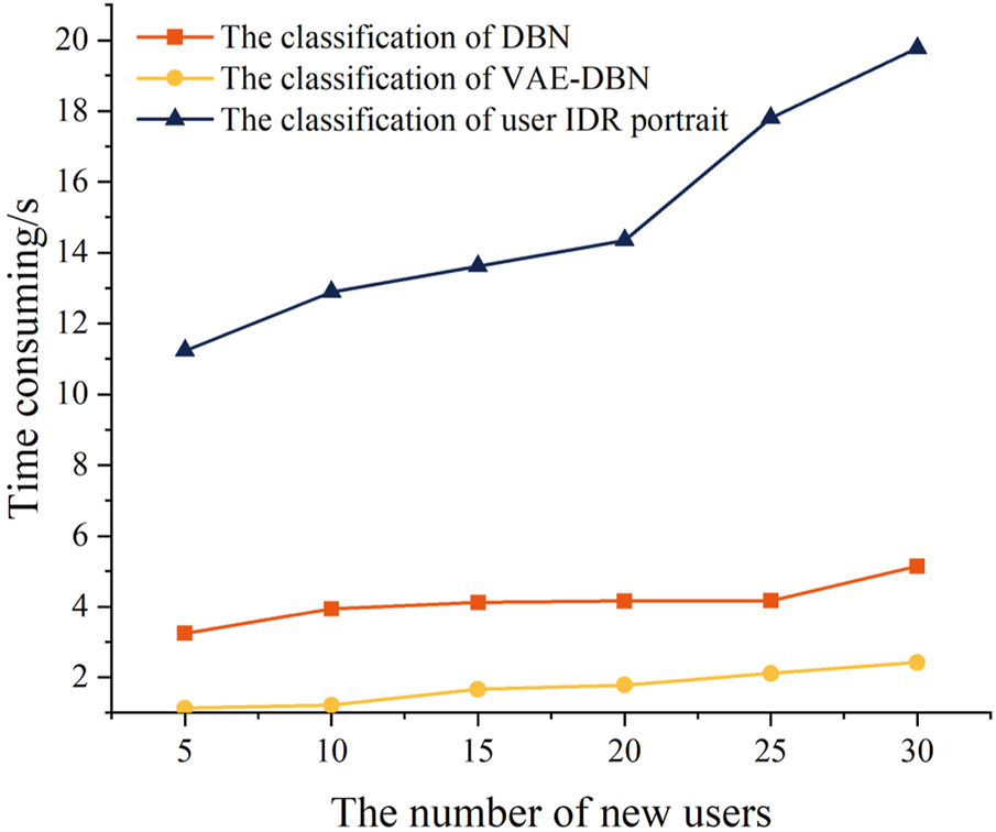
FIGURE 13. The algorithm efficiencies of the portrait and classification.

5 Conclusion

Currently, the portrait for the power consumption of the residential users and the load classification algorithms have less considerations for serving the identification of IDR participation. Therefore, this paper presents a residential user classification approach based on the graded user portrait with considering the IDR adaptability and the IDR potential. Based on the portrait of the IDR adaptability, the users with high adaptabilities can be preliminarily selected. And then, based on the portrait of the IDR potential, the users with high adaptabilities and potentials in different periods can be finally identified. Further, to solve the low efficiency issue of the portrait, the labeling based on the portrait is also presented. The labeling finally leads to the implementation of the VAE-DBN based user classification. VAE-DBN not only improves the efficiency of the user identification for participating in IDR, but also significantly reduces the dimension of the users’ samples, which also improves the efficiency of the classification. The experimental results suggest that the presented approaches can be effective tools for power company to identify suitable residential users to participate in IDR.

Data availability statement

The original contributions presented in the study are included in the article/Supplementary Material, further inquiries can be directed to the corresponding author.

Author contributions

YH and YL propose the idea of the study. YH, LX, and HG implement the algorithms and analyze the experimental results. All authors participate in the writing of the manuscript.

Conflict of interest

The authors declare that the research was conducted in the absence of any commercial or financial relationships that could be construed as a potential conflict of interest.

Publisher’s note

All claims expressed in this article are solely those of the authors and do not necessarily represent those of their affiliated organizations, or those of the publisher, the editors and the reviewers. Any product that may be evaluated in this article, or claim that may be made by its manufacturer, is not guaranteed or endorsed by the publisher.

Supplementary material

The Supplementary Material for this article can be found online at: https://www.frontiersin.org/articles/10.3389/fenrg.2022.1012721/full#supplementary-material

References

Agiollo, A., and Omicini, A. (2021). Load classification: A case study for applying neural networks in hyper-constrained embedded devices. Appl. Sci. (Basel). 11 (24), 11957. doi:10.3390/app112411957

CrossRef Full Text | Google Scholar

Ahir, R. K., and Chakraborty, B. (2022). A novel cluster-specific analysis framework for demand-side management and net metering using smart meter data. Sustain. Energy Grids Netw. 31, 100771. doi:10.1016/J.SEGAN.2022.100771

CrossRef Full Text | Google Scholar

Alrumayh, O., and Bhattacharya, K. (2019). Flexibility of residential loads for demand response provisions in smart grid. IEEE Trans. Smart Grid 10 (6), 6284–6297. doi:10.1109/TSG.2019.2901191

CrossRef Full Text | Google Scholar

Anowar, F., Sadaoui, S., and Selim, B. (2021). Conceptual and empirical comparison of dimensionality reduction algorithms (PCA, KPCA, LDA, MDS, SVD, LLE, ISOMAP, LE, ICA, t-SNE). Comput. Sci. Rev. 40, 100378. doi:10.1016/j.cosrev.2021.100378

CrossRef Full Text | Google Scholar

Arvanitidis, A. I., Bargiotas, D., Daskalopulu, A., Kontogiannis, D., Panapakidis, I. P., and Tsoukalas, L. H. (2022). Clustering informed MLP models for fast and accurate short-term load forecasting. Energies 15 (4). doi:10.3390/en15041295

CrossRef Full Text | Google Scholar

Asadinejad, A., Tomsovic, K., and Chen, C. F. (2017). Impact of residential customer classification on demand response results under high renewable penetration. Chicago, IL, USA: IEEE Power & Energy Society General Meeting PESGM. doi:10.1109/PESGM.2017.8274062

CrossRef Full Text | Google Scholar

Assad, U., Hassan, M. A. S., Farooq, U., Kabir, A., Khan, M. Z., Bukhari, S. S. H., et al. (2022). Smart grid, demand response and optimization: A critical review of computational methods. Energies 15 (6), 2003. doi:10.3390/EN15062003

CrossRef Full Text | Google Scholar

Chen, W. H., Xu, Y. H., Yu, Z. W., Cao, W. M., Chen, L., and Han, G. (2020). Hybrid dimensionality reduction forest with pruning for high-dimensional data classification. IEEE Access 8, 40138–40150. doi:10.1109/ACCESS.2020.2975905

CrossRef Full Text | Google Scholar

Chen, X., Yang, Y., Liu, Y., and Wu, L. (2021). Feature-driven economic improvement for network-constrained unit commitment: A closed-loop predict-and-optimize framework. IEEE Trans. Power Syst. 37 (4), 3104–3118. doi:10.1109/TPWRS.2021.3128485

CrossRef Full Text | Google Scholar

Chen, Y. Q., Zhao, B. N., Chen, C., Zhao, B. B., and Zhao, P. D. (2022). Identification of ore-finding targets using the anomaly components of ore-forming element associations extracted by SVD and PCA in the Jiaodong gold cluster area, Eastern China. Ore Geol. Rev. 144. doi:10.1016/j.oregeorev.2022.104866

CrossRef Full Text | Google Scholar

ChenGao, C. P. H., Jiang, J. G., Wang, H., Li, P., and Wan, S. H. (2021). A deep learning based non-intrusive household load identification for smart grid in China. Comput. Commun. 177, 176–184. doi:10.1016/J.COMCOM.2021.06.023

CrossRef Full Text | Google Scholar

Dai, X. J., and Zeng, Z. C. (2022). Research on spectral clustering algorithm for network communication big data based on wavelet analysis. Int. J. Auton. Adapt. Commun. Syst. 15 (2), 93–105. doi:10.1504/IJAACS.2022.123459

CrossRef Full Text | Google Scholar

Ebrahimi, S., Kinnon, M., and Brouwer, J. (2018). California end-use electrification impacts on carbon neutrality and clean air. Appl. Energy 213, 435–449. doi:10.1016/j.apenergy.2018.01.050

CrossRef Full Text | Google Scholar

Gaba, M., and Chanana, S. (2021). A non-cooperative game based energy management considering distributed energy resources in price-based and incentive-based demand response program. Int. J. Emerg. Electr. Power Syst. 22 (6), 807–830. doi:10.1515/ijeeps-2021-0021

CrossRef Full Text | Google Scholar

Guan, W. L., Zhang, D. L., Yu, H., Peng, B. G., Wu, Y. F., Yu, T., et al. (2021). Customer load forecasting method based on the industry electricity consumption behavior portrait. Front. Energy Res. 9. doi:10.3389/FENRG.2021.742993

CrossRef Full Text | Google Scholar

Gunduz, H (2021). An efficient dimensionality reduction method using filter-based feature selection and variational autoencoders on Parkinson's disease classification. Biomed. Signal Process. Control 66, 102452. doi:10.1016/j.bspc.2021.102452

CrossRef Full Text | Google Scholar

Huang, L., Chen, S. J., Ling, Z. X., Cui, Y. B., and Wang, Q. (2021). Non-invasive load identification based on LSTM-BP neural network. Energy Rep. 7 (S1), 485–492. doi:10.1016/j.egyr.2021.01.040

CrossRef Full Text | Google Scholar

Jiang, W., Pan, X., Jiang, K., Wen, L., and Dong, Q. (2018). Energy-aware design of stochastic applications with statistical deadline and reliability guarantees. IEEE Trans. Comput. -Aided. Des. Integr. Circuits Syst. 38 (8), 1413–1426. doi:10.1109/TCAD.2018.2846652

CrossRef Full Text | Google Scholar

Jing, Y., and Ying, T. (2019). An intelligent fault diagnosis method using GRU neural network towards sequential data in dynamic processes. Processes 7 (3), 152. doi:10.3390/pr7030152

CrossRef Full Text | Google Scholar

Kingma, D. P., and Welling, M. (2014). Auto-encoding variational bayes. arXiv.org

Google Scholar

Laitsos, V. M., Bargiotas, D., Daskalopulu, A., Arvanitidis, A. I., and Tsoukalas, L. H. (2021). An incentive-based implementation of demand side management in power systems. Energies 14 (23). doi:10.3390/EN14237994

CrossRef Full Text | Google Scholar

Lee, E., Kim, J., and Jang, D. (2020). Load profile segmentation for effective residential demand response program: Method and evidence from Korean pilot study. Energies 13, 1348. doi:10.3390/en13061348

CrossRef Full Text | Google Scholar

Li, S. Q., Xu, Q., Liu, J. L., Shen, L. Y., and Chen, J. D. (2022). Experience learning from low-carbon pilot provinces in China: Pathways towards carbon neutrality. Energy Strategy Rev. 42, 100888. doi:10.1016/J.ESR.2022.100888

CrossRef Full Text | Google Scholar

Li, W. J., Yan, S. Q., Jiang, Y., Zhang, S. Z., and Wang, C. L. (2019). Research on method of self-adaptive determination of DBSCAN algorithm parameters. Comput. Eng. Appl. 55 (5), 1–7+148. doi:10.3778/j.issn.1002-8331.1809-0018

CrossRef Full Text | Google Scholar

Li, Y. J., and Chen, L. J. (2020). Improved LSTM data analysis system for IoT-based smart classroom. J. Intelligent Fuzzy Syst. 39 (4), 5141–5148. doi:10.3233/JIFS-179999

CrossRef Full Text | Google Scholar

Liang, H. S., and Ma, J. (2021). Develop load shape dictionary through efficient clustering based on elastic dissimilarity measure. IEEE Trans. Smart Grid 12 (1), 442–452. doi:10.1109/TSG.2020.3017777

CrossRef Full Text | Google Scholar

Lin, E., Mukherjee, S., and Kannan, S. (2020). A deep adversarial variational autoencoder model for dimensionality reduction in single-cell RNA sequencing analysis. BMC Bioinforma. 21 (64). doi:10.1186/s12859-020-3401-5

PubMed Abstract | CrossRef Full Text | Google Scholar

Lin, P., Fu, S., Wang, S., Lai, Y., and Tsao, Y. (2016). Maximum entropy learning with deep belief networks. Entropy 18 (251). doi:10.3390/e18070251

CrossRef Full Text | Google Scholar

Liu, Y., Li, X., Chen, X. B., Wang, X., and Li, H. Q. (2020). High-performance machine learning for large-scale data classification considering class imbalance. Sci. Program. 2020, 1–16. doi:10.1155/2020/1953461

CrossRef Full Text | Google Scholar

Lu, X., Xu, C. L., Leng, Z. Y., Wu, H. W., and Chen, Z. (2021). Load characteristic portrait model of power users in epidemic stage applying data-driven method. Electr. Power Constr. 42 (2), 93–106. doi:10.12204/j.issn.1000-7229.2021.02.012

CrossRef Full Text | Google Scholar

Paul, R., and Chalup, S. K. (2017). A study on validating non-linear dimensionality reduction using persistent homology. Pattern Recognit. Lett. 100, 160–166. doi:10.1016/j.patrec.2017.09.032

CrossRef Full Text | Google Scholar

Phyo, P. P., and Jeenanunta, C. (2021). Daily load forecasting based on a combination of classification and regression tree and deep belief network. IEEE Access 9, 152226–152242. doi:10.1109/ACCESS.2021.3127211

CrossRef Full Text | Google Scholar

Qi, N., Cheng, L., XuWang, H. L. Z. H., and Zhou, X. Y. (2020). Practical demand response potential evaluation of air-conditioning loads for aggregated customers. Energy Rep. 6 (S9), 71–81. doi:10.1016/J.EGYR.2020.12.019

CrossRef Full Text | Google Scholar

Ray, P., Reddy, S. S., and Banerjee, T. (2021). Various dimension reduction techniques for high dimensional data analysis: A review. Artif. Intell. Rev. 54 (5), 3473–3515. doi:10.1007/s10462-020-09928-0

CrossRef Full Text | Google Scholar

Sandels, C., Kempe, M., Brolin, M., and Mannikoff, A. (2019). Clustering residential customers with smart meter data using a data analytic approach - external validation and robustness analysis. In International conference on power and energy systems. Perth, WA, Australia: ICPES. doi:10.1109/ICPES47639.2019.9105484

CrossRef Full Text | Google Scholar

Song, J. Y., Cui, Y. W., Li, X. R., Zhong, W., Zou, X., and Li, P. Q. (2020). Load curve clustering method based on euclidean dynamic time warping distance and entropy weight. Automation Electr. Power Syst. 44 (15), 87–94. doi:10.7500/AEPS20191016008

CrossRef Full Text | Google Scholar

Song, Z. F., Shi, J., Li, S. J., Chen, Z. X., Yang, W. W., and Zhang, Z. T. (2020). Day ahead bidding of a load aggregator considering residential consumers demand response uncertainty modeling. Appl. Sci. 10 (20), 7310. doi:10.3390/app10207310

CrossRef Full Text | Google Scholar

Srivastava, P. R., Sarkar, P., and Hanasusanto, G. A. (2022). A robust spectral clustering algorithm for sub-Gaussian mixture models with outliers. Operations Res. doi:10.1287/opre.2022.2317

CrossRef Full Text | Google Scholar

Vahedipour-Dahraie, M., Rashidizadeh-Kermani, H., Anvari-Moghaddam, A., Siano, P., and Catalao, J. P. S. (2022). Short-term reliability and economic evaluation of resilient microgrids under incentive-based demand response programs. Int. J. Electr. Power & Energy Syst. 138, 107918. doi:10.1016/J.IJEPES.2021.107918

CrossRef Full Text | Google Scholar

Wan, Q. Z., and Yu, Y. (2020). Power load pattern recognition algorithm based on characteristic index dimension reduction and improved entropy weight method. Energy Rep. 6 (S9), 797–806. doi:10.1016/J.EGYR.2020.11.129

CrossRef Full Text | Google Scholar

Wang, H. X., Yuan, J. H., Qi, G. Q., Li, Y. Z., Yang, J. Y., Dong, H. N., et al. (2021). A data-driven load forecasting method for incentive demand response. Energy Rep. 8 (S4), 1013–1019. doi:10.1016/j.egyr.2022.01.232

CrossRef Full Text | Google Scholar

Wang, L., Liu, Y., Li, W., Zhang, J., Xu, L., and Xing, Z. (2022). Two-stage power user classification method based on digital feature. Portraits Power Consum. Behav. Electr. Power Constr. 43 (2). doi:10.12204/j.issn.1000-7229.2022.02.009

CrossRef Full Text | Google Scholar

WangYang, Y. W., Xiao, X., and Zhang, X. (2022). Clustering and analysis of electricity consumption behavior of massive users based on network feature dimension reduction of denoising autoencoder and improved mini-batch K-means algorithm. Electr. Power Autom. Equip. 42 (6). doi:10.16081/j.epae.202203017

CrossRef Full Text | Google Scholar

Wei, Y., Levesque, J. P., Hansen, C. J., Mauel, M. E., and Navratil, G. A. (2021). A dimensionality reduction algorithm for mapping tokamak operational regimes using a variational autoencoder (VAE) neural network. Nucl. Fusion 61 (12), 126063. doi:10.1088/1741-4326/ac3296

CrossRef Full Text | Google Scholar

Weitzel, T., and Glock, C. H. (2019). Scheduling a storage-augmented discrete production facility under incentive-based demand response. Int. J. Prod. Res. 57 (1), 250–270. doi:10.1080/00207543.2018.1475764

CrossRef Full Text | Google Scholar

Wu, D., Wang, Y. C., Li, L., Lu, P. F., Liu, S. Y., Dai, C., et al. (2022). Demand response ability evaluation based on seasonal and trend decomposition using LOESS and S–G filtering algorithms. Energy Rep. 8 (S5), 292–299. doi:10.1016/J.EGYR.2022.02.139

CrossRef Full Text | Google Scholar

Xu, M. J., and Wang, Y. H. (2017). Residential electricity consumption behavior mining based on system cluster and grey relational degree. Energy Power Eng. 9 (4), 390–400. doi:10.4236/epe.2017.94b044

CrossRef Full Text | Google Scholar

Yin, H. L., Zhang, X. W., Wang, F. D., Zhang, Y. N., Xia, R. L., and Jin, J. (2021). Rainfall-runoff modeling using LSTM-based multi-state-vector sequence-to-sequence model. J. Hydrology 598, 126378. doi:10.1016/j.jhydrol.2021.126378

CrossRef Full Text | Google Scholar

Yoshida, A., Manomivibool, J., Tasaki, T., and Unroj, P. (2020). Qualitative study on electricity consumption of urban and rural households in chiang rai, Thailand, with a focus on ownership and use of air conditioners. Sustainability 12, 5796. doi:10.3390/su12145796

CrossRef Full Text | Google Scholar

Zhang, Y. M., Han, X. S., Yang, M., Xu, B., Zhao, Y. C., and Zhai, H. F. (2018). Adaptive robust unit commitment considering distributional uncertainty. Int. J. Electr. Power & Energy Syst. 104, 635–644. doi:10.1016/j.ijepes.2018.07.048

CrossRef Full Text | Google Scholar

Zhou, K. L., Yang, S. L., and Shen, C. (2013). A review of electric load classification in smart grid environment. Renew. Sustain. Energy Rev. 24, 103–110. doi:10.1016/j.rser.2013.03.023

CrossRef Full Text | Google Scholar

Zhu, H. X., Wang, Q., Li, C. C., and Yu, C. (2020). Electricity safety analysis and improvement based on user classification. 2020 international conference on energy, environment and engineering (ICEEB 2020), xi'an. China. doi:10.1051/e3sconf/202018501025

CrossRef Full Text | Google Scholar