CEEMDAN-CatBoost-SATCN-based short-term load forecasting model considering time series decomposition and feature selection

1 Introduction

Aiming for carbon neutrality, developing distributed renewable energy-dominated energy systems has become an inexorable trend (Rehman et al., 2021; Li C et al., 2022). Together with the proliferation of electric vehicles and energy storage systems, this development trend has considerably increased the randomness and uncertainty of electrical loads, which has greatly increased the difficulty of short-term load forecasting (Deng et al., 2022). Therefore, developing accurate, fast, and effective short-term load forecasting methods has become an urgent demand for adapting to changes and promoting the development of emerging power systems.

Traditional machine learning methods represented by extreme learning machine (ELM), support vector machine (SVM), BP neural network, and random forest (RF) have been widely used in short-term load forecasting (Aasim et al., 2021; Huang et al., 2021; Xiao et al., 2022). With the rapid development of deep learning in the fields of computer vision, natural language processing, and speech recognition, recurrent neural networks represented by long short-term memory (LSTM) neural networks have been applied in the field of electrical load forecasting (Tan et al., 2020; Ge et al., 2021; Li S et al., 2022). Through time series modeling, electrical load statues over a period of time can be effectively perceived, achieving accurate identification of short-term load fluctuation patterns and long-term load change trends. However, when dealing with the input of an increasingly lengthening load time series, the dimension of the input layer, the number of layers, and the neurons of each layer continue to grow, resulting in difficulties in the training process and the issue of slow convergence. Based on the idea of time series modeling, the convolutional neural network (CNN) can be transformed into the temporal convolutional network (TCN) by making a node in the current layer which no longer depends on nodes that represent the previous time steps in the same layer but depends on those in the previous layer representing the previous time steps. This enables parallelizing the computing tasks of nodes that represent different time steps in the same layer. Independent parallel computing of large-scale convolution kernels can be realized, and the aforementioned problems can be effectively avoided (Luo et al., 2021). Hu et al. (2022) propose a quantile regression-integrated TCN to conduct electrical load forecasting. This model uses intervals to describe the probability distribution of future loads. Considering the influencing factors of load forecasting, Bian et al. (2022) use the temporal convolutional network to extract the potential association between time series data and non-time series data, then build time series features, and finally output the best load forecasts. Zhu et al. (2020) forecast the wind power output with the temporal convolutional network and compare the performance of LSTM and GRU. The result shows a higher forecasting accuracy of TCN.

Considering that various periodic fluctuation components hide in the original customer electrical load curves, time series decomposition methods such as empirical mode decomposition (EMD) and variational mode decomposition (VMD) can effectively help improve the accuracy of short-term load forecasting (Bedi and Toshniwal, 2018; Ye et al., 2022). However, some intrinsic mode components obtained by decomposition may have similar frequencies and fluctuation patterns. Exhaustively processing them all may result in an extra computational burden. Compared with the aforementioned methods, CEEMDAN can effectively improve the decomposition efficiency by adding auxiliary white noise to the original signal and solve the problems of a large reconstruction error and poor decomposition integrity of traditional methods (Zhang et al., 2017; Zhou et al., 2019). There are a lot of possible influencing factors to short-term load forecasting, but many of them are in fact redundant and irrelevant. Filter-based feature selection methods, such as those based on minimal redundancy maximal relevance (mRMR), can effectively reduce the feature dimension (Duygu, 2020; Yuan and Che, 2022) and thereby improve the efficiency of the subsequent training tasks. However, the mainstream filter-based feature selection methods merely assess the effect of individual features but are unable to assess the comprehensive performance of feature subsets. However, the CatBoost model uses combined category features to make use of the relationship between features, which greatly enriches feature dimensions, and it can realize the selection of the optimal feature set (Hancock and Khoshgoftaar, 2020; Mangalathu et al., 2020).

To this end, based on complete ensemble empirical mode decomposition with adaptive noise (CEEMDAN), CatBoost, and SATCN, this paper proposes a short-term load forecasting model. The original load time series is first decomposed into several intrinsic mode function (IMF) components and a residual with CEEMDAN. Then, permutation entropy values of them are calculated to determine which components should be merged for balancing the forecasting accuracy and the computational efficiency. The CatBoost-based recursive feature reduction method is applied to optimize the input feature set of individual components. A self-attention mechanism-integrated temporal convolutional network (SATCN) model that integrates CNN and the self-attention mechanism is then trained to output forecasts corresponding to the components. At last, the forecasts are combined to generate the short-term load forecast.

2 Decomposition of the load time series

2.1 Complete ensemble empirical mode decomposition with adaptive noise

CEEMDAN obtains IMF components by adding multiple adaptive Gaussian white noise sequences and averaging the decomposition results from EMD. The unique residual calculation method of CEEMDAN endows integrity to the decomposition process, which not only mitigates the inherent mode-mixing phenomenon of the existing EMD but also considerably reduces the signal reconstruction error, making the reconstructed signal almost identical to the original one (Chen et al., 2021).

This paper uses $L\left(t\right)$ to denote the original load time series. $E_i\left(\cdot \right)$ represents the ith IMF component obtained by EMD. $W_i\left(t\right)$ denotes the ith Gaussian white noise sequence that has the same length as $L\left(t\right)$. At the kth CEEMDAN decomposition stage, the amplitude coefficient of $w_i\left(t\right)$ is set at ${\epsilon }_k$. ${\overline{I}}_{k+1}$ is the k+1th CEEMDAN IMF component.

The steps of the CEEMDAN algorithm are as follows:

2.2 Permutation entropy of the load time series

The complexity of a time series can be measured by the time series permutation entropy (Zhao et al., 2022), which will be used as the basis for component merger and reorganization. For enough a number of components, when their permutation entropy values are close, the correspondingly indicated fluctuation patterns of the load time series are similar. Therefore, these components can be merged and reorganized to reduce the computational burden for the subsequent forecasting task. Considering a one-dimensional load time series $x^{Load}=\left\{x_1^L,x_2^L,\cdot \cdot \cdot ,x_N^L\right\}$, it can be reconstructed into a two-dimensional matrix $X^{Load}$ as in Eq. 7, where R represents the number of samples of row vectors and $\tau$ represents the sampling interval.

$X^{Load}=\left\{\begin{array}{llll}{x}_1^L& x_{1+\tau }^L& \cdots & x_{1+\left(R-1\right)\times \tau }^L\\ x_2^L& x_{2+\tau }^L& \cdots & x_{2+\left(R-1\right)\times \tau }^L\\ \cdots & \cdots & \cdots & \cdots \\ x_{N-\left(R-1\right)\times \tau }^L& x_{N-R\times \tau }^L& \cdots & x_N^L\end{array}\right\}.(7)$

This paper first sorts the reconstructed row vectors in $X^{Load}$ in descending order, and the column indices of the elements are written in a sorted row vector i as $\left\{\left(i,j_1\right),\left(i,j_2\right),\cdots ,\left(i,j_L\right)\right\}$, where $X_{i,j_1}^L\ge X_{i,j_2}^L\ge \cdots \ge X_{i,j_L}^L$ and L represents the length of the sampling dimension. It is worthwhile to mention that when two compared elements in a row vector have the same value, the one with the larger column index is sorted in the front.

For any row vector $X_i^{Load}$, a corresponding load fluctuation pattern can be defined with the column index sequence after being sorted. This paper uses $S_i=\left\{j_1,j_2,\cdots ,j_L\right\}$ to denote this fluctuation pattern. Intuitively, in total, $L!$ possible fluctuation patterns exist. With the statistical occurrence probabilities of all fluctuation patterns from $X^{Load}$, the permutation entropy of the load time series can be defined as in Eq. 8, where $\left\{P_1,P_2,\cdots ,P_C\right\}$ represent the occurrence probabilities of $C=L!$ possible fluctuation patterns. The permutation entropy H can be further normalized to [0, 1] with Eq. 9. A larger H, being closer to 1, indicates more abundant fluctuation patterns, and correspondingly, the closer the H is to 0, the more monotonous the fluctuation patterns are.

$H\left(L\right)=-{\displaystyle \sum }_{i=1}^C{P}_{i}In{P}_i,(8)$

$H=\frac{H\left(L\right)}{In\left(L!\right)}.(9)$

3 CEEMDAN-CatBoost-SATCN-based ensemble forecasting method

3.1 Feature selection with CatBoost algorithm

As one of the three mainstream machine learning algorithms in the family of boosting algorithms (Jiang et al., 2020), like XGBoost (Zhang et al., 2020) and light gradient boosting machine (LightGBM) (Ma et al., 2018), CatBoost is an improved gradient boosting decision tree (GBDT)-based algorithm. Each time CatBoost builds a regression tree, it uses the residual information of the previous regression tree and builds in the direction of gradient descent. However, different from GBDT, by adopting oblivious trees as base predictors, CatBoost can obtain an unbiased estimate of the gradient to avoid overfitting. During the training process, CatBoost learns and explores patterns from the samples generated by the previous regression tree and changes the weights of the subsequent regression tree, so that the regression tree with a larger residual error has a higher weight. Finally, the idea of ensemble learning is applied to combine multiple weak learners to constitute a learner with a strong learning ability.

CatBoost assesses the feature importance during the training process, with which a variety of feature selection strategies can indeed be built. A prediction value change (PVC) indicates the average fluctuation of the predicted value from the CatBoost model responding to the unit change of a feature. This is shown in Eqs 10 and 11, where W_l and V_l denote the weight and the target value of the left leaf, respectively; and W_r and V_r denote the weight and the target value of the right leaf, respectively. The loss function change (LFC), as in Eq. 12, indicates the value change of the CatBoost model’s loss function with and without a certain feature and reflects the effect of including a certain feature in accelerating the model convergence. In Eq. 12, X represents the input feature set that consists of N features and X_i indicates the set of remaining features with feature i being removed from X. Naturally, it contains N-1 features. $L\left(\cdot \right)$ returns the value of the loss function.

$PVC={\displaystyle \sum }_{trees,leafs}{\left(V_l-avg\right)}^2\cdot W_l+{\left(V_r-avg\right)}^2\cdot W_r,(10)$

$avg=\frac{V_l\cdot W_l+V_r\cdot W_r}{W_l+W_r},(11)$

$LFC=L\left(X\right)-L\left(X_i\right).(12)$

This paper selects the optimal features with a greedy strategy in a recursive feature reduction process. The main idea is to repeatedly construct CatBoost models and then identify and remove the least important features. The detailed steps are as follows:

3.2 Self-attention mechanism-integrated TCN forecasting model

Learning from the attention and cognitive function of human brains, the self-attention mechanism (Cao et al., 2021) selectively focuses on learning and memorizing certain input information, thereby solving the problem of information overload caused by a large amount of input, effectively improving the training efficiency, and enhancing the prediction performance. For an input matrix $X_d=\left[x_1,x_2,\cdot \cdot \cdot ,x_n\right]$, through linear transformation, it can be mapped, respectively, to a query matrix Q, the matrix of keys K, and the matrix of values V as in Eqs 13, 14, 15. In Eqs 13, 14, 15, W_q, W_k, and W_v are, respectively, the weight matrices for mapping to Q, K, and V. The output matrix $Y_d=\left[y_1,y_2,\cdot \cdot \cdot ,y_n\right]$ can be calculated as in Eq. 16 based on the scaled dot-product attention mechanism, where L_k denotes the matrix dimension.

$Q=W_q{X}_d,(13)$

$K=W_k{X}_d,(14)$

$V=W_v{X}_d,(15)$

$Y_d=V\mathrm{s}\mathrm{o}\mathrm{f}\mathrm{t}\mathrm{m}\mathrm{a}\mathrm{x}\left(\frac{K^{T}Q}{\sqrt{L_k}}\right).(16)$

TCN is mainly composed of two parts, namely, causal convolution and dilated convolution, in which the former accomplishes causal modeling relying on time dependency and avoiding involving the information from the future and the latter allows input sequences to have time intervals and achieves exponential expansion of the receptive field with the same number of convolution layers. Given the input sequence and the convolution kernel, the output of the hidden layer at the ith time step with the dilated convolution can be represented as

$H\left(i\right)={\displaystyle \sum }_{j=0}^{K-1}f\left(j\right)\cdot x_{i-d\cdot j},(17)$

where K is the size of the convolution kernel, d is the dilation rate, f(j) is the jth element in the convolution kernel, and x_i-d·j is the element in the input sequence that corresponds to the jth element in the convolution kernel.

In short-term load forecasting, by integrating the self-attention mechanism into TCN, the correlation between the load time series and influencing factors such as weather, temperature, and climate can be effectively captured. Moreover, the influence of key influencing factors is highlighted, which helps improve the final forecasting accuracy. Therefore, this paper further improves the traditional TCN and proposes the SATCN as shown in Figure 1.

FIGURE 1

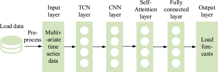
FIGURE 1. Structure of the SATCN.

3.2.1 Temporal convolutional network layer

The first layer connected to the input layer is a TCN layer, which takes the multi-dimensional time-correlated load time series, $X_{LD}=\left\{x_1,x_2,\cdot \cdot \cdot ,x_T\right\}$, as the input, and outputs the hidden states of multiple time steps utilizing TCN’s feature. This paper denotes the hidden states of multiple time steps as $H_{LD}=\left\{h_1,h_2,\cdot \cdot \cdot ,h_T\right\}$. For any time step t before the last time step T, h_t can be represented as in Eq. 18:

$h_t=F\left(x_1,x_2,\cdot \cdot \cdot ,x_t\right).(18)$

3.2.2 Convolutional neural network layer

The second layer is the CNN layer, which takes the hidden states’ output by the previous layer of TCN as the input. Leveraging the powerful feature compression and extraction capability of CNN, this layer realizes the feature recognition and extraction of the hidden states and finally outputs time series patterns $H^C$ as in Eq. 19:

$H_{i,j}^C={\displaystyle \sum }_{l=1}^T{H}_{i,l}\cdot C_{j,l},(19)$

where the subscript i represents the ith convolution layer, the subscript j represents the jth convolution kernel, and the subscript l represents the lth position in the convolution kernel. $C_{j,l}$ is the output of the jth convolution kernel at position l.

3.2.3 Self-attention mechanism layer

The third layer is the self-attention mechanism layer. First, applying the linear transformation as in Eqs 13, 14, 15, the time series features extracted by the CNN layer can be mapped to matrices Q, K, and V, and then the feature matrix Y can be calculated with a scaled dot-product attention mechanism as in Eq. 16. At last, the load forecast y_t+1 for the t+1 time step is output through a fully connected layer.

3.3 The proposed ensemble forecasting method

This paper first adopts CEEMDAN to decompose the load time series to obtain the mode components ${\overline{I}}_1,{\overline{I}}_2,...,{\overline{I}}_k$ and the residual R. Based on their permutation entropy values, they are merged to $W_1,W_2,\cdots ,W_n$, and then the CatBoost-based recursive feature reduction method is applied to extract the optimal subset of features with respect to each component W_i. Thereafter, a SATCN load forecasting model is trained to output the forecast to W_i for the next time step. The flowchart of the ensemble forecasting method is shown in Figure 2.

FIGURE 2

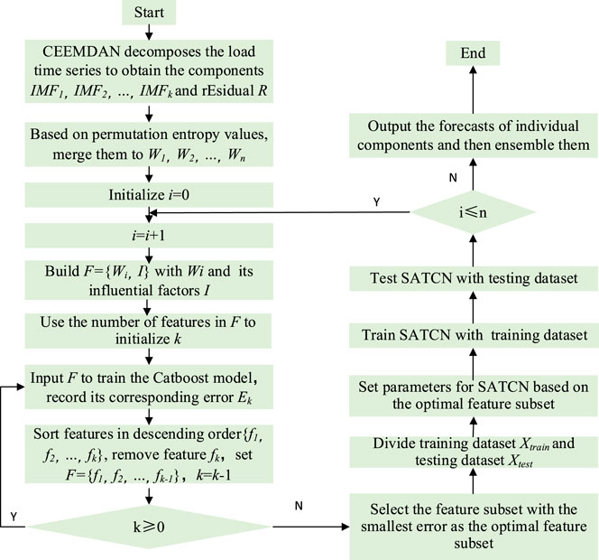
FIGURE 2. Flowchart of the ensemble forecasting method.

4 Case study

4.1 Dataset

Real electrical load data from a certain area are adopted in this paper. The dataset includes 90 days of electrical load data and related data of influencing factors from 5 July 2004 to 2 October 2004. The data granularity is hourly, i.e., 24 samples a day. Historical load, real-time temperature, time, week, month, and holiday form the input feature set as shown in Table 1. For categorical features, such as week and month, they need to be quantified into numerical values to be seamlessly input into the model. To this end, we represent hours from 0:00 to 24:00 as integers {0, 1, .., 23}, Monday to Sunday as integers {1, 2, .., 7}, and months from January to December as integers {1, 2, .., 12}. Holidays are represented as binaries {0, 1}, where 1 means that the day is a holiday; otherwise, 0. For numerical features such as load and temperature, this paper directly uses the data. Considering that the components of the load time series fluctuate periodically in days, the length of the historical load should be a multiple of one day. In this paper, 7-day historical load is selected as the input. In addition, since the time effect of temperature on the load is relatively obvious, this paper selected the temperature data of the previous 6 hours as the input.

TABLE 1

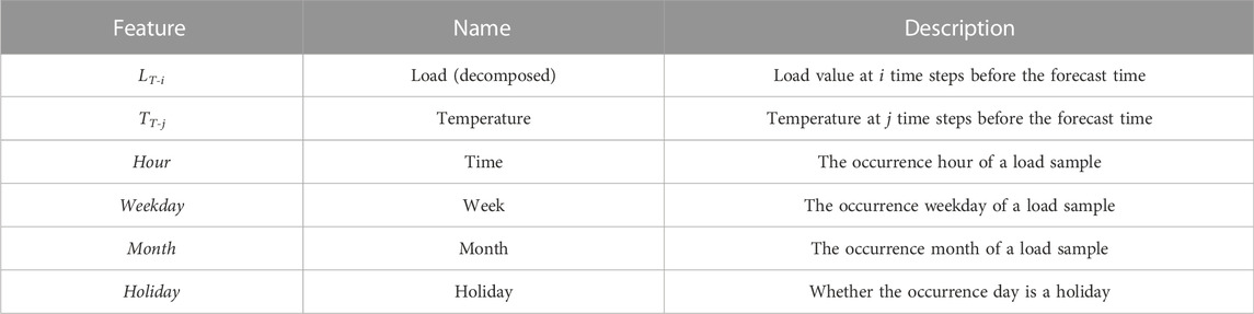
TABLE 1. Input feature set.

4.2 Performance evaluation

We use the mean absolute error (MAE), mean absolute percentage error (MAPE), and root mean square error (RMSE), as defined in Eqs 20, 21, 22, respectively, to evaluate the short-term load forecasting accuracy. In Eqs 20, 21, 22, $y_i$ and ${\widehat{y}}_i$ are the actual value and the forecast, respectively. n represents the length of the forecasts, namely, time steps.

$MAE=\frac{1}{n}{\displaystyle \sum }_{i=1}^n\left|y_i-{\widehat{y}}_i\right|,(20)$

$MAPE=\frac{1}{n}{\displaystyle \sum }_{i=1}^n\left|\frac{y_i-{\widehat{y}}_i}{y_i}\right|,(21)$

$RMSE=\sqrt{\frac{{\displaystyle \sum }_{i=1}^n\left(y_i-{\widehat{y}}_i\right.{)}^2}{n}}.(22)$

MAPE can eliminate the absolute difference between forecasting errors at different forecasting time steps by giving them the same weight, which makes MAPE highly interpretable. However, as the IMF component W_i obtained by decomposition is close to a sinusoidal curve that periodically crosses zero, when the actual value is zero or close to 0 at the forecasting time step, the MAPE will have an extremely high value causing overestimation of the forecasting error. This is because the denominator in Eq. 21 is close to 0. To this end, in the subsequent feature selection process with CatBoost, this paper uses MAE and RMSE only to evaluate the forecasting error of different feature subsets with different numbers of features.

4.3 Experimental results

4.3.1 Load time series decomposition with CEEMDAN

In the load time series decomposition with CEEMDAN, through multiple experiments, this paper sets the standard deviation of the white noise at 0.25 and generates white noise sequences 100 times. The maximum number of iterations is set to 5,000, and the results are shown in Figure 3.

FIGURE 3

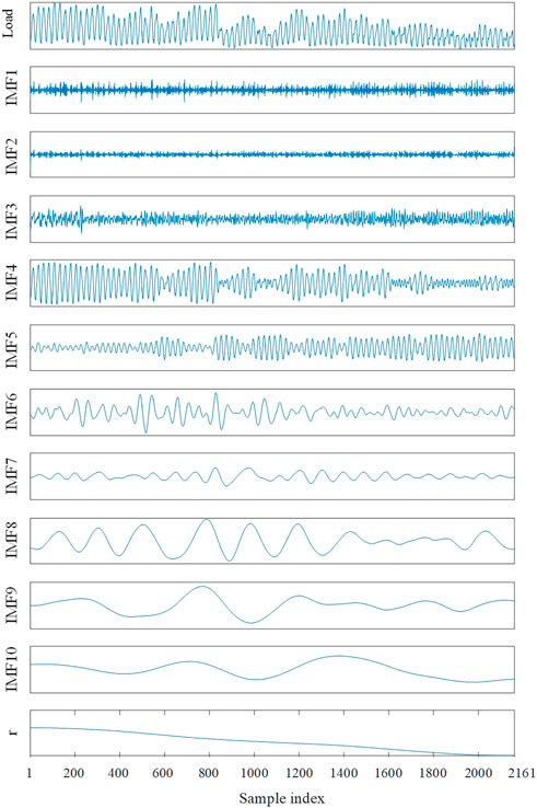
FIGURE 3. Results of CEEMDAN.

It can be seen from Figure 3 that 11 CEEMDAN IMF components are obtained by CEEMDAN. The inherent mode mixing of each IMF component is evaluated with permutation entropy, and those close IMF components are merged and reorganized. Through multiple experiments, we set τ at 1 and L at 3. The permutation entropy value of each IMF component is shown in Figure 4.

FIGURE 4

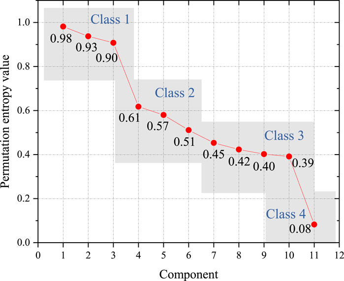
FIGURE 4. Permutation entropy values of IMF components.

From Figure 4, permutation entropy values can be clustered into three classes. The first class contains IMF components 1, 2, and 3, whose permutation entropy values are all above 0.9. Their maximum internal distance is only 0.08, while their lowest value has a distance of 0.3 to the second class. The second class contains IMFs 4–10. Their permutation entropy values are generally evenly distributed, and the descent rate gradually decreases. The third class only contains the residual component, and its permutation entropy value is only 0.08, indicating that its fluctuation pattern is extremely monotonous. This well matches the actual monotonically decreasing pattern shown in Figure 3. As the second class contains more IMF components than expected, in order to improve the overall forecasting accuracy, we further divide this class into two classes. Finally, the first divided class includes IMF components 4, 5, and 6, and the internal distance is 0.1; the second divided class includes IMF components 7, 8, 9, and 10, with an internal distance of 0.06. The final CEEMDAN IMF component merger results are shown in Table 2.

TABLE 2

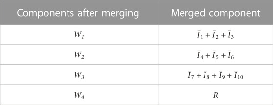
TABLE 2. CEEMDAN IMF component merger results.

Considering that the components of different fluctuation frequencies have different requirements on the model fitting ability, an appropriate network structure should be designed to avoid overfitting or underfitting and effectively improve forecasting accuracy.

4.3.2 Feature selection with CatBoost

The merged components W_i, the load combination L_T-n, temperature T_t-n, and date together constitute the original feature set F, which is input into the CatBoost gradient boosting tree. The CatBoost model is then trained. According to Eq. 10, the feature importance of individual features in F is calculated, and then these features are sorted in descending order with respect to their importance. The number of features k, the feature set F, E_MAE, and E_RMSE on the test set are recorded. Then, the feature with the lowest importance is removed from F realizing the feature reduction. This process is repeated until F becomes empty. Thereafter, the mapping between the number of input features in each component Wi and the forecasting errors, E_MAE and E_RMSE, can be established. The results are shown in Figure 5. First, the number of features corresponding to the minimum point of the E_MAE curve is selected as the optimal feature under the E_MAE index, as shown in the orange label in Figure 5; Second, the number of features corresponding to the minimum point of the E_RMSE curve is selected as the optimal feature under the E_RMSE index, as shown in the blue label in Figure 5. Finally, in order to improve the feature reduction rate and improve the forecasting efficiency, in this paper, the smaller value of E_MAE and E_RMSE is adopted to indicate the optimal feature subset.

FIGURE 5

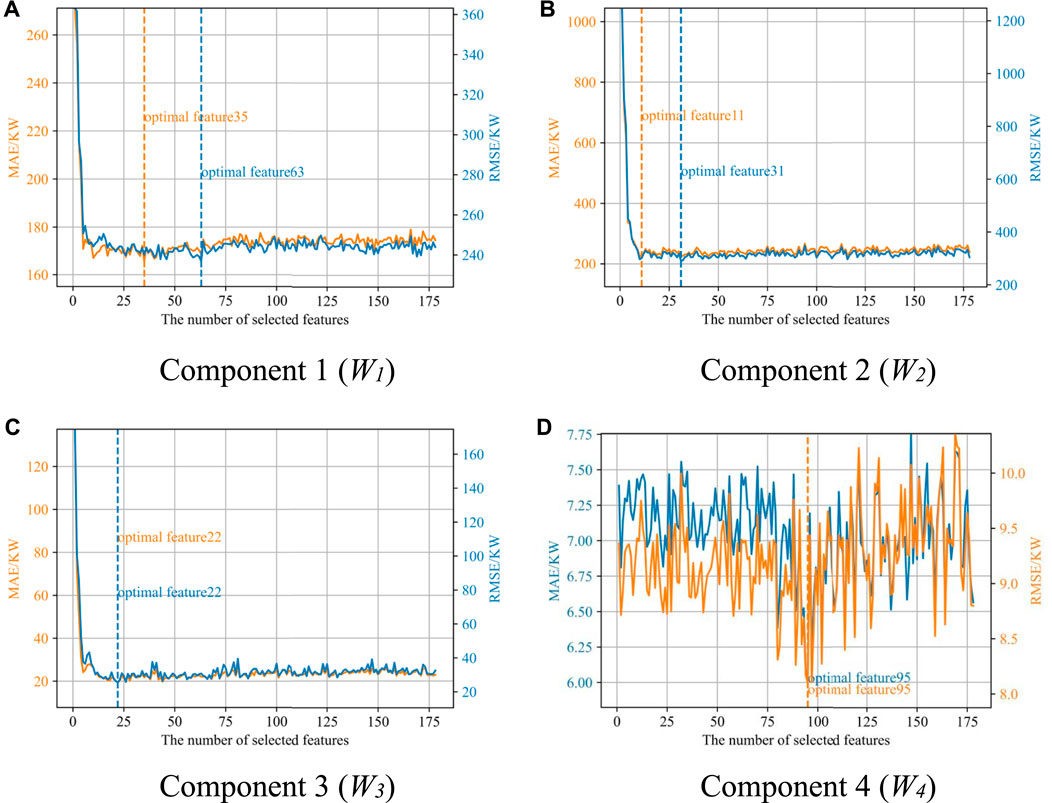
FIGURE 5. Forecasting errors with different numbers of input features for four components as examples including (A) Component 1, (B) Component 2, (C) Component 3, and (D) Component 4.

It can be seen from Figure 5 that the numbers of features in the optimal feature subsets for each component are, respectively, 35, 11, 22, and 95, and the corresponding feature reduction rates are 80.3%, 93.8%, 87.6%, and 46.6%. Generally, with the increase in the number of input features, the forecasting error first decreases greatly. Then, it gradually stabilizes and fluctuates within a small range.

The optimal value appears with a certain number of features, indicating that there are key factors affecting load forecasting accuracy. Therefore, as long as those key features are selected, relatively high forecasting accuracy can be achieved. In addition, it shows that feature selection can effectively identify the importance of different features so that redundant features and noise features can be removed to achieve dimension reduction of the input as well as training efficiency improvement. Indeed, for different components, more adaptive forecasting algorithms, models, and input structures can be designed to capture their fluctuation patterns, and the TCN with the self-attention mechanism can be applied to capture their change trends in a period of time.

4.3.3 Forecasting with the self-attention mechanism-integrated temporal convolutional network

After the optimal feature subset of each component W_i is determined, selected features will be input into the SATCN model. The optimal hyperparameters are determined with a grid search. The dataset is randomly divided into X_train, X_validation, and X_test with the ratio of 8:1:1. X_train is input into SATCN and processed sequentially by the input layer, the TCN layer, the CNN layer, the self-attention layer, and the output layer. Finally, the forecast Y_p is output. The loss function value E_loss of Y_p and label Y_T are then calculated. This paper uses Adam optimizer to realize backpropagation and update the weight W and bias b in the SATCN. This process is repeated until the E_loss of SATCN decreases slowly on X_train or E_RMSE that no longer decreases on X_validation, and this paper considers that SATCN has converged. Forecasts Y_p are obtained by inputting X_test to the trained SATCN. The summation of Y_p over components W_i gives the final forecast. The corresponding errors, E_MAPE and E_RMSE, are calculated with Eq. 20 and 21, respectively. The results are shown in Table 3.

TABLE 3

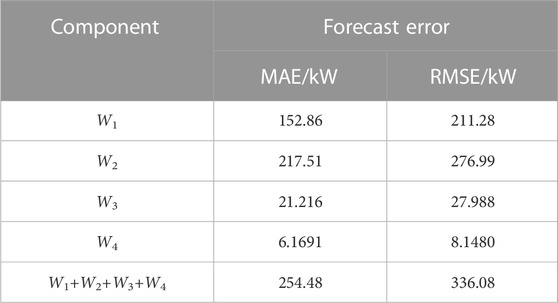
TABLE 3. Forecasting results of CEEMDAN-CatBoost-SATCN.

By setting the forecasting time steps at 24 consecutive hours of a day, the forecasting performance of individual components with the proposed CEEMDAN-CatBoost-SATCN-based method is shown in Figure 6.

FIGURE 6

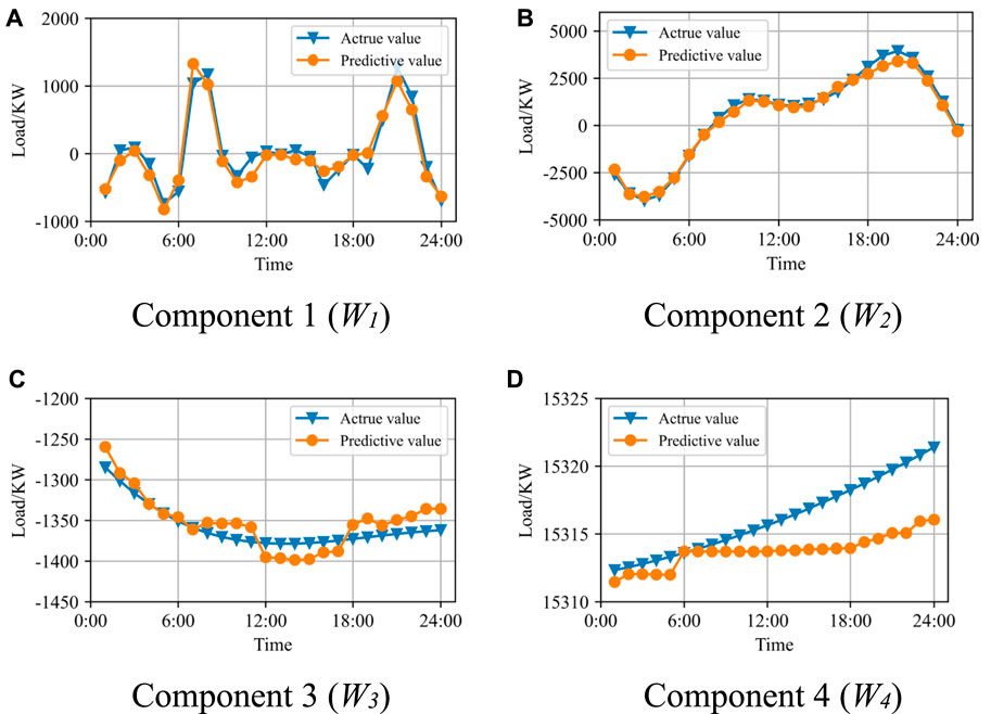
FIGURE 6. Forecasting performance of the proposed CEEMDAN-CatBoost-SATCN method with four components as examples including (A) Component 1, (B) Component 2, (C) Component 3, and (D) Component 4.

It can be seen from Table 3 and Figure 6 that for every component, E_MAE is lower than 65 KW and E_RMSE is lower than 85 KW, which indicates a high accuracy in short-term load forecasting.

4.3.4 Effectiveness of CEEMDAN and CatBoost

To verify the accuracy and efficiency of the proposed method combination of CEEMDAN-CatBoost-SATCN (denoted as method combination A), this paper compares it with SATCN (method combination B), CatBoost-SATCN (method combination C), and CEEMDAN-SATCN (method combination D). The single-time step-forecasting errors, RMSE and MAPE, are shown in Table 4, and the running time scatter diagram is shown in Figure 7.

TABLE 4

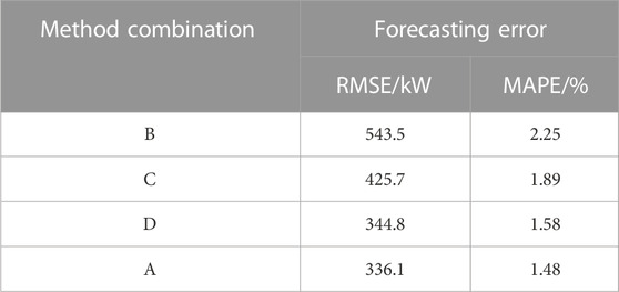
TABLE 4. Forecasting errors of different method combinations.

FIGURE 7

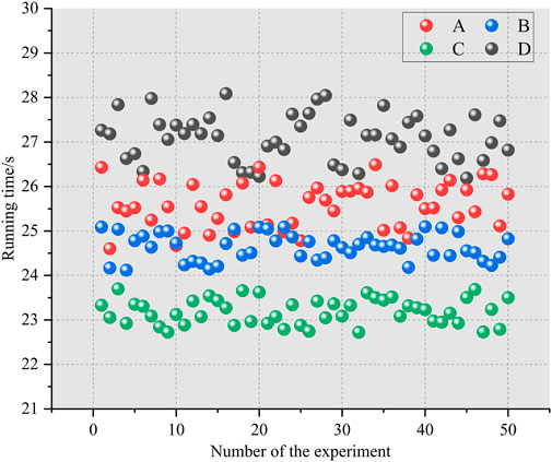
FIGURE 7. Scatter chart of running time of (A) CEEMDAN-CatBoost-SATCN, (B) SATCN, (C) CatBoost-SATCN, and (D) CEEMDAN-SATCN methods.

It can be seen from Table 4 that compared with method combination B of direct load forecasting, method combination C reduces RMSE by 21.6% and MAPE by 16%, indicating that the feature selection method can effectively improve the subsequent forecasting accuracy. CEEMDAN-based method combination D reduces RMSE by 36.5% and MAPE by 29.7%, indicating that CEEMDAN that decomposes the load time series and enables separate forecasting on components can also improve the forecasting accuracy. Compared with method combinations B, C, and D, the proposed combination, namely, method combination A, has the lowest RMSE and MAPE, which means the combination of time series decomposition and feature selection has a positive effect on improving the accuracy of short-term load forecasting.

It can be seen from Figure 7 that compared with method B, CEEMDAN has increased the complexity of model calculation and model running time due to time series decomposition, while CatBoost reduces the number of input features through feature optimization, which improves the computational efficiency. The method used in this paper combines CEEMDAN, CatBoost, and SATCN, and on the premise of significantly improving the prediction accuracy, the additional running time cost is not large.

4.3.5 Effectiveness of CEEMDAN and CatBoost

To verify the effectiveness of the proposed method in this paper, this paper compares it with BP, SVM, LSTM, GRU, and their combined methods including CEEMDAN-LSTM (CLSTM), CEEMDAN-BP (CBP), CEEMDAN-CatBoost-BP (CCBP), and CEEMDAN-CatBoost-LSTM (CCLSTM). Their performances are evaluated with MAPE and RMSE. The optimal hyperparameters of these methods are determined through multiple experiments. The single time step-forecasting errors, E_MAPE and E_RMSE, of the aforementioned models are shown in Table 5, and their forecast errors of 24-hour forecasting are shown in Figure 8.

TABLE 5

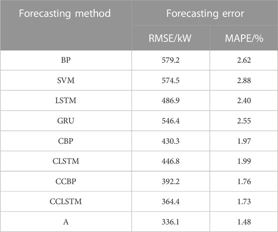
TABLE 5. Single time step forecasting error of different methods.

FIGURE 8

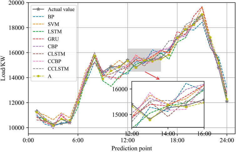
FIGURE 8. Forecasting error comparison of different forecasting methods.

It can be seen from Table 5 that CBP, which integrates the CEEMDAN based on BP, reduces E_RMSE and E_MAPE, respectively, by 25.7% and 24.8% compared with BP. CCBP that integrates CEEMDAN and CatBoost further reduces E_RMSE and E_MAPE by 8.8% and 10.6%, respectively, compared with CBP. Similarly, on the basis of LSTM, CLSTM reduces E_RMSE and E_MAPE by 8.2% and 17%, respectively; and on the basis of CLSTM, CCLSTM reduces E_RMSE and E_MAPE by 18.4% and 13.1%, respectively. This shows that CEEMDAN and CatBoost are effective in multiple forecasting models. Compared with CCBP and CCLSTM, the forecasting errors of the method proposed in this paper are smaller, which means SATCN proposed in this paper has a better forecasting performance than LSTM and BP. Moreover, compared with other forecasting methods, the method proposed in this paper has the lowest E_RMSE and E_MAPE. From Figure 8, it can be seen that in off peak load and off valley load periods, namely, from 13:00 to 15:00, the forecasting error of the proposed method is smaller compared with that in other periods.

5 Conclusion

A short-term load forecasting model considering time series decomposition and feature selection is proposed. The experimental results show that the forecasting accuracy can be effectively improved compared to traditional methods by separately selecting optimal features, building forecasting models, and finally combining the separate forecasting results with respect to the obtained components through CEEMDAN. The recursive feature selection method based on the CatBoost gradient boosting regression tree can effectively evaluate the importance of different features and remove redundant and noise features. The SATCN, integrated with the CNN and self-attention mechanism, has a strong ability to capture load time series features and explore multi-dimensional variable associations. Compared with other forecasting methods, the proposed CEEMDAN-CatBoost-SATCN-based forecasting model can accurately identify the fluctuation pattern of the load and outperform in terms of forecasting accuracy.

Data availability statement

The original contributions presented in the study are included in the article/Supplementary Material; further inquiries can be directed to the corresponding author.

Author contributions

YW, ZZ, and NP proposed the idea of the study. YW, ZZ, NP, ZS, and LX implemented the algorithms and analyzed the experimental results. All authors participated in the writing of the manuscript.

Funding

This work was supported by the funds of the Economic Research Institute of State Grid Hebei Electric Power Co. Ltd., under the Project “Optimal allocation of demand side resources based on high-dimensional spatio-temporal data under grid user two-way interaction (SGTYHT/20-JS-221).”

Conflict of interest

Authors YW, ZZ, NP, ZS, and LX were employed by the company State Grid Hebei Electric Power Co., Ltd.The authors declare that this study received funding from Economic Research Institute of State Grid Hebei Electric Power Co. Ltd.

The remaining authors declare that the research was conducted in the absence of any commercial or financial relationships that could be construed as a potential conflict of interest.

Publisher’s note

All claims expressed in this article are solely those of the authors and do not necessarily represent those of their affiliated organizations, or those of the publisher, the editors, and the reviewers. Any product that may be evaluated in this article, or claim that may be made by its manufacturer, is not guaranteed or endorsed by the publisher.

Supplementary material

The Supplementary Material for this article can be found online at: https://www.frontiersin.org/articles/10.3389/fenrg.2022.1097048/full#supplementary-material

References

AasimSingh, S. N., and Mohapatra, A. (2021). Data driven day-ahead electrical load forecasting through repeated wavelet transform assisted SVM model. Appl. Soft Comput. 111, 107730. doi:10.1016/J.ASOC.2021.107730

CrossRef Full Text | Google Scholar

Bedi, J., and Toshniwal, D. (2018). Empirical mode decomposition based deep learning for electricity demand forecasting. IEEE Access 6, 49144–49156. doi:10.1109/ACCESS.2018.2867681

CrossRef Full Text | Google Scholar

Bian, H., Wang, Q., Xu, G., and Zhao, X. (2022). Research on short-term load forecasting based on accumulated temperature effect and improved temporal convolutional network. Energy Rep. 8 (S5), 1482–1491. doi:10.1016/J.EGYR.2022.03.196

CrossRef Full Text | Google Scholar

Cao, R., Fang, L. Y., Lu, T., and He, N. J. (2021). Self-attention-based deep feature fusion for remote sensing scene classification. IEEE Geosci. Remote Sens. Lett. 18 (1), 43–47. doi:10.1109/LGRS.2020.2968550

CrossRef Full Text | Google Scholar

Chen, T., Huang, W., Wu, R., and Ouyang, H. (2021). Short term load forecasting based on SBiGRU and CEEMDAN-SBiGRU combined model. IEEE Access 9, 89311–89324. doi:10.1109/ACCESS.2020.3043043

CrossRef Full Text | Google Scholar

Deng, S., Chen, F. L., Wu, D., He, Y., Ge, H., and Ge, Y. (2022). Quantitative combination load forecasting model based on forecasting error optimization. Comput. Electr. Eng. 101, 108125. doi:10.1016/J.COMPELECENG.2022.108125

CrossRef Full Text | Google Scholar

Duygu, K. (2020). The mRMR-CNN based influential support decision system approach to classify EEG signals. Measurement 156, 107602. doi:10.1016/j.measurement.2020.107602

CrossRef Full Text | Google Scholar

Ge, L. J., Li, Y. L., Yan, J., Wang, Y. Q., and Zhang, N. (2021). Short-term load prediction of integrated energy system with wavelet neural network model based on improved particle swarm optimization and chaos optimization algorithm. J. Mod. Power Syst. Clean Energy 9 (6), 1490–1499. doi:10.35833/MPCE.2020.000647

CrossRef Full Text | Google Scholar

Hancock, J. T., and Khoshgoftaar, T. M. (2020). CatBoost for big data: An interdisciplinary review. J. Big Data 7 (1), 94. doi:10.1186/s40537-020-00369-8

PubMed Abstract | CrossRef Full Text | Google Scholar

Hu, J. M., Luo, Q. X., Tang, J. W., Heng, J. N., and Deng, Y. W. (2022). Conformalized temporal convolutional quantile regression networks for wind power interval forecasting. Energy 248, 123497. doi:10.1016/J.ENERGY.2022.123497

CrossRef Full Text | Google Scholar

Huang, L., Chen, S. J., Ling, Z. X., Cui, Y. B., and Wang, Q. (2021). Non-invasive load identification based on LSTM-BP neural network. Energy Rep. 7 (S1), 485–492. doi:10.1016/j.egyr.2021.01.040

CrossRef Full Text | Google Scholar

Jiang, H. W., Zou, B., Xu, C., Xu, J., and Tang, Y. Y. (2020). SVM-Boosting based on Markov resampling: Theory and algorithm. Neural Netw. 131, 276–290. doi:10.1016/j.neunet.2020.07.036

PubMed Abstract | CrossRef Full Text | Google Scholar

Li, C., Li, G., Wang, K., and Han, B. (2022). A multi-energy load forecasting method based on parallel architecture CNN-GRU and transfer learning for data deficient integrated energy systems. Energy 259 (15), 124967. doi:10.1016/J.ENERGY.2022.124967

CrossRef Full Text | Google Scholar

Li, S. Q., Xu, Q., Liu, J. L., Shen, L. Y., and Chen, J. D. (2022). Experience learning from low-carbon pilot provinces in China: Pathways towards carbon neutrality. Energy Strategy Rev. 42, 100888. doi:10.1016/J.ESR.2022.100888

CrossRef Full Text | Google Scholar

Luo, H. F., Dou, X., Sun, R., and Wu, S. J. (2021). A multi-step prediction method for wind power based on improved TCN to correct cumulative error. Front. Energy Res. 9. doi:10.3389/FENRG.2021.723319

CrossRef Full Text | Google Scholar

Ma, X. J., Sha, J. L., Wang, D. H., Yu, Y. B., Yang, Q., and Niu, X. Q. (2018). Study on a prediction of P2P network loan default based on the machine learning LightGBM and XGboost algorithms according to different high dimensional data cleaning. Electron. Commer. Res. Appl. 31, 24–39. doi:10.1016/j.elerap.2018.08.002

CrossRef Full Text | Google Scholar

Mangalathu, S., Jang, H., Hwang, S. H., and Jeon, J. S. (2020). Data-driven machine-learning-based seismic failure mode identification of reinforced concrete shear walls. Eng. Struct. 208, 110331. doi:10.1016/j.engstruct.2020.110331

CrossRef Full Text | Google Scholar

Rehman, A. U., Wadud, Z., Elavarasan, R. M., Hafeez, G., Khan, I., Shafiq, Z., et al. (2021). An optimal power usage scheduling in Smart grid integrated with renewable energy sources for energy management. IEEE ACCESS 9, 84619–84638. doi:10.1109/ACCESS.2021.3087321

CrossRef Full Text | Google Scholar

Tan, M., Yuan, S., Li, S., Su, Y., Li, H., and He, F. (2020). Ultra-short-term industrial power demand forecasting using LSTM based hybrid ensemble learning. IEEE Trans. Power Syst. 35 (4), 2937–2948. doi:10.1109/TPWRS.2019.2963109

CrossRef Full Text | Google Scholar

Xiao, L., Li, M., and Zhang, S. (2022). Short-term power load interval forecasting based on nonparametric bootstrap errors sampling. SSRN J. 8, 6672–6686. Social Science Electronic Publishing. doi:10.2139/ssrn.3927002

CrossRef Full Text | Google Scholar

Ye, Y., Wang, L., Wang, Y., and Qin, L. (2022). An EMD-LSTM-SVR model for the short-term roll and sway predictions of semi-submersible. Ocean. Eng. 256 (15), 111460. doi:10.1016/J.OCEANENG.2022.111460

CrossRef Full Text | Google Scholar

Yuan, F., and Che, J. (2022). An ensemble multi-step M-RMLSSVR model based on VMD and two-group strategy for day-ahead short-term load forecasting. Knowledge-Based Syst. 252, 109440. doi:10.1016/J.KNOSYS.2022.109440

CrossRef Full Text | Google Scholar

Zhang, W. G., Wu, C. Z., Zhong, H. Y., Li, Y. Q., and Wang, L. (2020). Prediction of undrained shear strength using extreme gradient boosting and random forest based on Bayesian optimization. Geosci. Front. 12 (1), 469–477. doi:10.1016/j.gsf.2020.03.007

CrossRef Full Text | Google Scholar

Zhang, W. Y., Qu, Z. X., Zhang, K. Q., Mao, W. Q., Ma, Y. N., and Fan, X. (2017). A combined model based on CEEMDAN and modified flower pollination algorithm for wind speed forecasting. Energy Convers. Manag. 136, 439–451. doi:10.1016/j.enconman.2017.01.022

CrossRef Full Text | Google Scholar

Zhao, C., Sun, J., Lin, S., and Peng, Y. (2022). Rolling mill bearings fault diagnosis based on improved multivariate variational mode decomposition and multivariate composite multiscale weighted permutation entropy. Measurement 195, 111190. doi:10.1016/J.MEASUREMENT.2022.111190

CrossRef Full Text | Google Scholar

Zhou, Y. R., Li, T. Y., Shi, J. Y., and Qian, Z. J. (2019). A CEEMDAN and XGBOOST-based approach to forecast crude oil prices. Complexity 2019, 1–15. doi:10.1155/2019/4392785

CrossRef Full Text | Google Scholar

Zhu, R. J., Liao, W. L., and Wang, Y. S. (2020). Short-term prediction for wind power based on temporal convolutional network. Energy Rep. 6 (9), 424–429. doi:10.1016/J.EGYR.2020.11.219

CrossRef Full Text | Google Scholar