Circulation patterns identified by spatial rainfall and ocean wave fields in Southern Africa

1. Introduction

Local weather (precipitation, temperature wind) and related phenomena such as floods, storm, and waves are strongly dependent on atmospheric processes. These processes are very complex and highly non-linear. On the other hand due to the continuity of the atmospheric conditions these local phenomena are imbedded into large scale features. It is both of theoretical and practical importance to understand these links. Among the atmospheric variables, pressure is the driver for flow and transport. Air pressure at the land surface is a variable which can be measured simply and with good accuracy. Selected observations and meteorological models provide information on high altitude pressure conditions. Air pressure and geopotential heights are among the best modeled quantities. Therefore, it is reasonable to use them as a basis to describe atmospheric circulation.

The relationship between local variables and atmospheric circulation described with the help of pressure conditions is a complicated and highly non-linear one. On the other hand it reasonable to assume that similar circulation conditions cause similar local meteorological conditions. Therefore, an appropriate classification can help to quantify the relationship between local variables, such as amount of rain on a day in a region or wave height and period on a shoreline, and circulation. The intention is to define classes on the basis of the circulation and the local variables via conditional distributions. The behavior of the local variable described for example using the conditional distribution should be different for the different classes from the unconditional distribution of the variable. A comprehensive summary of classification methods can be found in Jacobeit (2010).

There are different ways one can define groups of circulation patterns (CPs):

1. to define CPs using atmospheric variables only

2. to define CPs using atmospheric variables by taking the local variable into account for setting up the patterns

3. to define CPs using a combination of atmospheric variables and local variables

The first method intends to find typical distinct patterns of the atmospheric variables. The patterns differ in their defining space. Their link to local variables is determined after the classification and might for some variables yield a good distinction in the behavior while for others not.

The second method acknowledges the fact that relatively small differences of the atmospheric variables might lead to very different behavior of the local variables. This means that the classification should not intend to distinguish the patterns by producing very different CPs but to group CPs which to some extent are similar but explain the target variable as well as possible. On the other hand it is important that the classification is done on the basis of the atmospheric variables only so that the classification can be used for time periods lacking the observation of the local variables.

The goals of various classification schemes can differ widely. While the classification of pressure fields on a purely statistical basis might reveal specific features of atmospheric dynamics, it might not provide the best basis for the explanation of the behavior of surface variables such as wind, temperature or precipitation. Under certain circumstances relatively small differences in the atmospheric conditions can lead to very different behavior of the surface variables. If one is interested in explaining the relationship between surface variables and atmospheric conditions then the purpose is to obtain classes of CPs with distinct conditional probabilities or distributions of the selected variables.

The first classifications were developed for regions in Europe on a subjective basis (Lamb, 1972 for Great Britain and Hess and Brezowsky, 1952 for Germany). Automated classifications were developed for different regions in Europe, North America, and China. In this paper fuzzy rule based classifications are developed for precipitation and waves in South Africa.

2. Methodology

The basic methodology of fuzzy rule-based classification was described for explaining precipitation behavior in Bárdossy et al. (1995). The main ideas are summarized here.

The classification is performed on anomalies of daily air pressure based variables: sea level pressures or geopotential heights g. These data can be obtained from reanalysis products on a regular grid. The anomalies are calculated under consideration of the annual cycle of both the mean and the standard deviation of the observed pressure. The anomaly at gridpoint x and time t is calculated as:

$\begin{array}{cc}d(x,t)=\frac{g(x,t)-\overline{g}(x,\text{J}(t))}{s_g(x,\text{J}(t))}& \left(1\right)\end{array}$

where J(t) is the Julian date corresponding to day t (which is a value between 1 and 366), g(x, J(t)) is the mean and s_g(x, J(t)) is the standard deviation of g at location x and Julian day J(t). These anomalies d have zero mean and unit standard deviation for each grid location.

The classification is based on the location of certain anomalies. For each gridpoint x of the pressure grid G five different possibilities of anomalies are considered to define a classification class. A triangular fuzzy number is assigned to each of these possible anomalies:

1. positive anomaly (0, 3, +∞)_T

2. negative anomaly (− ∞, −3, 0)_T

3. non-positive anomaly (−4, −0.85, 0.25)_T

4. non-negative anomaly (0.25, 0.85, 4)_T

5. non-representative anomaly (− ∞, 0, +∞)_T

where the subscript T denotes a triangular fuzzy number with the membership function:

$\begin{array}{cc}{\mu }_{{(a,b,c)}_T}(d)=\{\begin{array}{ll}\frac{d-a}{b-a}\hfill & \text{ if }a\le d\le b\hfill \\ \frac{d-c}{b-c}\hfill & \text{ if }b<d\le c\hfill \\ 0\hfill & \text{ else}\hfill \end{array}& \left(2\right)\end{array}$

This means that for the classification of each gridpoint one of the above possible classes is assigned. Thus, a class k can be defined as a vector j_k(x)x ϵ G where each j_k(x) is an integer such that 1 ≤ j_k(x) ≤ 5.

For a given day t and a given set of rules j_k(x) x ϵ G and k = 1, …, K the classification is performed as follows:

1. For each rule k and each location x the membership value of d(x, t) in the fuzzy set corresponding to j_k(x) is calculated. These values are μ_jk(x) (d(x, t))

2. These individual membership values are combined to an overall degree of fulfillment of the rule k by calculating:

$\begin{array}{cc}\text{DOF}(k,t)={\displaystyle \prod _{m=1}^4{\left[\frac{1}{\#\{x{j}_k(x)=m\}}{\displaystyle \sum _{x|j_k(x)=m}{\mu }_{j_k(x)}}{(d(x,t))}^{q_m}\right]}^{\frac{1}{q_m}}}& \left(3\right)\end{array}$

3. The k₀ index corresponding to the maximal DOF(k, t) is selected as class for day t

For further details the readers are referred to Bárdossy et al. (1995).

The fuzzy rule based classification is performed to explain the behavior of one or more selected variables. These are denoted with the variable V. Two types of objective functions are considered. The first one relates the CPs to the exceedance of certain thresholds of V. The objective is to define classes with frequencies of exceedances which differ from the unconditional frequency of occurrences. The first is O₁:

$\begin{array}{cc}{O}_1(\theta )={\left({\displaystyle \sum _{t=1}^T{\left(h_{CP(t)}(V>\theta |CP(t))-h(V>\theta )\right)}^2}\right)}^{\frac{1}{2}}& \left(4\right)\end{array}$

where h stands for the frequency of an event, V is the variable under interest and θ is a prescribed threshold. This objective expresses that a classification should help to decide if a threshold is exceeded or not.

The second objective type is related to the mean magnitude of the variable V with respect to the CPs. It is formulated as:

The second objective function evaluates the ability of the algorithm to derive classes with average values of V that are different from the unclassified average. In other words this objective function measures the separability of the classes from the mean.

These objective functions can be used in combination—for example for different thresholds θ and even for different variables. A weighted combination of them is used as the classification objective function.

The value of the objective functions depends on the classification, which itself depends on the selected rules {j_k(x)x ϵ G k = 1, …, K}, where K is the number of rules. Once objective functions for the classification are defined, different classifications can be compared with respect to their ability to explain the variability of the surface variable investigated. The higher the objective function values the better the classification is. Thus, one can use an optimization procedure to find rules j_k(x) which maximize the objective functions. The number of possible rule systems for a given number of patterns is given by the combinatorial:

$N_K=\left(\begin{array}{c}{5}^{\left|G\right|}\\ K\end{array}\right)$

This is usually an extremely large number (for example for a small pressure grid 10 × 10 with |G| = 100 nodes and K = 10 rules the number of possible rule systems is > 10³⁴⁰) thus the best rules cannot be found by trying all possibilities. Instead an optimization method has to be applied. Simulated annealing provides a reasonable alternative as described in Bárdossy et al. (2002).

2.1. Classification Quality

The quality of the classification can be measured by the above defined objective functions. Besides that other measures can be defined, which can be used for comparison, for example to find the optimal number of classes. For this one can use thresholds for the variable V. The entropy of the conditional distributions can be used to measure the binary quality of a classification:

$\begin{array}{cc}H(K)={\displaystyle \sum _{k=1}^K{h}_k}\left(p_k{\log }_2{p}_k+(1-p_k){\log }_2(1-p_k)\right)& \left(6\right)\end{array}$

where p_k is the probability of the exceedance of the threshold on a day with the k-th CP, and h_k is the frequency of the k-th CP. The quantity H(0) is the entropy in the case no classification was performed:

$\begin{array}{cc}H(0)=p_0{\log }_2{p}_0+(1-p_0){\log }_2(1-p_0)& \left(7\right)\end{array}$

A classification provides information for the variable V if H(K) < H(0). In general a classification using K classes is better than another with L classes if:

$H(K)<H(L)$

2.2. Non-Uniqueness Issues

Different CP classifications can be obtained for the same region. In Philipp et al. (2014) the authors investigated 27 automatic CP classification approaches and found that different classification methods lead to very different classifications. The Fuzzy Rule Based classification method can lead to different classifications as the stochastic optimization obtained using simulated annealing does not necessarily lead to the same classification if another sequence of random numbers is selected. A different choice of stations or a different choice of thresholds or weights for the objective functions can lead to different classifications too. Different classifications can be compared from the viewpoint of their performance or from the viewpoint of the similarity of their classes. While the calculation of the objective functions is straightforward, the similarity of the classifications requires further measures.

Two statistics can be calculated based on the contingency tables of the pairs of classifications. For two different classifications n_ij is the number of days in class i for the first and in class j in the second classification. The χ² statistics to compare the classifications is calculated as:

$\begin{array}{cc}{\chi }^2={\displaystyle \sum _{i=1}^r{\displaystyle \sum _{j=1}^s\frac{{\left(n_{ij}n-n_{i·}{n}_{·j}\right)}^2}{n_{i·}{n}_{·j}n}}}& \left(8\right)\end{array}$

where r is the number of classes in the first classification, s is the number of classes in the second classification, n_i· is the number of days in class i for the first classification, n_·j is the number of days in class j for the second classification and n is the total number of days. If the classifications are independent then the χ² value is small, the bigger it is the more the classifications resemble each other. Based on the χ² values two measures of dependence were calculated, the modified Pearson coefficient C:

$\begin{array}{cc}C=\sqrt{\frac{\min (r,s)}{\min (r,s)-1}}\sqrt{\frac{{\chi }^2}{{\chi }^2+n}}& \left(9\right)\end{array}$

and the Cramer coefficient (Hartung et al., 2005) V:

$\begin{array}{cc}V=\sqrt{\frac{{\chi }^2}{n(\min (r,s)-1)}}& \left(10\right)\end{array}$

Both coefficients are bounded by 1, and the higher they are the stronger the association is. The associations of CP classifications for the same geographical regions using different objective functions or different stochastic optimization settings are usually strong, which is a consequence of the fact that the same variables (geopotential heights) are classified.

2.3. Data Used

The classifications were performed using ECMWF ERA reanalysis data sets. The classification is based on daily normalized anomalies, derived from the 700 hPa geopotential height with a grid resolution of 2.5^o (10^o—50^o S; 0^o—50^o W). Geopotential heights were obtained from the ERA-Interim data set of Dee et al. (2011) for the period 1979–2009 (http://apps.ecmwf.int/datasets/).

3. Classification for Precipitation

3.1. Objective Functions

Precipitation has a highly skewed distribution with above 80% probability of a dry day in many parts of South Africa. Individual very high values of precipitation can lead to “random” optima which are not robust. Instead a new variable related to the average wetness of a selected number of stations was considered:

$\begin{array}{cc}W(t)=\frac{\#\{x_i;Z(x_i,t)>0\}}{\#\{x_i;Z(x_i,t)\ge 0\}}& \left(11\right)\end{array}$

by definition 0 ≤ W(t) ≤ 1. This variable is taken as V for the objective functions in Equations (4, 5).

The 24 Climate Regions defined by Kruger (2004), slightly modified by concatenating some of the very small regions (mostly in dry areas) with larger ones, were used for the classification. The map with the locations of the regions is shown in Figure 1. A set of representative stations was selected for each region and the CPs were classified using the above defined objective function. The classification obtained using this objective function works well for precipitation in all selected regions both for the calibration and the validation time periods. For variety, we will show some CPs and resulting rainfall in Figure 2 and specific CPs selected for region 6 in Figure 3.

FIGURE 1

Figure 1. The Kruger climate regions of South Africa after (Kruger, 2004).

FIGURE 2

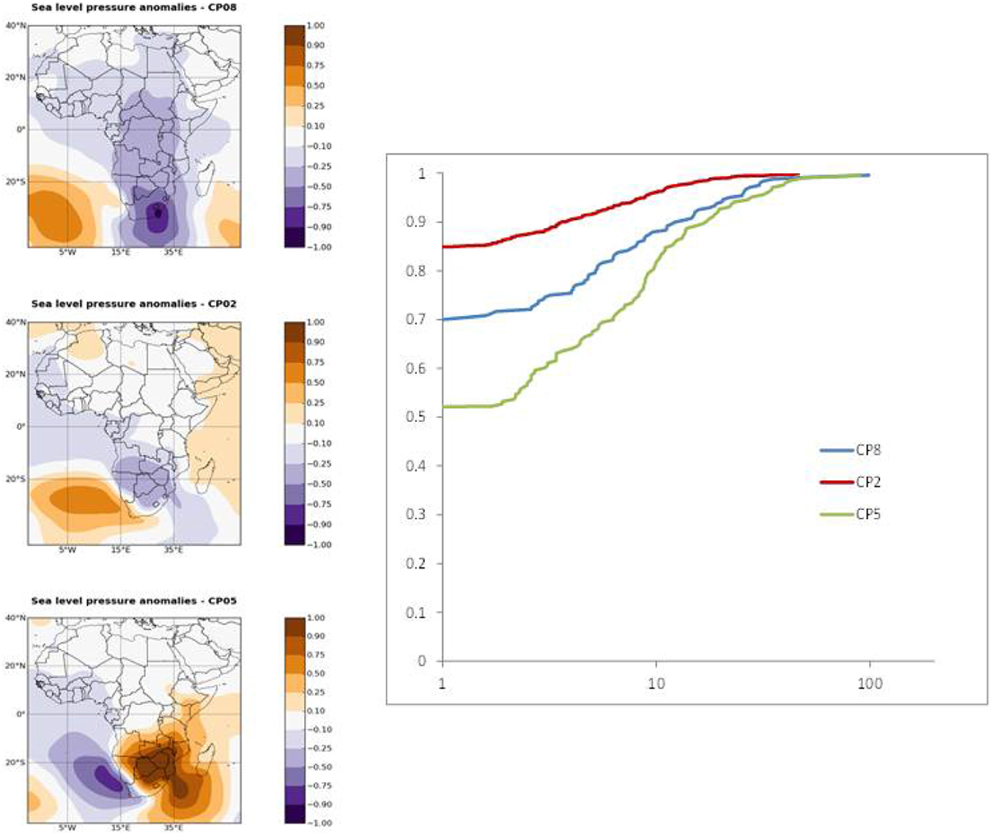
Figure 2. Three different CPs and the related distributions of daily precipitation in Mpumalanga in Region 5 of Figure 1. The maps on the left are CPs 8, 2, and 5, appearing as blue (middle), red (dry), and green (wet) lines in the figure of frequency distributions.

FIGURE 3

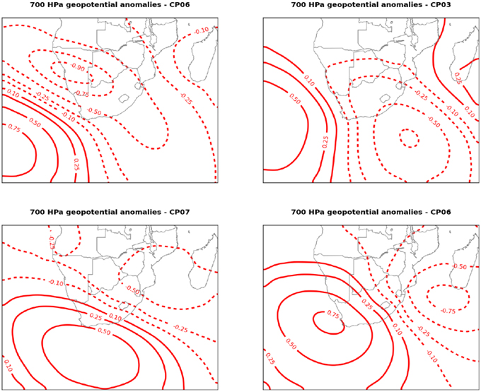
Figure 3. Two pairs of CPs: top two similar to each other and the bottom two likewise, selected from the CPs chosen on 2 sets of gauges in Region 6.

3.2. Spatial Extent of Classification and Non-Uniqueness of CP Set Selection

We explore three sets of classifications driven by precipitation wetness. The first CP set is conditioned on wetness in region 5 and we compare the differences in rainfall distributions from three distinct sets of CPs. The second set involves determining the robustness of the method when different sets of gauges in a region are used for CP classification. For this purpose we use data from region 6 and randomly sample 2 sets for comparison. The third experiment treats CPs defined over three regions in Figure 1. These are region 6 which experiences subtropical summer rainfall and the occasional hurricane, 10 which is typically savannah, experiencing summer rainfall dominated by convective systems, and 22 which has a Mediterranean climate and experiences mostly frontal system winter rainfall.

Due to the stochastic optimization no unique best classification can be achieved. It is of interest to see how

• the selection of the stations for the objective function

• the randomness due to stochastic optimizations

influences the results. For this purpose the performance measures were calculated for different classification results.

To introduce the first experiment, which is to demonstrate the link between rainfall regimes and CPs, we offer Figure 2, which shows the correspondence between (i) three CPs chosen from a set of 8 in Mpumalanga and (ii) the rainfall distribution at a particular rain-gauge in the region. Figure 2 shows the 700 hPa anomalies for three selected CPs and the corresponding distributions of daily precipitation. CP2 is the driest with the highest probability of a dry day. CP5 is the wettest with a much lower probability of a dry day. CP8 is medium wet with statistics between CP5 and CP2. The distributions are significantly different from each other indicating that classification provides useful information on precipitation behavior.

To illustrate the methodology applied in the second experiment, we selected region 6, then we selected some gauges within the region, in different configurations, to classify the Circulation Pattern anomalies [CPs] which are the cause of different types of rainfall over this region.

We find we get similar CPs, enough similarity of shape to pick a set, [note that the labeling within each set is random, so we match by correlation of shape, not label]. Figure 3 shows the 700 hPa anomalies for two different classifications.

This similarity allows us to settle on one set of CPs per region (and season) because we have a robust method. In the next section we turn to the Infilling/repair problem an extension of which we will use later in spatial interpolation between gauges.

The third experiment was to make comparisons between CP sets within and between 3 regions. This started by selecting 5 random subsets of 12 gauges from the historical datasets in each of the regions. CPs were conditioned on each of the 5 subsets in each region independently. We then set out to determine whether the similarity of the sets within each region was materially greater than between regions. Because these are categorical data it does not make sense to compute correlation coefficients between sets, so Pearson and Cramer coefficients (Equations 9, 10) based on the χ² were the statistics used.

We chose three climate regions within South Africa to compare sets of CPs. The regions chosen and shown in Figure 1 are: region 6 (KwaZulu-Natal), region 10 (Free State), and region 22 (Western Cape). We used 5 different random groupings of gauges for classifications in each region, thus for each region we derived 5 independent sets of CPs, making 15 in all.

The purpose of this calculation was to determine if the CPs derived for a given region had a higher inter-association than between regions. These coefficients were calculated for all pairs of classifications for the same regions. Then the averages of the association measures were calculated for classifications corresponding to the same (excluding the comparison of a classification with itself), and corresponding to different regions leading to 2 sets of 3 by 3 matrices.

The average of the 20 within-region statistics are compared with the averages of the 25 between-region statistics and appear in Tables 1, 2 (the difference in the numbers in each group is because we omitted the diagonal elements of comparing a set with itself). The result is that there is a significant difference between the within against the between coefficients, supporting our exploitation of this CP selection procedure based on daily wetness.

TABLE 1

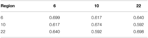
Table 1. CP similarities for different classifications using the Pearson coefficient in the regions numbered 6, 10, and 22 in Figure 1.

TABLE 2

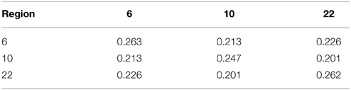
Table 2. CP similarities for different classifications using the Cramer coefficient in the regions numbered 6, 10, and 22 in Figure 1.

All classifications show significant dependence, which of course is reasonable as the atmospheric conditions on the same region are classified in all cases. On the other hand the within block average statistics are larger than the between block counterpart, inferring that there is a stronger within relationship than between blocks. The conclusion is that the choosing of CPs dependent on regions is valuable and worth the effort.

4. Classification for Waves

Atmospheric circulations drive regional wave climates through atmosphere-ocean interactions. In particular they control the generation of the extreme wave events that cause severe coastal erosion. They are therefore also fundamental drivers of coastal vulnerability. The link between the wave climates and atmospheric circulation is complex. However, statistical models that link synoptic scale atmospheric circulation to regional wave characteristics have recently been shown to give significant insights (Pringle et al., 2014). We propose that the classification of atmospheric drivers can improve coastal vulnerability assessments and the prediction of climate change effects. For example it provides a natural way to identify and isolate the effects of independent storm events, which is required for extremum analysis. For example (Corbella and Stretch, 2012a) identified independent events based on the autocorrelation or by using a 6-h inter-arrival window. The transition of CPs between classes is a physically more meaningful method for defining independent events. Atmospheric CPs also contain important information regarding the distribution of wave height, direction and period, because when a particular CP type occurs the associated wave height, direction, and period can be (statistically) predicted. Linking wave events to CPs can also be used to extend current data sets and to infill missing data (Hewitson and Crane, 2002). Finally the prediction and evaluation of climate change impacts on coastal vulnerability would be more robust if linked to changes in the atmospheric CPs that are the basic drivers of wave climates and extreme wave events.

4.1. Case Study Description

The KwaZulu-Natal (KZN) coastline (Figure 4) is associated with a high energy wave climate. A number of weather types have been cited as the drivers of this wave climate. For example tropical cyclones, mid-latitude (extra-tropical) cyclones and cut off lows (Rossouw et al., 1982; Corbella and Stretch, 2012c; Mather and Stretch, 2012). The location and persistence of tropical cyclones (TC's) are believed to drive large wave events that cause severe beach erosion in KZN (Corbella and Stretch, 2012c; Mather and Stretch, 2012). Cut-off lows are deep low pressure systems that are displaced from the normal path of west-east moving mid-latitude cyclones (Preston-Whyte and Tyson, 1988). They are caused by instabilities within the westerly zonal flow due to the high wind shear. Vortices can become cut-off and move equator-ward (Preston-Whyte and Tyson, 1988). These features lead to seasonality in the wave climate and the occurrence of storms in particular. On average autumn and winter (April to September) are associated with the largest wave energy, while summer (January to March) has the smallest (Corbella and Stretch, 2012c). The significant wave height (Hs) is the key variable of interest for coastal vulnerability applications. Our algorithm considers both the daily average significant wave height and the daily maximum significant wave height. Wave data for the period 1992–2009 were obtained from wave buoys located near Durban and Richards Bay on the KZN coastline (Figure 4).

FIGURE 4

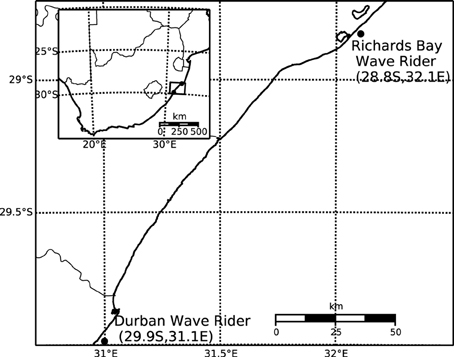
Figure 4. Locations of the wave observation buoys at Durban and Richards Bay, along the KwaZulu Natal coastline.

In this application the goal of the classification is to obtain a set of CP classes which explain extreme wave events. Wave heights larger than 3.5 m have been shown to cause significant erosion along the KZN coastline (Corbella and Stretch, 2013). The objective functions (Equations 4, 5) were used as performance measures.

The wave height threshold θ can be exploited to incorporate various scenarios. Two different thresholds were used. The first relates to the occurrence of extreme events (θ₁ = 3.5 m), while the second relates to midrange wave heights (θ₂ = 2.5 m). The second objective function type is also used to provide a more detailed classification.

To account for the persistence of CPs during extreme events (Equation 4) was modified to include storm durations, defined as the duration of wave height excursions above 3.5 m.

4.2. Dominant CP Classes

Figure 5 shows the average anomaly patterns for all the CP classes. CP99 refers to an unclassified class. Useful statistical parameters for each CP class are their frequency of occurrence, their contribution to extreme events, and the average and maximum significant wave heights (H_s) associated with them. These parameters are shown in Table 3.

FIGURE 5

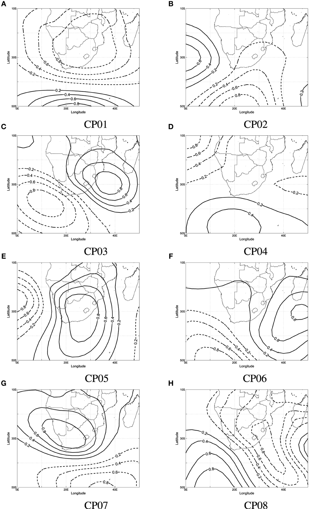
Figure 5. Average anomaly patterns for 8 CP classes derived from the regional wave climate data. Negative (low) pressure anomaly contours are shown as solid lines while positive pressure contours are dashed.

TABLE 3

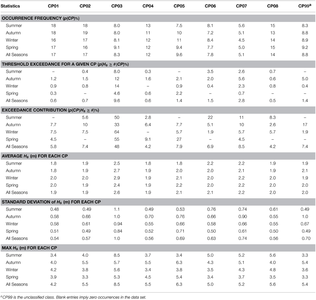
Table 3. CP Occurrence frequencies and wave height statistics associated with each CP class.

The results reflect a number of trends in CP-wave generation. However, only the two most significant trends are discussed herein. Firstly CP01 and CP02 (Figure 5A) occur most frequently (about 17% of the time). Both CP classes resemble a mid-latitude cyclone in its different stages of development. The CP01 resembles the central low pressure region of a mid-latitude cyclone as it moves from west to east south of the country, while CP02 resembles the high-pressure region that follows. Secondly, Table 4 shows a class (CP03) that comprises 60% of all extreme wave events. The CP03 is shown to contribute significantly to extreme events all year round with highest contribution in winter (65%). However, CP03 (Figure 5C) occurs infrequently (9% of the time). Its occurrence is associated with large average and maximum significant wave heights ranging from 2.4 to 3.0 m and 5.0 to 8.5 m, respectively. CP05 and CP06 (Figures 5E,F) contribute approximately to 30% of extreme events in spring and summer, respectively. The CP06 resembles a pattern similar to TC's south of Madagascar. TC's located within this region have been cited to drive large swells toward the KZN Coast (Mather and Stretch, 2012). The CP05 resembles low-pressure systems over the interior.

TABLE 4

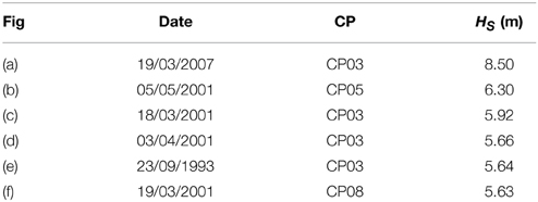
Table 4. Six of the most extreme wave events on record and their associated CPs for the period 1992–2009.

The algorithm only considered CPs associated with extreme events at the time the event was recorded. In other words no time lags were considered when deriving the CP classes. Therefore, the algorithm assumes that extreme events are driven by relatively stationary CPs.

4.3 CP Variability

The degree of fit (DOF) describes the membership of a CP for given day to a particular class. The larger the DOF the stronger the belief that the CP belongs to a particular class. Figure 6 shows the average anomaly pattern for CP03 and the CPs associated with both the strongest and weakest membership for that class. CP03 is associated with a strong low pressure region east/south-east of South Africa. The pattern also shows a strong high-pressure region to the southwest. The coupling between the strong low and high pressure drive strong winds and subsequently large waves toward the coastline. The CP with the weakest membership to CP03 is shown to be a weak anomaly pattern (refer to Figure 6C).

FIGURE 6

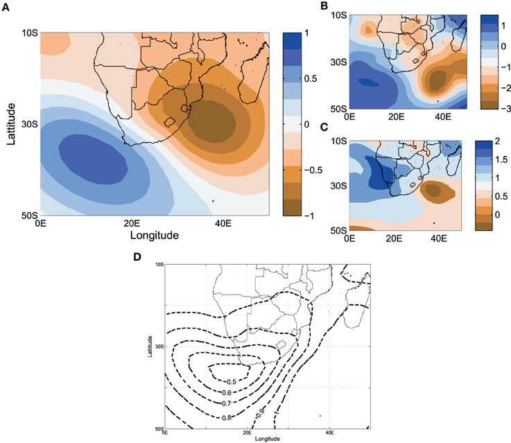
Figure 6. Average anomaly pattern for CP03 (A) showing (B) the anomaly with highest DOF, (C) the anomaly with lowest DOF value, and (D) the standard deviation for all CP03 anomalies.

4.4. Variability within Classes

It is expected that in regions of high pressure pattern variation should be low. This is attributed to the stability of high pressures in their positions. In contrast pattern variation in regions of low pressure should be higher primarily due to the movement of low pressure systems. This is reflected in Figure 6D, which shows significantly larger variation (standard deviation of 1) in the vicinity of the low-pressure region. The magnitude of the variation also indicates that CPs driving extreme events are associated with strong low pressures.

4.5. CP Rules and Extreme Events

Daily CP realizations associated with extreme wave events (H_s ≥ 3.5 m) were compared to the average class pattern to which they belong. Figure 7 shows the average pattern for CP03 together with selected extreme events corresponding to CP03. The locations of the peak negative anomalies are shown in the plot. Significant pattern variability within the class is apparent. Figure 8 and Table 4 show the CPs associated with six of the largest significant wave height events. The majority of the six events have been classified as belonging to CP03. Figure 8F from visual inspection shows a pattern similar to CP04 and CP08. Both classes are associated with low-pressure regions southeast of Madagascar. However, the CP has been classified as belonging to class CP08 and not CP04. From a visual account it appears to better resemble class CP04. Figures 8A,C are the CPs associated with the March 2007 storm which caused severe coastal erosion along the KZN coastline (Corbella and Stretch, 2012b; Mather and Stretch, 2012) with significant wave heights reaching 8.5 m.

FIGURE 7

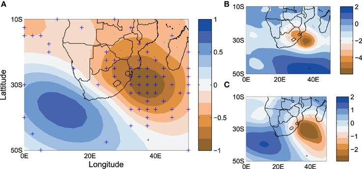
Figure 7. (A) Average anomaly pattern CP03 with (+) symbols indicating the centers of all negative anomalies (low pressures) contributing to the class. (B,C) show actual CP's for the dates 19/03/2007 and 30/08/2006, respectively, both of which were classified as members of the CP03 class.

FIGURE 8

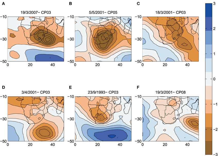
Figure 8. CP's associated with the six largest significant wave heights for the dates (A) 19/3/2007, (B) 5/5/2001, (C) 18/3/2001, (D) 3/4/2001, (E) 23/9/1993, and (F) 19/3/2001.

5. Discussion and Conclusions

In this paper different problems related to the fuzzy rule based classification of CPs were discussed. It was shown that reasonable classifications can be developed for precipitation and waves in South Africa. We did this by selecting long sequences of CPs in the region surrounding Southern Africa and conditioning the selection of the CPs on selected variables germane to the task; daily wetness for rainfall and wave height frequencies of ocean waves. The classifications yield classes with significantly different behavior depending on the classification goal. It was shown in the precipitation part of the study, that using different stations of a climatic region for the classification objective leads to different classifications, but the performance of these classifications is nevertheless very similar. Different classifications for the same region are more similar than classifications corresponding to different regions. This justifies the use of different classifications for the different regions and variables, because they add discriminatory power to the modeling procedure.

In the case of the wave study, the emphasis was on the statistical link between atmospheric CPs and extreme wave events. The results show that the classification algorithm is able to identify CPs that drive extreme wave events along the KZN coastline. The most frequent CPs associated with wave generation are revealed as low and high pressure anomalies south of the country. These reflect easterly traversing mid-latitude cyclones and their associated high pressures anomalies. The CP class that drives the majority of extreme wave events (labeled CP03) is associated with strong low pressure anomalies east of the country. A high/low pressure coupling drives strong winds toward the coastline and generates large waves. It is not clear what weather regimes are associated with these events since both mid-latitude cyclones and cut-off lows may belong to the CP03 class depending on their location. The classification algorithm does not currently identify CP anomalies as part of an overall structure developing in space and time: each class could be a snapshot in the temporal evolution of (perhaps distinct) CPs. Therefore, a particular weather system may be associated with a number of classes during its development, which makes for added complexity and requires further research.

There are similarities in the CP classes driven by the two surface variables because in some instances they are linked to similar synoptic weather systems. However, there are also significant differences in the details of the pressure fields. These differences are expected because large ocean waves are typically generated over fetches of the order of thousands of kilometers far off shore, whereas some rainfall is generated by local atmospheric variables including temperature, humidity, wind speed, and radiation over the area of concern.

Conflict of Interest Statement

The authors declare that the research was conducted in the absence of any commercial or financial relationships that could be construed as a potential conflict of interest.

Acknowledgments

Research leading to this paper was partly supported by the DFG, project number Ba-1150/18-1.

References

Bárdossy, A., Duckstein, L., and I, I. B. (1995). Fuzzy rule - based classification of atmospheric circulation patterns. Int. J. Clim. 15, 1087–1097.

Google Scholar

Bárdossy, A., Stehlik, J., and Caspary, H.-J. (2002). Automated objective classification of daily circulation patterns for precipitation and temperature downscaling based on optimized fuzzy rules. Clim. Res. 23, 11–22. doi: 10.3354/cr023011

CrossRef Full Text | Google Scholar

Corbella, S., and Stretch, D. (2012a). Predicting coastal erosion trends using non-stationary statistics and process-based models. Coast. Eng. 70, 40–49. doi: 10.1016/j.coastaleng.2012.06.004

CrossRef Full Text | Google Scholar

Corbella, S., and Stretch, D. (2012b). Shoreline recovery from storms on the east coast of South Africa. Nat. Hazards Earth Syst. Sci. 12, 11–22. doi: 10.5194/nhess-12-11-2012

CrossRef Full Text | Google Scholar

Corbella, S., and Stretch, D. D. (2012c). The wave climate on the the KwaZulu Natal coast. J. S. Afr. Inst. Civ. Eng. 54, 45–54.

Google Scholar

Corbella, S., and Stretch, D. D. (2013). Simulating a multivariate sea storm using Archimedean copulas. Coast. Eng. 76, 68–78. doi: 10.1016/j.coastaleng.2013.01.011

CrossRef Full Text | Google Scholar

Dee, D., Uppala, S., Simmons, A., Berrisford, P., Poli, P., Kobayashi, S., et al. (2011). The era-interim reanalysis: configuration and performance of the data assimilation system. Q. J. R. Meteorol. Soc. 137, 553–597. doi: 10.1002/qj.828

CrossRef Full Text | Google Scholar

Hartung, J., Bärbel, E., and Klösener, K. (2005). Statistik. München: Oldenburg Verlag.

Hess, P., and Brezowsky, H. (1952). Katalog der Großwetterlagen Europas. Bad Kissingen: Ber. DT. Wetterd. in der US-Zone 33.

Hewitson, B., and Crane, R. (2002). Self-organizing maps: applications to synoptic climatology. Clim. Res. 22, 13–26. doi: 10.3354/cr022013

CrossRef Full Text | Google Scholar

Jacobeit, J. (2010). Classifications in climate research. Phys. Chem. Earth A/B/C 35, 411–421. doi: 10.1016/j.pce.2009.11.010

CrossRef Full Text | Google Scholar

Kruger, A. C. (2004). Climate of South Africa: Climate Regions. Technical Report WS45, South African Weather Service, Pretoria.

Lamb, H. H. (1972). British Isles Weather Types and a Register of the Daily Sequence of Circulation Patterns, 1861–1971. London: HMSO; Meteorological Office. Geophysical Memoir No. 116.

Mather, A., and Stretch, D. (2012). A perspective on sea level rise and coastal storm surge from southern and eastern africa: a case study near Durban, South Africa. Water 4, 237–259. doi: 10.3390/w4010237

CrossRef Full Text | Google Scholar

Philipp, A., Beck, C., Huth, R., and Jacobeit, J. (2014). Development and comparison of circulation type classifications using the cost 733 dataset and software. Int. J. Climatol. doi: 10.1002/joc.3920. [Epub ahead of print].

CrossRef Full Text | Google Scholar

Preston-Whyte, R. A., and Tyson, P. D. (1988). The Atmosphere and Weather of Southern Africa. Cape Town: Oxford University Press.

Google Scholar

Pringle, J., Stretch, D., and Bardossy, A. (2014). Automated classification of the atmospheric circulation patterns that drive regional wave climates. Nat. Hazards Earth Syst. Sci. 14, 2145–2155. doi: 10.5194/nhess-14-2145-2014

CrossRef Full Text | Google Scholar

Rossouw, J., Coetzee, L. W., and Visser, C. J. (1982). “A South African wave climate study,” in IPCC. 18, 87–107. doi: 10.9753/icce.v18.%25p

CrossRef Full Text