Impact of Land Surface Initialization and Land-Atmosphere Coupling on the Prediction of the Indian Summer Monsoon with the CFSv2

Introduction

Does land surface initialization matter for the forecast of the Indian summer monsoon rainfall (ISMR) and temperature on sub-seasonal to seasonal time scales? That is the question being addressed. Though state-of-the-art dynamical models have demonstrated improvement in the prediction skill of the ISMR in the last decade (Kumar et al., 2005; DelSole and Shukla, 2012; Kim et al., 2012; Rajeevan et al., 2012; Nanjundiah et al., 2013; Sperber et al., 2013), much of the skill has derived from improved forecasts of sea surface temperature (SST) (DelSole and Shukla, 2012), and the strong relationship that the ISMR bears with SST over different ocean basins (Saji et al., 1999; Gadgil et al., 2003; Goswami et al., 2006; Kumar et al., 2006). However, it is still much less than the potentially achievable skill (Rajeevan et al., 2012; Goswami and Chakravorty, 2017). Anomalies in soil moisture and snow at the land surface, which vary on low-frequency time scales, can also affect the atmosphere from weeks to months (Charney et al., 1975; Shukla and Mintz, 1982; Koster and Suarez, 1995, 2004; Ashfaq et al., 2017) and are a source of predictability (Shukla, 1985; Koster et al., 2004; Dirmeyer, 2006; Guo et al., 2012) beyond the deterministic limit for weather forecasts (Dirmeyer et al., 2009). Therefore, the next frontier for improvement in the Indian summer monsoon prediction is the land surface.

The central and northwestern parts of India constitute one of the global “hot spots” of land-atmosphere coupling where soil moisture anomalies exert a significant control on temperature and precipitation via strongly coupled processes (Koster et al., 2004; Guo et al., 2006; Dirmeyer, 2011; Halder et al., 2015). In addition, efforts to investigate the role of land-surface processes during the onset (Saha et al., 2011, 2017; Bollasina and Ming, 2013; Senan et al., 2016) and in the low-frequency variability of the Indian summer monsoon (Webster, 1983; Ferranti et al., 1999; Yasunari, 2007; Turner and Slingo, 2011; Saha et al., 2012; Halder et al., 2015, 2016; Halder and Dirmeyer, 2017) have further added to the confidence that the prediction skill of the Indian summer monsoon can be further improved. However, the actual prediction skill arising from anomalies in the land surface state may depend on the methods of forecast initialization (Dirmeyer, 2005; Koster et al., 2011), errors in land surface initial conditions (Dirmeyer and Halder, 2016, 2017) and the systematic errors in the model (Dirmeyer, 2003) that affect the land-atmosphere (LA) coupling strength (cf. Halder et al., 2015). Therefore, it behooves us further investigation from the perspective of the land surface, particularly in the Climate Forecast System version 2 model (CFSv2; Saha et al., 2014) that is used for routine operational forecasts by the India Meteorological Department (IMD).

Within the framework of the Global Land Atmosphere Coupling Experiment version 2 (GLACE2), several global models were able to demonstrate improvement in the hindcast prediction skill due to realistic, observationally-based land surface initialization (Koster et al., 2010, 2011). However, the Global Forecast System version 2 (GFSv2), the atmospheric component of the CFSv2 was unable to show any improvement due to its inherent weaknesses in the representation of LA feedbacks (Wei and Dirmeyer, 2010; Guo et al., 2011, 2012; Zhang et al., 2011). Dirmeyer (2013) demonstrated that despite evidence of evaporation-soil moisture feedback in CFSv2 that is essential for land driven predictability, the atmospheric component did not appear to maintain the necessary linkage between antecedent soil moisture and precipitation. Therefore, understanding the attribution of the processes responsible for such weakness and their impact on the prediction skill in CFSv2 over the monsoon region is foremost necessary. In this context, Yang et al. (2011), Dirmeyer and Halder (2016, 2017), Halder and Dirmeyer (2017), and Saha et al. (2017) have discussed a range of systematic biases in CFSv2 that are attributable to land surface processes. Although prediction skill of the Indian summer monsoon on different time scales by the CFS model was earlier evaluated (Rai and Krishnamurthy, 2011; Pokhrel et al., 2015; Sahai et al., 2015; Ramu et al., 2016), a systematic investigation of the impact of land surface initialization and LA coupling on the skill was lacking. Therefore, the following objectives are addressed in this study: (1) Characterize land-atmosphere feedback mechanisms over the Indian summer monsoon region on sub-seasonal (i.e., monthly) to seasonal time scales, (2) quantify the potential predictability and prediction skill of the model due to land surface initial conditions, and (3) understand the impact of biases in the representation of land-atmosphere coupling on the prediction skill.

The model and the data used for validation of the model are presented in section Model and Data. Section Experiments describes the experiment design and methodology. Metrics of land-atmosphere coupling and skill scores are discussed in this section. Results discussed in third section are grouped under two broad categories: understanding coupled land-atmosphere feedbacks during the monsoon season and secondly, impact on the predictability and prediction skill. Section discussion explores the possible mechanisms and summarizes the results.

Model and Data

Model

The atmospheric component of CFSv2, the GFSv2 has a horizontal resolution of ~0.9° (T126 spectral resolution) whereas the coupled Modular Ocean Model version 4 (MOM4; Griffies et al., 2004) has a horizontal resolution of 1/2°, increasing further to 1/4° in the meridional dimension near the equator. Vertical levels used are 64 in the atmosphere (topmost level reaching up to 0.2 hPa) and 40 in the ocean. Sea ice is predicted using a modified version of the Geophysical Fluid Dynamics Laboratory (GFDL) Sea Ice Simulator (cf. Saha et al., 2010). The land surface model coupled to GFSv2 is Noah version 2.7.1 (Ek et al., 2003) having four soil layers; the individual layers starting from the surface have depths of 10, 40 cm, 1, and 2 m respectively. Noah calculates the surface energy and water budgets and estimates the transpiration component of evapotranspiration based on plant water stresses.

Along with the planetary boundary layer scheme from Hong and Pan (1996), an additional background vertical diffusion term is included for enhanced mixing close to the surface e.g., in stable regimes when the eddy diffusion calculated by the PBL scheme is insufficient. A shallow convection scheme (Tiedtke, 1983) is used in locations where deep convective parameterization is not active. The Rapid Radiative Transfer Model (RRTM; Mlawer et al., 1997; Clough et al., 2005) radiation scheme is the same as that used to generate the CFS reanalysis (CFSR; Saha et al., 2010) but with major differences in cloud-radiation calculation. A Monte Carlo independent column approximation (McICA) (Barker et al., 2002; Pincus et al., 2003) is used for addressing the unresolved variability of layered clouds in fractionally cloud covered model grids.

Validation Data

Daily high-resolution (0.5 × 0.5°) gauge-based rainfall from the Climate Prediction Centre CPCv1.1 (in short CPC; Chen et al., 2008) is averaged into monthly values and then blended with the Global Precipitation and Climatology Project GPCPv2.2 (in short GPCP; Adler et al., 2003) combined satellite and gauge based monthly data (2.5 × 2.5°) over land by giving equal weightage to both (together CPC/GPCP), for the validation of model output and calculation of skill metrics. For 2 m near surface air temperature, monthly data (0.5 × 0.5°) from the Climate Research Unit CRU TS v3.21 (in short CRU; Harris et al., 2014) is used for validation and assessment of skill metrics. Additionally, daily surface temperature data (1 × 1°; 1982–2005) from the India Meteorological Department (IMD; Srivastava et al., 2009) averaged into monthly values is also used in place of CRU data over the Indian region for the comparison of skill scores. For the verification of state variables simulated over land, the Global Land Data Assimilation System version 2.0 (GLDAS2; Rodell et al., 2004) based daily soil moisture [surface (0–10 cm) and sub-surface (10–40 cm)] analyses (1 × 1°) are used. In addition, daily near surface state variables, fluxes, and diagnostics from the CFSR at T382 resolution (~38 km) and the Modern-Era Retrospective analysis for Research and Applications, Version 2 (MERRA2; Gelaro et al., 2017) at 0.625 × 0.5° resolution are used for the assessment of land-atmosphere coupling strength. Surface short wave (v3.0) and longwave (v3.1) 3-h radiation fluxes from the Surface Radiation Budget experiment (SRB, Stackhouse and Gupta, 2013) are converted to daily and monthly values in order to validate the net radiation simulated by the model. All the data are re-gridded to a common spatial resolution (that of the CFSv2) before the calculation of biases, skill metrics, and coupling diagnostics.

Experiments

Model Initialization and Hindcasts

Model simulations are initialized with the CFSR that has a higher horizontal resolution (T382, ~38 km) but also 64 vertical levels in the atmosphere (Saha et al., 2010). The sea surface temperature (SST) analysis for the ocean in CFSR uses two daily SST analyses at 1/4° developed using an optimum interpolation scheme. The first is an AVHRR-only SST data set (November 1981 through May 2002) and the second is a combined AMSR+AVHRR SST data set from June 2002 onwards (Reynolds et al., 2007). Assimilated sea ice concentrations are derived from several data sets (Cavalieri et al., 1996, 2007; Grumbine, 1996; Saha et al., 2010). It is important to note that the land states in CFSR are reset every 24 h at 0000UTC from a parallel offline simulation of Noah v2.7.1 using atmospheric forcing from the GFS data assimilation system (GDAS) and precipitation based on a blend of observed global analyses (Xie and Arkin, 1997; Xie et al., 2007) and the 6-h precipitation generated by GFSv2. Thus, the land surface model is said to be “semi-coupled” to the atmosphere in CFSR. Such observational data-driven land surface analyses, offline, or semi-coupled, where the errors of an atmospheric model are not included, can provide the best estimate of land-atmosphere coupling strength where there is lack of availability of long-term, high-resolution micrometeorological surface flux observations.

Ensemble hindcasts are built around perturbations in land initial conditions that are achieved in the following way. Hindcast simulations are performed for the period spanning 1982–2009; in each year three sets of 28-member ensembles are generated by initializing the model at 0000UTC on the 1st of April, May, and June and running through 0000UTC on the 1st of October. For a particular initial date, the Control run (baseline ensemble member) is initialized from CFSR for that date. The remaining 27 ensemble members are initialized with the same atmosphere, sea ice and ocean states as in the Control simulation, but with initial land states taken from each of the remaining 27 years to span the interannual variability and achieve maximum initial land perturbation. In other words, one member (Control run) has the “correct” land initial state consistent with the atmosphere, sea ice and ocean states for that year, and the other 27 members effectively have “incorrect” land states. We name these initial states as “realistic” and “randomized” land initial conditions (ICs), respectively.

Assessment and Validation Methodology

Land-atmospheric coupling takes place via two legs or steps; the “terrestrial” leg that determines when and where soil moisture anomalies strongly affect surface fluxes of moisture and sensible heat (Dirmeyer, 2011) and secondly, the “atmospheric” leg that governs when and where variations in surface fluxes strongly affect the near surface atmospheric variables such as temperature and humidity, and growth of the boundary layer (Dirmeyer et al., 2014) up to the lifting condensation level (LCL) eventually leading to moist convection, formation of clouds, and precipitation. LA coupling is said to exist if both the legs are strong and in place over a region (Dirmeyer et al., 2014). Locations where the water or the energy cycle would be the preferred pathway of coupling depends on the climate regime and season (Findell and Eltahir, 2003a,b).

Coupling strength in the model is analyzed following the modern paradigm of land-atmosphere coupling. It proposes that all three components, namely adequate sensitivity of the atmosphere to variations in fluxes and soil moisture at the land surface, sufficient magnitude of those land surface variations and persistence of the anomalies represented in those variations (a.k.a. memory), should be prevalent over a region for it to be a location of strong land-atmosphere coupling. Sensitivity that is quantified using correlation (implying covariability) is based on actual physical processes or causality (Dirmeyer, 2011) and is an important metric widely used to quantify land-atmosphere coupling (cf. Dirmeyer and Halder, 2016, 2017; Hirsch et al., 2016; Lorenz et al., 2016; Draper et al., 2017; Halder and Dirmeyer, 2017). The important aspect of this metric is that while accounting for standard deviation along with correlation, it rules out the possibility of LA coupling over those regions where there is high correlation between two variables but low variability. For example, places showing significant positive (negative) correlation between soil moisture and evapotranspiration (sensible heat) suggest the presence of sensitivity whereby the fluxes are strongly controlled by soil moisture variations. This means evapotranspiration in those regions that are more specifically termed as “hot-spots” of land-atmosphere coupling (Koster et al., 2004), is limited by soil moisture availability. Places showing the opposite correlation indicate that it is not soil moisture but other factors such as surface net radiation or atmospheric moisture demand that are in control. However, in certain other regimes such as hot deserts with ample surface net radiation, weak soil moisture variability can limit coupling despite presence of strong correlations. Last but not the least, soil moisture memory, which allows sensitivity and variability time to manifest into climate anomalies via LA feedbacks, is calculated on the basis of daily autocorrelations for each ensemble member (cf. Dirmeyer et al., 2016).

The indices' variability (i.e., standard deviation denoted by σ) and sensitivity when combined together result into the terrestrial coupling index (TCI; Dirmeyer, 2011) or the atmospheric coupling index (ACI; Dirmeyer et al., 2014). The TCI is formulated as

$\begin{array}{ll}TCI={\sigma }_{F}Cor{r}_{FL}& (1)\end{array}$

where, F represents surface latent or sensible heat flux (LHF or SHF) and $Cor{r}_{F^L}$ represents the correlation between a land state such as surface or root zone soil wetness (SSW or RSW, represented by L) and those fluxes (i.e., F). On the other hand, the ACI is formulated as

$\begin{array}{ll}ACI={\sigma }_A{Corr}_{AF}& (2)\end{array}$

where, A represents atmospheric variables such as 2 m air temperature (2 mT), specific humidity (2 mQ) or diagnostics such as the planetary boundary layer (PBL) height, lifting condensation level (LCL) height or total cloud cover (TCC), and F represents the fluxes of moisture or heat. Only correlations between A or L and F significant at the 99% confidence level are considered.

We characterize the predictability and prediction skill of the model on monthly and seasonal (JJAS) time scales. Potential predictability of a particular variable “x_en” is quantified using the ratio of its signal to total variance across the ensemble members with perturbed land or atmosphere/ocean ICs. Following Shukla et al. (2000), the total climatological variance of the variable x_en across forecasts initialized in a particular month is given as:

$\begin{array}{ll}{V}_T=\frac{1}{NE}{\displaystyle \sum _{n=1}^N}{\displaystyle \sum _{e=1}^E}{(x_{en}-\overline{\overline{x}})}^2& (3)\end{array}$

Here, N and E stand for the total number of years of validation and ensemble members respectively. The, grand and ensemble mean are respectively defined as:

$\begin{array}{ll}\overline{\overline{x}}=\frac{1}{NE}{\displaystyle \sum _{n=1}^N}{\displaystyle \sum _{e=1}^E}{x}_{en},\text{and }\overline{x}=\frac{1}{E}{\displaystyle \sum _{e=1}^E}{x}_{en}& (4)\end{array}$

Total variance can be decomposed into two parts: the variance of ensemble means across the different initial states for the same month of different years (signal):

$\begin{array}{ll}{V}_s=\frac{1}{N}{\displaystyle \sum _{n=1}^N}{(x_{en}-\overline{\overline{x}})}^2& (5)\end{array}$

and the variance of individual ensemble members about their corresponding ensemble means (noise):

$\begin{array}{ll}{V}_N=\frac{1}{NE}{\displaystyle \sum _{n=1}^N}{\displaystyle \sum _{e=1}^E}{(x_{en}-\overline{x_n})}^2& (6)\end{array}$

By suitably grouping the simulations whereby 28 different atmosphere/ocean ICs pertain to ensemble members for a particular land IC, we can quantify the predictability and prediction skill due to initial land states. While validating the forecasts against observation, for each initial start month, Control simulations with “realistic” land ICs (hereafter RealLIC) are considered as one set for purposes of estimating interannual anomaly correlation coefficients, root-mean-square-error (RMSE) and mean absolute bias (MAB) as measures of skill. Remaining 27 ensemble members with “randomized” land ICs (hereafter RandLIC) but same atmospheric/ocean ICs are used for comparison. Significance of the signal-to-total variance ratio (predictability) is tested following a slightly modified Fischer's F-test (cf. Guo et al., 2011), under the null hypothesis of no predictability. For testing the significance of correlations, difference in means and land-atmosphere coupling metrics, a Student's t-test is used.

Results

Modeled Climate during the Indian Summer Monsoon Season

Simulated precipitation statistics during the monsoon season (JJAS) with April, May, and June initial conditions (in short, APRIC, MAYIC, JUNIC) are validated against observations (Figure 1) to explore the fidelity of the model. For that we shall mainly concentrate on the JUNIC seasonal hindcasts (Figure 1a), but use all the three sets for characterizing monthly evolution of forecasted variables with the lead-time. The observed spatial pattern of rainfall is reasonably well simulated, particularly the regions of rainfall maxima over the Western Ghats (WG) orography and adjoining Arabian Sea (AS), central India (CI), the head Bay of Bengal (BoB) and northeastern states, and foothills of the Himalayas (Figure 1b). Such regions also depict high interannual standard deviation, although it appears much stronger in the model (Figure 1d) than observations (Figure 1e). Differences (Figure 1c) further suggest an underestimation of seasonal rainfall by the model over land, particularly CI and the northwest, as reported in earlier studies (cf. Ramu et al., 2016). On the contrary, there is an overestimation of rainfall over the Himalayan region, eastern and northeastern states, and the oceanic region. Differences also reveal higher interannual variability over CI and the Indian Ocean, except over the northwest and the Indo-Gangetic plains to the north (Figure 1f).

FIGURE 1

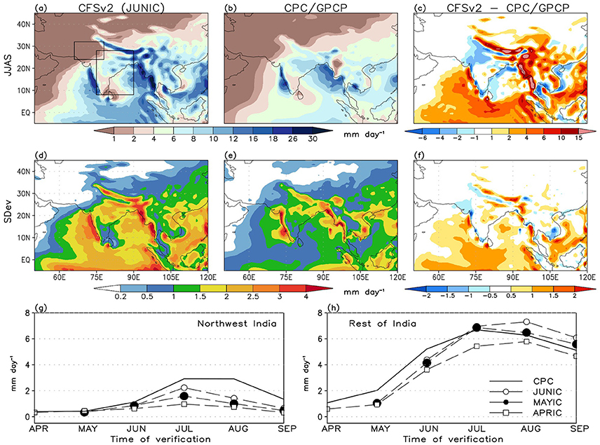
Figure 1. Mean (1982–2009) seasonal (JJAS) precipitation from (a) CFSv2 JUNIC hindcasts and (d) its interannual standard deviation (SDev). (b,e), respectively show the same for CPC/GPCP2 combined observations. Rightmost column shows differences in (c) seasonal mean and (f) SDev. Units are mm day⁻¹. Bottom row shows monthly precipitation over the (g) northwest and (h) rest of India domains as depicted by small and big boxes in the first panel; for JUNIC, MAYIC, and APRIC hindcasts and observations.

On further examination of monthly rainfall from April through September, it emerges that the northwest India (NWI) region remains perennially drier in the model than observation (Figure 1g) with the dry bias increasing with the forecast lead-time (cf. Dirmeyer, 2013). This evolutionary feature of dry bias is true for the rest of India (ROI) as well, although forecasts initialized in May appear to follow the observed monthly seasonal cycle the best (Figure 1h). All the forecasts fail to capture rainfall over land realistically during the onset period i.e., May–June; and for forecasts initialized in June, the rainfall is overestimated toward the end of the season.

Soil moisture is a principal component of the hydrologic cycle that controls the partitioning of surface net radiation into sensible and latent heat fluxes that affect near surface meteorological parameters and evolution of the boundary layer. The climatological pattern of simulated (Figure 2a) and observed (Figure 2b) soil moisture in the top 1 m basically follows that of precipitation, except that the eastern and northern parts of CI appear to be drier than expected. The model soil layers are relatively drier toward the north, northwest, and peninsular India compared to the other regions, which could be due to below normal precipitation. The climatological spatial pattern is comparable to that of GLDAS2. However, simulated soil moisture appears higher than observed over the Himalayas and adjoining Tibet, and eastern and northeastern parts of India. Almost the entire Indian land part has a systematic negative bias in simulated soil moisture, except over the Himalayan region and the northeast (Figure 2c). We verify that the interannual variability of simulated soil moisture is also much stronger compared to the observed analysis almost all over India (Figures 2d–f) except over the north, northwest and northeastern regions. Simulated monthly soil moisture also depicts that the systematic dry bias over the ROI domain that aggravates with the forecast lead-time from June to April (Figure 2h). Over NWI, the biases are starkly negative in most of the months (Figure 2g). Such biases have important implications for coupled model based forecasts for the agriculture and hydrologic sectors.

FIGURE 2

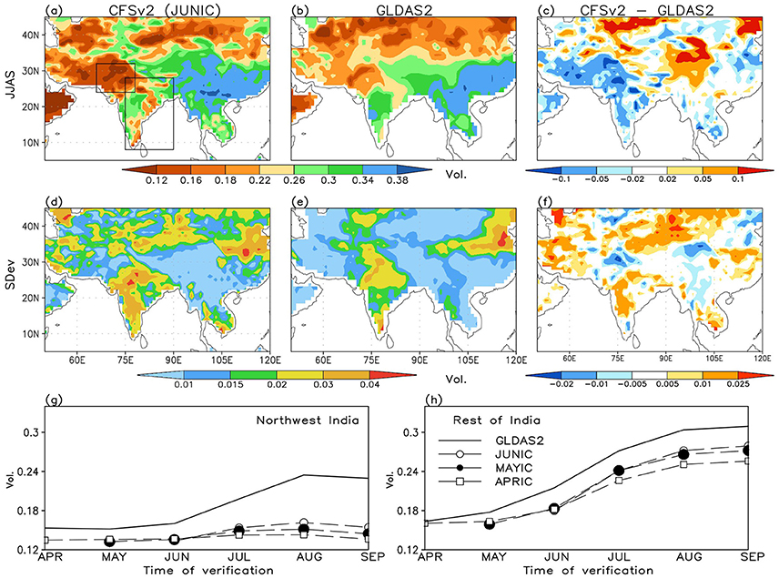
Figure 2. Same as in Figure 1, except for top 1 m soil moisture. Observations are from the GLDAS2. Units are volumetric.

Simulated monthly and seasonal 2 m air temperature are overestimated over the relatively dry NWI, northern and eastern parts of CI during the summer monsoon, but is relatively underestimated over peninsular India and the northeastern states (Figures 3a–c). Lowest surface temperatures are simulated over the Himalayas and adjoining Tibet on account of higher altitude, and northeastern states. A part of these differences maybe attributed to the dry precipitation bias; rather biases in the simulation of clouds (Bombardi et al., 2015) and surface net radiation (cf. Halder et al., 2015) are also largely responsible. Interannual variability of the simulated temperature is also overestimated over central India (Figures 3d–f). However, farther west over the arid and cloud free areas near Afghanisthan and Iran, the surface temperature variability is much subdued and maybe attributed to biases in the radiation scheme or the representation of aerosols in the model. The monthly evolution pattern of simulated surface air temperature over NWI does not reveal many differences among the three forecast sets; almost all of them overestimate it by about 1–2°C before and during the season (Figure 3g). On the contrary, performance of the monthly forecasts over the ROI is relatively better in terms of the bias (Figure 3h). Once again, the MAYIC forecasts appear to be the best among all three, particularly after June.

FIGURE 3

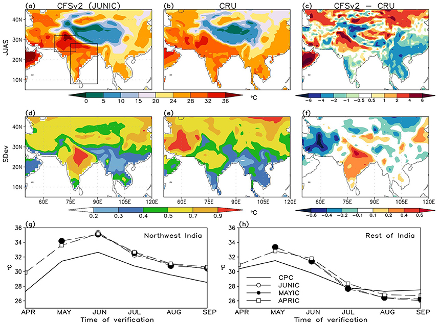
Figure 3. Same as in Figure 1, except for 2 m air temperature. Observations are from the CRU. Units are in °C.

The Modern Land-Atmosphere Coupling Paradigm Applied to CFSv2

Sensitivity

As aforementioned, one of the prime metrics of land-atmosphere coupling is sensitivity. We analyze the sensitivity (through correlation) of surface fluxes (LHF, SHF) to surface soil wetness (SSW) at first, followed by that of the planetary boundary layer (PBL) height and total cloud cover (TCC) to the surface fluxes. In general, LHF is positively correlated to SSW over India during JJAS implying that surface evapotranspiration is strongly limited by soil moisture variations (Figure 4a), whereas for SHF it is just the opposite (Figure 4b). As in CFSR (Figures 4e,f), the free running model initialized in June captures the spatial pattern of correlations in JJAS very well although, it is apparent that LHF is weakly (strongly) sensitive to SSW variations over the NWI (ROI) region. For SHF, sensitivity over the northwest region is weaker than observations but matches reasonably well for the rest of India. Sub-seasonal (monthly) evolution features also suggest that the terrestrial coupling strength for both LHF (Figures 4i,m) and SHF (Figures 4j,n) are weaker in CFSv2 than CFSR. The differences in sensitivity are much stark during July to September.

FIGURE 4

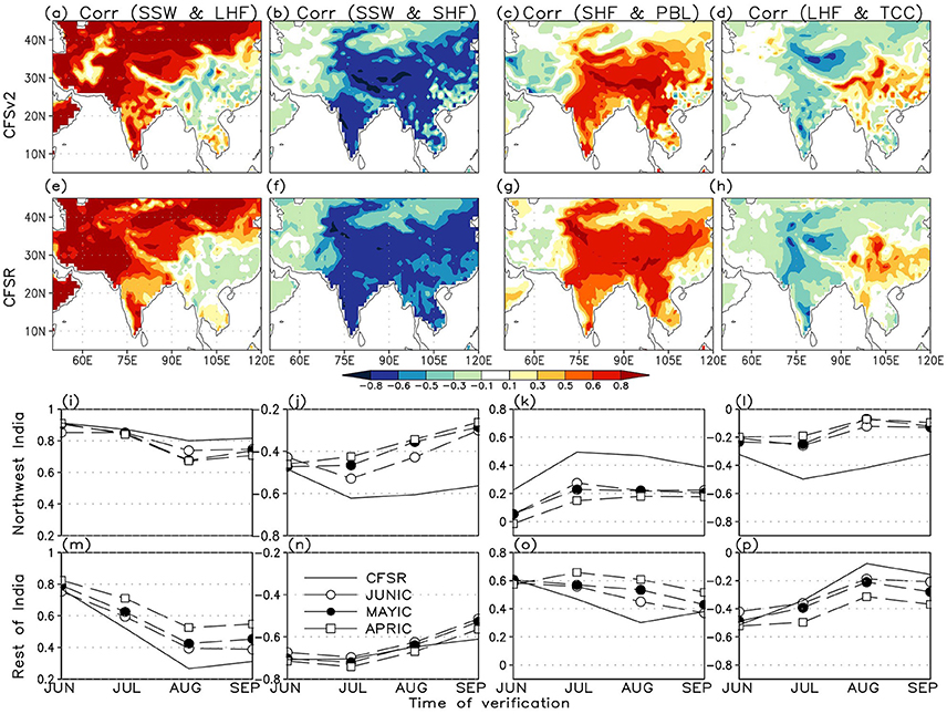
Figure 4. Ensemble-mean correlation of daily SSW with (a) LHF and (b) SHF; and (c) SHF with PBL height, and (d) LHF with TCC in JJAS from CFSv2 JUNIC hindcasts. (e–h) respectively, show similar correlations based on the CFSR. (i–p) show monthly correlations for the same variables for the northwest and rest of India domains, respectively; from JUNIC, MAYIC, and APRIC hindcasts and CFSR.

The sensitivity of near surface/boundary layer variables and convection to the fluxes of heat and moisture i.e., the atmospheric leg, are further evaluated. For PBL height, strongly positive correlations over India, the Himalayas and adjoining Tibet, and the areas further east (Figure 4c) imply a strong control of SHF on the boundary layer growth. Weaker correlations over the WGs and northwest, eastern parts of CI and peninsular India imply that chances of convective initiation happening through the moisture pathway maybe comparatively higher. Figure 4g shows that the correlations in CFSv2 JUNIC runs are much weaker over the northwest and east CI. On the other hand, negative correlations of TCC with LHF (Figure 4d) indicate a plausible greater control of surface net radiation (NRAD). Increased cloud-cover during the monsoon season cuts-off NRAD, leading to decrease in surface moisture fluxes. Such impacts appear to be very weak over east CI that is already in a wet regime during JJAS. However, the dependence of surface evapotranspiration on the availability of NRAD is not as strong in CFSv2 over NWI as in observations (Figure 4h); suggesting the climate in that region is in a relatively drier regime. Monthly correlations also depict weaker terrestrial coupling in CFSv2 (Figures 4k,l) compared to the observations (Figures 4o,p), for both PBL height and TCC; with more realistic coupling in June. Furthermore, the JUNIC runs perform the best in terms of capturing the coupling strength on the sub-seasonal time scale.

Variability

Daily variability in surface and root zone soil wetness is mostly high over the western parts of CI, north and peninsular India; whereas the wet and humid northeastern states and adjoining Himalayas and arid deserts to the west depict very low variations (Figures 5a,b). Soil moisture variability gets subdued i.e., frequency tends to become more red as we explore further deep into the soil layers. We notice lower (higher) variability captured by the coupled model as compared to observations (Figures 5e,f) over the northwest and north India (CI and the peninsula). Differences indicate at shortcomings in the correct representation of daily precipitation variability in the model (cf. Bombardi et al., 2015). Such biases in turn can affect persistence in soil moisture anomalies also. Furthermore, uncertainty in the representation in snow cover and related hydrology is also evident from the differences over the Himalayas; a common systematic error noted in many models (Tiwari et al., 2016; Ashfaq et al., 2017).

FIGURE 5

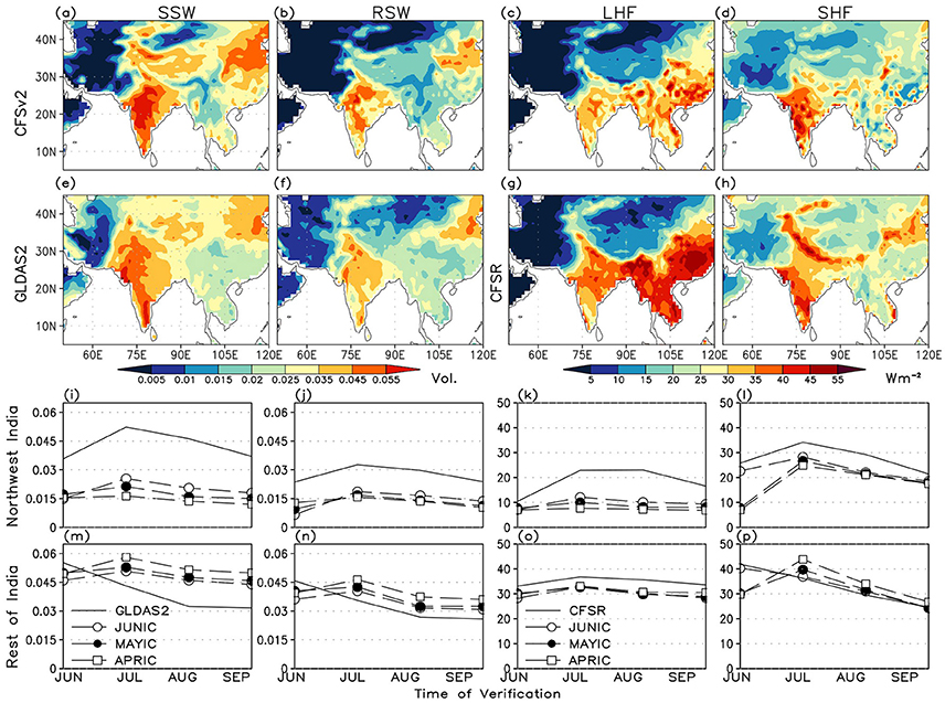
Figure 5. Ensemble-mean daily variability of (a) SSW, (b) RSW, (c) LHF, and (d) SHF in JJAS for CFSv2 JUNIC hindcasts. Observed variability of (e) SSW and (f) RSW are based on GLDAS2 whereas that of (g) LHF and (h) SHF are based on CFSR. Units of variability for soil wetness are Volumetric and Wm⁻² for fluxes. (i–p) show the daily variability in different months for the northwest and rest of India domains, respectively; from JUNIC, MAYIC, and APRIC hindcasts and for GLDAS2 and CFSR.

Observed daily variability in surface LHF depicted in CFSR is well-captured by the free running model, except over NWI, northern parts and adjoining Himalayas (Figures 5c,g). However, the magnitude of LHF variability simulated in the model is much subdued. Variability in SHF appears to be better captured over the western and peninsular India in terms of magnitude (Figures 5d,h). However, the free running model grossly overestimates (underestimates) the observed SHF variability over CI (north India and the entire Himalayan belt). Stark contrasts are also verified over the Tibet and the arid regions further west. The monthly evolution of observed soil moisture and surface fluxes over northwest India depicts a peak in June and July followed by a decline that is aptly captured by CFSv2 (Figures 5i–l). The free running model however, fails to capture the monthly evolutionary feature over ROI (Figures 5m–p). Despite the biases, JUNIC hindcasts are the closest to CFSR among all three. Such biases in the correct estimation of daily variability of surface fluxes and soil moisture can affect the terrestrial and atmospheric legs of land-atmosphere coupling in the model, as suggested by equations (1, 2).

It is verified that the mean surface NRAD and its daily variability (Figures 6a,b) during JJAS are not realistically captured in CFSv2 when compared to observations from the SRB (Figures 6c,d). The spatial pattern of simulated daily variability in NRAD appears to follow that of mean seasonal precipitation over India that suggests it might be associated with the spatial distribution of clouds as well. Highly overestimated surface NRAD over the Indian land part contributes to the positive bias in simulated surface SHF mostly over the north and NWI where the simulated soil moisture is also low (Figure 6e). This is partly the reason why there is a positive surface temperature bias over that area. On the contrary, surface NRAD is much underestimated over the Himalayan region, adjoining Tibet, and the Arabian Sea. Daily NRAD variability is higher than that observed over CI, northeast and the Himalayas, but lower over the Indo-Gangetic plains, western Himalayas, and NWI (Figure 6f). Such differences could be attributed to systematic errors in the correct simulation of the vertical distribution of clouds (Bombardi et al., 2015), radiation and atmospheric humidity (Goswami et al., 2017), representation of aerosols and surface albedo. Similarity among these and the pattern of differences in surface heat and moisture fluxes suggests how the latter could be strongly affected by NRAD errors over the Indian region leading to biases in the representation of LA coupling.

FIGURE 6

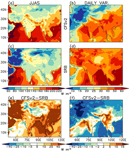
Figure 6. Mean (1982–2009) seasonal (JJAS) surface NRAD based on (a) ensemble mean JUNIC hindcasts and (b) observations from the SRB project. (c,d) Show the same except for the daily variability in NRAD in JJAS. Differences in the (e) seasonal mean and (f) daily variability of NRAD between the JUNIC hindcasts and SRB are shown in the bottom row. Units are in Wm⁻².

Land-Atmosphere Coupling

A combination of sensitivity and variability results in the terrestrial and atmospheric coupling indices (TCI and ACI; Equations 1, 2). As a result of the systematic errors in net radiation, surface fluxes, and soil moisture, weaker than observed TCIs and ACIs for 2 m specific humidity (2 mQ) and LCL height are depicted by CFSv2 over India during JJAS (Figures 7a–f), particularly over NWI and western and northern parts of CI. This could be a plausible reason why convective activities leading to rainfall are lesser over those areas compared to CI, despite having strong positive bias in surface temperature. Here, both CFSR and MERRA2 (shown in black contours) data are used to quantify LA coupling over the Indian region. We note that the terrestrial leg of LA-coupling for near surface humidity is not in place over east CI as the land surface is already in a wet regime. On monthly time scales the model fails to capture the sub-seasonal evolution of LA coupling, particularly over NWI (Figures 7g–i), although the JUNIC hindcasts are closest to CFSR in this respect. It performs relatively better over the ROI (Figures 7j–l). It is further noted that, in general, the seasonal spatial distribution and monthly evolution of the coupling indices are similar for both CFSR and MERRA2 such that the sign of the errors in CFSv2 hindcasts are same w.r.t both reanalyses. However, there are some differences in terms of the TCI over NWI and ACI over the ROI that may be attributed to the differences between models and data assimilation schemes.

FIGURE 7

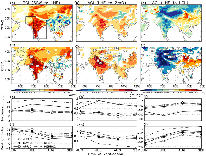
Figure 7. (a) Terrestrial coupling index (TCI) for 2 m specific humidity (2 mQ) based on SSW and LHF and (b) the corresponding atmospheric coupling index (ACI) based on LHF and 2 mQ, from CFSv2 JUNIC hindcasts. (c) shows the ACI for LCL height. Units are Wm⁻², gm Kg⁻¹, and m, respectively. (d–f) respectively, shows the same for CFSR (shaded) and MERRA2 (black contours). (g–i) and (j–l) show the monthly coupling indices in JJAS for the northwest and rest of India domains, respectively; from JUNIC, MAYIC and APRIC hindcasts, CFSR and MERRA2.

LA coupling in JJAS for 2 m air temperature and PBL height are also weakly represented in CFSv2 over the NWI and north (Figures 8a–c) when compared to observations (Figures 8d–f). This is also evident on monthly (sub-seasonal) time scales over the NWI (Figures 8g–i). For convenience, the terrestrial coupling index for SHF with the opposite sign is shown. Further, over east of CI it appears that LA coupling for PBL height is also not well-captured by the model. Over the ROI domain the terrestrial segment of coupling for SHF is stronger than both the reanalyses, although, the ACIs for both 2 mT and PBL height appear to be relatively well represented on sub-seasonal time scales as in observations (Figures 8j–l). Differences in the coupling strength between CFSv2 and observations that grow with the forecast lead-time are associated with systematic errors in cloudiness and rainfall, and NRAD and surface fluxes. Differences between CFSR and MERRA2 in terms of the coupling indices are apparent only over the ROI domain. Such differences shall be systematically investigated in future studies.

FIGURE 8

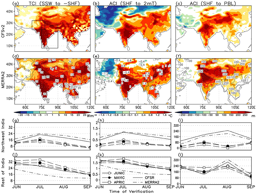
Figure 8. (a) Terrestrial coupling index (TCI) for 2 m temperature (2 mT) based on SSW and SHF and (b) the corresponding atmospheric coupling index (ACI) based on SHF and 2 mT from CFSv2 JUNIC hindcasts. (c) shows the ACI for PBL height. Units are Wm⁻², °C, and m, respectively. (d–f) respectively, shows the same for CFSR (shaded) and MERRA2 (black contours). (g–i) and (j–l) show the monthly coupling indices in JJAS for the northwest and rest of India domains, respectively; from JUNIC, MAYIC and APRIC hindcasts, CFSR and MERRA2.

Memory

Unless the anomalies in soil moisture over a region persist for sufficiently long time, variability in near surface and atmospheric variables brought about by the changes in surface fluxes will not sustain and transpire into a meaningful atmospheric response (Guo and Dirmeyer, under review). Over the Indian region, surface soil moisture memory in CFSv2 extends only up to about a week and gradually decreases from April (dry season) through June (monsoon onset period, Figures 9a,e,i). The arid region to the west of India has longer memory compared to the wet and humid regions to its east. Soil moisture anomalies in the root zone persist comparatively longer, particularly over the north and NWI (Figures 9b,f,j). The memory is about two months in April that decreases through June with increasing precipitation and soil wetness (for deeper layers it is closer to a season; not shown). Longer memory in the root zone and deeper layers can help in maintaining the initial soil moisture anomalies for substantially long periods and may affect the surface fluxes on sub-seasonal time scales. In general, soil moisture memory over ROI (drier areas of NWI) appears to be higher (lower) than that depicted in GLDAS2 (Figures 9c,d), which is mainly a result of differences in observed and simulated daily precipitation statistics. Furthermore, as the precipitation in June further decreases with the forecast lead-time (APRIC and MAYIC), an increase in the persistence of soil moisture anomalies over the west of CI, north and NWI becomes increasingly apparent (Figures 9g,h,k,l). Such changes in soil moisture memory and hence LA coupling can affect the forecast of near surface temperature and rainfall.

FIGURE 9

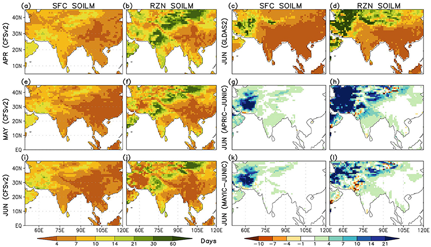
Figure 9. (a) Surface (SFC) and (b) root zone (RZN) soil moisture (SOILM) memory in April based on CFSv2 APRIC hindcasts. (e,f, i,j) show the same for May and June based on MAYIC and JUNIC hindcasts, reespectively. (c,d) shows the soil moisture memory in June based on GLDAS2. Changes in soil moisture memory in June based on (g,h) APRIC-JUNIC, and (k,l) MAYIC-JUNIC hindcasts Units are in days.

Predictability and Prediction Skill due to Land Surface Initialization

Potential Predictability

At the outset, there is very little potential predictability of precipitation in this model over the Indian region due to land initial conditions (not shown). Potential predictability due to ocean initial conditions however, persists throughout the boreal summer season, and is the strongest over the eastern Pacific Ocean (Supplementary Figure S1). Here, the first 30-day average has not been shown to exclude the effect of persistence in atmospheric ICs. For 2 m air temperature, potential predictability of the model attributed to land and ocean initial conditions is depicted (Figure 10) for 30-day average periods starting from the date of initialization in June and April. The ensembles are arranged in such a way that for a particular land initial condition the initial atmosphere/ocean states are randomized. The lowest shaded value corresponds to the 95% confidence level. Predictability of the model due to land initial conditions in June is notable only in the first month (Figure 10a), particularly over north and northwest India and adjoining Himalayas; east, northeast and southern Tibet, and the peninsula. Thereafter, it dissipates rapidly within the season (Figures 10b–d). For April (and May, figure not shown) initial conditions, land driven potential predictability is evident over areas more widespread than in June (Figures 10e–h) and persists longer over the Tibetan region. Such features appear to be associated with snowmelt and associated changes in soil moisture toward late spring that imparts memory to the surface and prolongs land driven predictability. Potential predictability due to ocean initial conditions is comparatively much higher for this model (Figures 10i–p) and persists longer. It may be noted that the impact of atmospheric ICs on the potential predictability is also evident in the first 30 days. Comparison of the signals (i.e., ratio of variances) due to land and ocean initialization suggests that the relative contribution of land surface states to the potential predictability is greater only over snow-covered areas (significant areas enclosed in black contour). On a global scale, a similar feature is also noted for snow-covered areas over northern regions of Eurasia and North America during boreal spring through summer (not shown) that suggests there is need for further efforts to exploit this signal to improve land driven prediction skill.

FIGURE 10

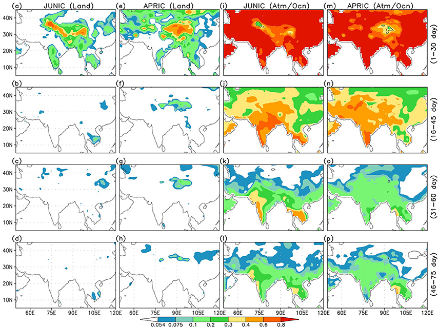
Figure 10. Potential predictability of 2 m air temperature in CFSv2 JUNIC hindcasts due to land initial conditions, expressed as a signal-to-total variance ratio and based on (a) 1–30 day, (b) 16–45 day, (c) 31–60 day and (d) 46–75 day averages. (e–h) respectively, show the same for APRIC hindcasts. (i–p) depict the potential predictability due to ocean initial conditions in JUNIC and APRIC hindcasts. All shaded areas are significant at the 95% confidence level. Black contours depict the areas where the variance ratios of signals due to land vs. ocean ICs are significant.

Deterministic Prediction Skill

Do we notice any discernible impact of realistic land ICs on the deterministic hindcast skill of 2 m air temperature? What role does land-atmosphere coupling play in enhancing the skill? To find answers to these questions we analyze the median anomaly correlation of CFSv2 JUNIC 2 m temperature hindcasts with CRU based on 27 RandLIC cases for the period 1982–2009 (Figure 11a), and based on those correlations assess the rank of the correlation for the hindcast based on RealLIC (Figure 11b). Correlations with IMD data are based on a shorter period (1982–2005). Enhancement in skill, depicted by an increase in the anomaly correlations and hence their rank, due to realistic land ICs is expected particularly over those regions where the LA coupling is strong. We compare the correlations for the first month when the impact of realistic land ICs is expected the most as well as the season (JJAS). Note that correlation values with CRU data greater (less) than 0.37 (−0.37) are significant. For IMD data, the corresponding values are ± 0.4. Significant skill in 2 m air temperature verified in June over the Indian region due to RandLICs may arise due to correct atmosphere and ocean ICs. For the season as a whole (JJAS), skill due to RandLICs is mostly confined to the east of CI, peninsular India and a small region to its west (Figure 11e). These spatial patterns in skill are mostly expected because of the proximity of those regions to the ocean (cf. Koster and Suarez, 1995).

FIGURE 11

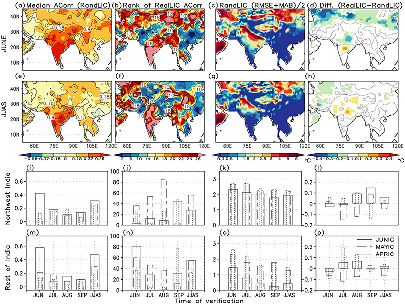
Figure 11. (a) median anomaly correlation of 2 m air temperature in June based on CFSv2 JUNIC hindcasts with RandLIC and CRU (shaded) and IMD (black contours). (b) rank of the anomaly correlation based on JUNIC hindcast with RealLIC among 28 ensemble members. (c) average of RMSE and MAB based on JUNIC hindcasts with RandLIC. (d) shows the difference of mean RMSE and MAB (RealLIC-RandLIC). (e–h) depict the same as in first row except for JJAS. (i,k,l,m,o,p) show the same for APRIC, MAYIC, and JUNIC hindcasts; except for each month in JJAS and area averaged for the northwest and rest of India domains, respectively. (j,n) depict the percentage area that shows RealLIC anomaly correlations in the upper quartile of the 28 ensemble members.

Based on the higher rank of the anomaly correlation obtained using RealLICs, one can conclude that the monthly forecast skill is enhanced in June mostly to the east of CI and peninsular India, but reduced over the northwest region, northern India, and the Himalayas (Figure 11b). As for the season (JJAS), there is also an increase in skill over the peninsula, CI and the north, but decrease over the northwest (Figure 11f). Areas showing an increase in skill indeed coincide with those regions where the LA coupling in the model is strong (cf. Figures 4, 8, 9). We shall further discuss the factors underlying those changes in the next section. Interestingly, there is also much enhancement in skill over the northeastern states of India, Myanmar, and parts of southeast Asia. A comparison using the two verification datasets helps in making a better objective assessment of the improvement in skill.

On monthly time scale, median skill due to RandLICs is the highest only during the first month and decreases thereafter in the season, for all start dates (Figures 11i,m). There is also a systematic increase in seasonal forecast skill of 2 m temperature with reduction in the forecast lead-time from April to June that indicates a dynamical drift in the model climatology. Interesting changes are noted when RealLICs are used for initialization. Over the rest of India domain highest increase in skill is shown by JUNIC hindcasts for June, followed by MAYIC and APRIC (Figure 11n). Contrary to that MAYIC hindcasts depict skill enhancement for July, August and JJAS over the northwest; unlike APRIC or JUNIC (Figure 11j). Such a feature has been reported in earlier studies as well (cf. Pokhrel et al., 2015) mentioning that May IC hindcasts have the highest skill in CFSv2 freeruns for JJAS that is mostly associated with slowly varying oceanic boundary conditions. On the other hand, APRIC and JUNIC hindcasts show an increase in skill due to RealLICs toward the end of the season (i.e., September).

As the spatial patterns of RMSE and MAB are similar, we have considered their average for an assessment. Large errors in simulated temperature in June and JJAS are noted over the Gangetic plains over northern India, near the Himalayan foothills, northwestern regions, and parts of CI due to RandLIC (Figures 11c,g). This implies that apart from the mean surface temperature bias (cf. Figure 3) the model is unable to accurately capture variability in surface temperature over those regions that also include areas having steep vertical gradient. Use of RealLIC is found to largely decrease those errors in June (Figure 11d); for JJAS only a few small areas tend to show an increase (Figure 11h). Monthly RMSE and MAB also systematically decrease over India for RandLICs, from April through June (Figures 11k,o). For RealLIC, the errors of JUNIC hindcasts are lower than that of APRIC (Figures 11l,p). However, they are lowest for MAYIC hindcasts.

Apart from temperature, there is enhancement in the precipitation forecast skill over India due to realistic land surface initialization, particularly over CI and the northwest region (not shown). However, the improvement that takes place only over few areas won't qualify for the field significance test. Furthermore, we also verify increased skill in precipitation over the northwest region in September (not shown) that might be associated with better simulation of the withdrawal of the monsoon.

Discussion

Plausible Mechanisms

Memory of the surface soil layer is short. However, soil moisture memory in the root zone can extend upto a month or two over certain regions and even upto a season for the layers further deep. The Indian summer monsoon is punctuated by alternating episodes of above and below normal rainfall activity on the intraseasonal time scale, and such fluctuations have dominant periodicities of 10–20 and 30–60 days (Goswami and Xavier, 2005). Therefore, during the course of the monsoon season under certain atmospheric conditions such as prolonged dry spells or drought when the land surface shifts to a drier regime, deeper layer soil moisture anomalies may strongly affect surface fluxes, near surface atmospheric variables and lower-tropospheric stability through transpiration and vertical movement of water in soil (cf. Saha et al., 2012). We propose that longer soil moisture memory in the root-zone and deeper layers is one of the prime reasons for changes in temperature (and precipitation) skill on sub-seasonal and seasonal time scales. To justify that, we demonstrate the median skill in rootzone soil moisture from JUNIC hindcasts (Figure 12). For verification, the global offline soil moisture analysis from GLDAS2 is used.

FIGURE 12

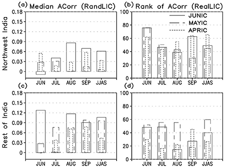
Figure 12. (a) median anomaly correlation of root zone soil moisture based on CFSv2 JUNIC, MAYIC and APRIC hindcasts with RandLIC and GLDAS2, in each month and JJAS, averaged over the northwest of India. (c) shows the same for the rest of India region. (b,d) depict the percentage area that shows RealLIC anomaly correlations in the upper quartile of the 28 ensemble members, for each month and JJAS, for the northwest and rest of Indian domains, respectively.

Unlike temperature, median anomaly correlation in root zone soil moisture due to RandLICs is low in all the months (Figures 12a,c). This is revealed from the area averaged values of the correlation over both regions. Much of the skill in soil moisture is derived from the skill in simulated precipitation due to RandLICs. When initialized with realisitc land states, large areas depict a significant increase in soil moisture skill not only over India but the entire south Asian region (not shown). Over the NWI (top right panel), there is increased soil moisture skill in June due to usage of realistic initial land surface states for all three initial start dates (Figure 12b). However, that does not appear to translate into skill of air temperature because of weak LA coupling over that region. Maximum enhancement in surface temperature skill in JUNIC and APRIC hindcasts with RealLICs, that could be attributed to the skill in simulated soil moisture is noted in September. It could also be that the withdrawal of the monsoon from the north and northwest regions of India in September is better captured in those simulations (not shown) that results in increased skill of soil moisture. Furthermore, part of the enhanced air temperature skill in July, August and JJAS in MAYIC runs could also be explained by the increased soil moisture skill in those months. On the other hand for the ROI, soil moisture skill due to realistic land surface initialization in June and May translates into air temperature skill only in June and JJAS (Figure 12d). For APRIC, that happens only in September.

There could be several factors contributing to the enhanced skill in surface temperature over India on sub-seasonal to seasonal time scales, such as the ocean (Pokhrel et al., 2015), snowmelt and associated hydrological effect over Eastern Eurasia (Halder and Dirmeyer, 2017) or land-use land-cover changes (Halder et al., 2016) that needs further investigation. Here, we explore the LA coupling pathway that links skill in local soil moisture anomalies to that of temperature and precipitation. Increased precipitation leads to an increase in ground wetness through infiltration, both at the surface and sub-surface. For vegetated surfaces, precipitation tends to have a high correlation with the evaporation of canopy intercepted water (CEVAP; not shown), especially in second generation land surface models such as the Noah where all leaves are assumed to be oriented parallel to the ground. Transpiration is completely shut-off when leaves are covered with water, leading to a strong negative correlation with CEVAP. This is mostly noted (for MAYIC runs) over western and CI, the WGs, east and northeast India and the foothills of the Himalayas (Figures 13a,e,i,m). While the negative correlations intensify with increasing precipitation over India from June through September, parts of northern and NWI and the rain-shadow region of eastern peninsular India that remain relatively drier show the opposite. On the other hand, bare ground evaporation (GEVAP) that is strongly controlled by surface soil moisture variability in arid to semi-humid regions may continue to be high. Root zone (and deeper layer) soil moisture can have a strong impact on surface moisture fluxes through transpiration (TRANSP) or vertical soil water movement, over areas where canopy evaporation has not completely shut it off. Figures 13b,f,j,n show that such anomalies can strongly control transpiration (and hence LHF) in those regions, as evidenced by the significant positive correlations during all the months. Negative correlations over the east and south of CI do not become significantly strong until in August. Therefore, it is verified that skill in root zone soil moisture anomalies can increase the skill of near surface variables such as temperature on sub-seasonal time scales. Such association is strongly reflected in the monthly TCI plots for RSW and TRANSP (Figures 13c,g,k,o) and RSW and GEVAP (Figures 13d,h,l,p). Over parts of CI in June and July where the correlations in surface transpiration are weakly negative, ground evaporation controlled by root zone soil wetness can also act to increase the skill of surface temperature through the modulation of the fluxes.

FIGURE 13

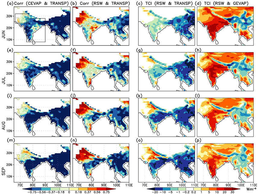
Figure 13. Corelation of transpiration (TRANSP) with (a) canopy evaporation (CEVAP,) and (b) root zone soil wetness (RSW) in June based on CFSv2 MAYIC hindcasts. Terrestrial coupling index (TCI) between RSW and (c) TRANSP and (d) ground evaporation (GEVAP) in June. Units for TCI are Wm⁻². (e–p) depict similar relationships for the months July, August, and September, respectively.

Summary

Land-atmosphere coupling is defined as the feedback link from land surface states to surface fluxes to atmospheric states and characteristics. The modern paradigm of land-atmosphere coupling proposes three ingredients must exist over a region for land surface states to translate into meaningful reponses in the atmosphere. The ingredients are sensitivity of downstream states/fluxes to variations in upstream states/fluxes, variability of upstream states/fluxes, and persistence of soil moisture anomalies at the first link in the chain. We investigate the impact of initial land states and land-atmosphere coupling on the predictability and prediction skill of Indian summer monsoon (June through September) rainfall and temperature through a suite of retrospective forecasts using the CFSv2 global coupled model. A large matrix of 28 × 28 hindcasts during 1982–2009 are used to demonstrate such impact.

Potential predictability in the model for near surface air temperature over India attributed to land ICs exists only in the first month and decreases thereafter. For other regions, such as extratropical vegetated or snow covered areas, there is discernible predictability at least for a few months during boreal summer and the preceeding spring. While predictability in precipitation for this model attributed to land ICs it is too weak to be significant, there is significant potential predictability associated with ocean-atmosphere ICs. Previous studies that demonstrate a weak correspondence between intial land states and subsequent precipitation anomalies over the Indian region (cf. Dirmeyer, 2013; Dirmeyer and Halder, 2017) also support our inference. There is however, significant deterministic skill improvement in the interannual anomalies of monthly and seasonal (JJAS) near surface temperatures due to realistic land surface initialization.

In general, all the hindcasts when realistically initialized at the land surface in June, May, or April show increased skill in monthly air temperature anomalies over the Indian region, except the northwest and north. Over northwest India, maximum skill improvement is noted in June and JJAS for hindcasts initialized in May; whereas highest skill improvement toward the end of the season is noted for April and June IC hindcasts. Improvements in skill due to realistic land surface initialization mostly take place over those areas where the land-atmosphere coupling is strong in the CFSv2 model. However, shortcomings in the accurate representation of coupling across the land-atmosphere interface due to systematic errors in the model prevent further improvement in the skill. It may be noted that while reanalysis based land surface fluxes depend on the quality of the model physics and the initial analysis and are known to have uncertainties; efforts are increasingly being made to reduce them, particularly in the moisture fluxes, by rectifying errors in the simulated precipitation forcing using observational constraints and allowing the land surface model physics to respond (cf. Meng et al., 2012; Draper et al., 2017). There could also be large-scale factors other than local land-atmosphere coupling that contribute toward improved sub-seasonal to seasonal air temperature skill due to May ICs. Although, there are improvements in the prediction skill of precipitation due to realistic land surface initialization, changes over India are confined over relatively lesser areas. Innovative design of experiments and an improved atmospheric model would be needed to better demonstrate such skill enhancement.

There is skill in simulated soil moisture at the surface and sub-surface layers that contributes toward an improvement in temperature skill on monthly (sub-seasonal) and seasonal time scales, through changes in transpiration and ground evaporation fluxes. However, due to the lack of a dense network of rain-gauge observations in the areas further to the northwest of India, the uncertainty associated with soil moisture values has also to be accounted for. It is proposed that long soil moisture memory within the deeper soil layers can help in the persistence of realistic initial land states and lead to the reemergence or improvement in skill of near surface air temperature over certain regions, provided the necessary ingredients of strong land-atmosphere coupling are present. Such mechanisms shall be explored in a follow-up study.

We speculate that better simulation of the timing of withdrawal of the monsoon from the northwest of India could also be a cause of increased skill in precipitation and surface air temperature (not shown), at the end of the monsoon season. There could also be other complex processes at the soil-vegetation-atmosphere interface, such as land-use land-cover change and associated changes in surface albedo, moisture and radiation fluxes that leads to changes in skill on sub-seasonal or extended range time scale. However, such detailed investigation of plausible causes shall be made in future endeavours. Nevertheless, several factors already discussed the section Restuls that could lead to the minimization of the predictability from initial land states and degradation of forecast skill stand out in this study. They include errors in the parameterization of radiation, shallow and deep cumulus convection; a boundary layer scheme that poorly represents vertical eddy diffusivity; surface moisture fluxes and representation of vegetation. Apart from that, incorrect representation of daily and sub-daily precipitation statistics arising from errors in the diurnal cycle of convection over land in CFSv2 are also likely responsible for errors in land-atmosphere coupling. There could be further improvement in the skill of Indian sumer monsoon simulations if accurate initial land states and a network of in-situ surface flux (micrometeorological) observations for the verification of land-atmosphere coupling were available. Therefore, for improved simulation of the Indian summer monsoon on different time scales, a concerted effort is needed for improvement of the land-ocean-atmosphere coupled processes in weather and climate models.

Author Contributions

SH and PD conceptualized and designed the present work. LM provided significant contributions in completion of the model experiments. PD and JK provided valuable inputs in interpretation of the data. SH wrote the manuscript with inputs from PD. Further, all co-authors revised the manuscript and gave consent to its final form.

Funding

We acknowledge support from the National Monsoon Mission, Ministry of Earth Sciences, Government of India. We also acknowledge support from NSF (AGS-1338427), NOAA (NA14OAR4310160) and NASA (NNX14AM19G).

Conflict of Interest Statement

The authors declare that the research was conducted in the absence of any commercial or financial relationships that could be construed as a potential conflict of interest.

Acknowledgments

We thank the National Monsoon Mission, Ministry of Earth Sciences, Government of India for support to carry out this study. GLDAS-2.0 data is obtained from http://disc.sci.gsfc.nasa.gov/hydrology/data-holdings. Data from the SRBE are obtained from the NASA Langley Research Center Atmospheric Sciences Data Center NASA/GEWEX SRB Project. We also acknowledge the Texas Advanced Computing Center (TACC) at The University of Texas at Austin for providing high performance computing resources. Data from all the model simulations reside on the TACC Ranch advanced storage resource.

Supplementary Material

The Supplementary Material for this article can be found online at: https://www.frontiersin.org/articles/10.3389/fenvs.2017.00092/full#supplementary-material

References

Adler, R. F., Huffman, G. J., Chang, A., Ferraro, R., Xie, P., Janowiak, J., et al. (2003). The version-2 Global Precipitation Climatology Project (GPCP) monthly precipitation analysis (1979–Present). J. Hydrometeorol. 4, 1147–1167. doi: 10.1175/1525-7541(2003)004<1147:TVGPCP>2.0.CO;2

CrossRef Full Text | Google Scholar

Ashfaq, M., Rastogi, D., Mei, R., Touma, D., and Leung, R. (2017). Sources of errors in the simulation of south Asian summer monsoon in the CMIP5 GCMs. Clim. Dyn. 49, 193–223. doi: 10.1007/s00382-016-3337-7

CrossRef Full Text | Google Scholar

Barker, H. W., Pincus, R., and Morcrette, J. J. (2002). “The Monte Carlo independent column approximation: application within large-scale models,” in Extended Abstracts, GCSS-ARM Workshop on the Representation of Cloud Systems in Large-Scale Models (Kananaskis, AB: GEWEX), 1–10.

Bollasina, M. A., and Ming, Y. (2013). The role of land surface processes in modulating the Indian monsoon annual cycle. Clim. Dyn. 41, 2497–2509. doi: 10.1007/s00382-012-1634-3

CrossRef Full Text | Google Scholar

Bombardi, R. J., Schneider, E. K., Marx, L., Halder, S., Singh, B., Tawfik, A. B., et al. (2015). Improvements in the representation of the Indian Summer Monsoon in the NCEP Climate Forecast System version 2. Clim. Dyn. 45, 2485–2498. doi: 10.1007/s00382-015-2484-6

CrossRef Full Text | Google Scholar

Cavalieri, D. J., Parkinson, C., Gloersen, P., and Zwally, H. J. (2007). Sea Ice Concentrations from Nimbus-7 SMMR and DMSP SSM/I Passive Microwave Data, 1978-1996. Boulder, CO: National Snow and Ice Data Center, Digital Media.

Cavalieri, D., Parkinson, C., Gloersen, P., and Zwally, H. J. (1996). Sea Ice Concentrations from Nimbus-7 SMMR and DMSP SSM/I-SSMIS Passive Microwave Data, Version 1. Boulder, CO: NASA DAAC at the National Snow and Ice Data Center.

Charney, J., Stone, P. H., and Quirk, W. J. (1975). Drought in the Sahara: a biogeophysical feedback mechanism. Science 187, 434–435. doi: 10.1126/science.187.4175.434

PubMed Abstract | CrossRef Full Text

Chen, M., Shi, W., Xie, P., Silvs, V. B. S., Kousky, V. E., Higgins, R. W., et al. (2008). Assessing objective techniques for gauge-based analyses of global daily precipitation. J. Geophys. Res. 113:D04110. doi: 10.1029/2007JD009132

CrossRef Full Text | Google Scholar

Clough, S. A., Shephard, M. W., Mlawer, E. J., Delamere, J. S., Iacono, M. J., Cady-Pereira, K., et al. (2005). Atmospheric radiative transfer modeling: a summary of the AER codes. J. Quant. Spectrosc. Radiat. Transfer 91, 233–244. doi: 10.1016/j.jqsrt.2004.05.058

CrossRef Full Text | Google Scholar

DelSole, T., and Shukla, J. (2012). Climate models produce skillful predictions of Indian summer monsoon rainfall. Geophys. Res. Lett. 39:9. doi: 10.1029/2012GL051279

CrossRef Full Text | Google Scholar

Dirmeyer, P. A. (2003). The role of the land surface background state in climate predictability. J. Hydrometeor. 4, 599–610. doi: 10.1175/1525-7541(2003)004<0599:TROTLS>2.0.CO;2

CrossRef Full Text | Google Scholar

Dirmeyer, P. A. (2005). The land surface contribution to boreal summer season predictability. J. Hydrometeor. 6, 618–632. doi: 10.1175/JHM444.1

CrossRef Full Text

Dirmeyer, P. A. (2006). The hydrologic feedback pathway for land-climate coupling. J. Hydrometeor. 7, 857–867. doi: 10.1175/JHM526.1

CrossRef Full Text | Google Scholar

Dirmeyer, P. A. (2011). The terrestrial segment of soil moisture–climate coupling. Geophys. Res. Lett. 38:L16702. doi: 10.1029/2011GL048268

CrossRef Full Text | Google Scholar

Dirmeyer, P. A. (2013). Characteristics of the water cycle and land-atmosphere interactions from a comprehensive reforecast and reanalysis data set: CFSv2. Clim. Dyn. 41, 1083–1097. doi: 10.1007/s00382-013-1866-x

CrossRef Full Text | Google Scholar

Dirmeyer, P. A., Wang, Z., Mbuh, M. J., and Norton, H. E. (2014). Intensified land surface control on boundary layer growth in a changing climate. Geophys. Res. Lett. 41, 1290–1294. doi: 10.1002/2013GL058826

CrossRef Full Text | Google Scholar

Dirmeyer, P. A., Wu, J., Norton, H. E., Dorigo, W. A., Quiring, S. M., Ford, T. M., et al. (2016). Confronting weather and climate models with observational data from soil moisture networks over the United States. J. Hydrometeor. 17, 1049–1067. doi: 10.1175/JHM-D-15-0196.1

CrossRef Full Text | Google Scholar

Dirmeyer, P. A., and Halder, S. (2016). Sensitivity of numerical weather forecasts to initial soil moisture variations in CFSv2. Wea. Forecast. 31, 1973–1983. doi: 10.1175/WAF-D-16-0049.1

CrossRef Full Text | Google Scholar

Dirmeyer, P. A., and Halder, S. (2017). Application of the land-atmosphere coupling paradigm to the operational Coupled Forecast System (CFSv2) model. J. Hydrometeorol. 18, 85–108. doi: 10.1175/JHM-D-16-0064.1

CrossRef Full Text | Google Scholar

Dirmeyer, P. A., Schlosser, C. A., and Brubaker, K. L. (2009). Precipitation, recycling and land memory: an integrated analysis. J. Hydrometeor. 10, 278–288. doi: 10.1175/2008JHM1016.1

CrossRef Full Text | Google Scholar

Draper, C., Reichle, R. H., and Koster, R. (2017). Assessment of MERRA-2 land surface energy flux estimates. J. Clim. doi: 10.1175/JCLI-D-17-0121.1. [Epub ahead of print].

CrossRef Full Text | Google Scholar

Ek, M. B., Mitchell, K. E., Lin, Y., Rogers, E., Grunmann, P., Koren, V., et al. (2003). Implementation of Noah land surface model advances in the National Centers for Environmental Prediction operational mesoscale Eta model. J. Geophys. Res. 108:8851. doi: 10.1029/2002JD003296

CrossRef Full Text | Google Scholar

Ferranti, L., Slingo, J., Palmer, T. N., and Hoskins, B. J. (1999). The effect of land-surface feedbacks on the monsoon circulation. Q. J. R. Meteorol. Soc. 125, 1527–1550. doi: 10.1002/qj.49712555704

CrossRef Full Text | Google Scholar

Findell, K. L., and Eltahir, E. A. B. (2003a). Atmospheric controls on soil moisture-boundary layer interactions: Part I: framework development. J. Hydrometeor. 4, 552–569. doi: 10.1175/1525-7541(2003)004<0552:ACOSML>2.0.CO;2

CrossRef Full Text | Google Scholar

Findell, K. L., and Eltahir, E. A. B. (2003b). Atmospheric controls on soil moisture– boundary layer interactions. Part II: feedbacks within the continental United States. J. Hydrometeor. 4, 570–583. doi: 10.1175/1525-7541(2003)004<0570:ACOSML>2.0.CO;2

CrossRef Full Text | Google Scholar

Gadgil, S., Vinayachandran, P. N., and Francis, P. A. (2003). Droughts of the Indian summer monsoon: role of clouds over the Indian Ocean. Curr. Sci. 85, 1713–1719.

Google Scholar

Gelaro, R., McCarty, W., Suarez, M. J., Todling, R., Molod, A., Takacs, L., et al. (2017). The modern-era retrospective analysis for research and applications, Version 2 (MERRA-2). J. Clim. 30, 5419–5454. doi: 10.1175/JCLI-D-16-0758.1

CrossRef Full Text | Google Scholar

Goswami, B. N., and Chakravorty, S. (2017). “Dynamics of the Indian summer monsoon climate,” in Oxford Research Encyclopedia of Climate Science, ed H. Von Storch (Oxford University Press), 38.

Goswami, B. N., Madhusoodanan, M. S., Neema, C. P., and Sengupta, D. (2006). A physical mechanism for North Atlantic SST influence on the Indian summer monsoon. Geophys. Res. Lett. 33:L02706. doi: 10.1029/2005GL024803

CrossRef Full Text | Google Scholar

Goswami, B. N., and Xavier, P. K. (2005). Dynamics of “internal” interannual variability of the Indian summer monsoon in a GCM. J. Geophys. Res. Atmos. 110:D24104. doi: 10.1029/2005JD006042

CrossRef Full Text | Google Scholar

Goswami, T., Rao, S. A., Hazra, A., Chaudhari, H. S., Dhakate, A., Salunke, K., et al. (2017). Assessment of simulation of radiation in NCEP Climate Forecast System (CFS v2). Atmos. Res. 193, 94–106. doi: 10.1016/j.atmosres.2017.04.013

CrossRef Full Text | Google Scholar

Griffies, S. M., Harrison, M. J., Pacanowski, R. C., and Rosati, A. (2004). A Technical Guide to MOM4. GFDL Ocean Group Technical Report no. 5, 281. Available online at: http://data1.gfdl.noaa.gov/~arl/pubrel/j/mom4beta/src/mom4/doc/guide.pdf

Grumbine, R. W. (1996). Automated Passive Microwave Sea Ice Concentration Analysis at NCEP. NCEP OMB Tech. Note 120, 13.

Guo, Z., Dirmeyer, P. A., and DelSole, T. (2011). Land surface impacts on subseasonal and seasonal predictability. Geophys. Res. Lett. 38:L24812. doi: 10.1029/2011GL049945

CrossRef Full Text | Google Scholar

Guo, Z., Dirmeyer, P. A., DelSole, T., and Koster, R. D. (2012). Rebound in atmospheric predictability and the role of the land surface. J. Clim. 25, 4744–4749. doi: 10.1175/JCLI-D-11-00651.1

CrossRef Full Text | Google Scholar

Guo, Z., Dirmeyer, P. A., Koster, R. D., Sud, Y. C., Bonan, C., Oleson, K. W., et al. (2006). GLACE: the global land–atmosphere coupling experiment. Part II: analysis. J. Hydrometeor. 7, 611–625. doi: 10.1175/JHM511.1

CrossRef Full Text | Google Scholar

Halder, S., and Dirmeyer, P. A. (2017). Relation of Eurasian snow cover and Indian summer monsoon rainfall: importance of the delayed hydrological effect. Am. Meteorol. Soc. 30, 1273–1289. doi: 10.1175/JCLI-D-16-0033.1

CrossRef Full Text | Google Scholar

Halder, S., Dirmeyer, P. A., and Saha, S. K. (2015). Sensitivity of the mean and variability of Indian summer monsoon to land surface schemes in RegCM4: understanding coupled land-atmosphere feedbacks. J. Geophys. Res. 120, 9437–9458. doi: 10.1002/2015JD023101

CrossRef Full Text | Google Scholar

Halder, S., Saha, S. K., Dirmeyer, P. A., Chase, T. N., and Goswami, B. N. (2016). Investigating the impact of land-use land-cover change on Indian summer monsoon daily rainfall and temperature during 1951-2005 using a regional climate model. Hydrol. Earth Syst. Sci. 20, 1765–1784. doi: 10.5194/hess-20-1765-2016

CrossRef Full Text | Google Scholar

Harris, I., Jones, P. D., Osborn, T. J., and Lister, D. H. (2014). Updated high-resolution grids of monthly climatic observations - the CRU TS3.10 Dataset. Int. J. Climatol. 34, 623–642. doi: 10.1002/joc.3711

CrossRef Full Text | Google Scholar

Hirsch, A., Pitman, A. J., and Haverd, V. (2016). Evaluating land-atmosphere coupling using a resistance pathway framework. J. Hydrometeorol. 17, 2615–2630. doi: 10.1175/JHM-D-15-0204.1

CrossRef Full Text | Google Scholar

Hong, S. Y., and Pan, H. L. (1996). Nonlocal boundary layer vertical diffusion in a medium-range forecast model. Mon. Wea. Rev. 124, 2322–2339.

Google Scholar

Kim, H. M., Webster, P. J., Curry, J. A., and Toma, V. E. (2012). Asian summer monsoon prediction in ECMWF System 4 and NCEP CFSv2 retrospective seasonal forecasts. Clim. Dyn. 39, 2975–2299. doi: 10.1007/s00382-012-1470-5

CrossRef Full Text | Google Scholar

Koster, R. D., Dirmeyer, P. A., Guo, Z., Bonan, G., Chan, E., Cox, P., et al. (2004). Regions of strong coupling between soil moisture and precipitation. Science 305, 1138–1140. doi: 10.1126/science.1100217

PubMed Abstract | CrossRef Full Text | Google Scholar

Koster, R. D., Mahanama, S. P. P., Yamada, T. J., Balsamo, G., Berg, A. A., Boisserie, M., et al. (2010). Contribution of land surface initialization to subseasonal forecast skill: first results from a multi-model experiment. Geophys. Res. Lett. 37:L02402. doi: 10.1029/2009GL041677

CrossRef Full Text | Google Scholar

Koster, R. D., Mahanama, S. P. P., Yamada, T. J., and Wood, E. F. (2011). The second phase of the Global Land-Atmosphere Coupling Experiment: soil moisture contributions to subseasonal forecast skill. J. Hydrometeor. 12, 805–822. doi: 10.1175/2011JHM1365.1

CrossRef Full Text | Google Scholar

Koster, R. D., and Suarez, M. J. (1995). Relative contributions of land and ocean processes to precipitation variability. J. Geophys. Res. 100, 13775–13790. doi: 10.1029/95JD00176

CrossRef Full Text | Google Scholar

Koster, R. D., and Suarez, M. J. (2004). Suggestions in the observational record of land-atmosphere feedback operating at seasonal timescales. J. Hydrometeor. 5, 567–572.

Google Scholar

Kumar, K., Hoerling, M., and Rajagopalan, B. (2005). Advancing dynamical prediction of Indian monsoon rainfall. Geophys. Res. Lett. 32:L08704. doi: 10.1029/2004GL021979

CrossRef Full Text | Google Scholar

Kumar, K., Rajagopalan, B., Hoerling, M., Bates, G., and Cane, M. (2006). Unraveling the mystery of Indian monsoon failure during El Nino. Science 3146, 115–119. doi: 10.1126/science.1131152

CrossRef Full Text | Google Scholar

Lorenz, R., Pitman, A. J., Hirsch, A. L., and Srbinovsky, J. (2016). Intraseasonal versus interannual measures of land–atmosphere coupling strength in a global climate model: GLACE-1 versus GLACE-CMIP5 experiments in ACCESS1. 3b. J. Hydrometeorol. 16, 2276–2295. doi: 10.1175/JHM-D-14-0206.1

CrossRef Full Text

Meng, J., Yang, R., Wei, H., Ek, M., Gayno, G., Xie, P., et al. (2012). The land surface analysis in the NCEP Climate Forecast System Reanalysis. J. Hydrometeorol. 13, 1621–1630. doi: 10.1175/JHM-D-11-090.1

CrossRef Full Text | Google Scholar

Mlawer, E. J., Taubman, S. J., Brown, P. D., Iacono, M. J., and Clough, S. A. (1997). Radiative transfer for inhomogeneous atmosphere: RRTM, a validated correlated-k model for the longwave. J. Geophys. Res. 102, 16663–16682. doi: 10.1029/97JD00237

CrossRef Full Text | Google Scholar

Nanjundiah, R. S., Francis, P. A., Ved, M., and Gadgil, S. (2013). Predicting the extremes of Indian summer monsoon rainfall with coupled ocean-atmosphere models. Curr. Sci. 104, 1380–1393.

Google Scholar

Pincus, R., Barker, H. W., and Morcrette, J. J. (2003). A fast, flexible, approximate technique for computing radiative transfer in inhomogeneous cloud fields. J. Geophys. Res. 108:4376. doi: 10.1029/2002JD003322

CrossRef Full Text | Google Scholar

Pokhrel, S., Saha, S. K., Dhakate, A., Rahman, H., Chaudhari, H. S., Salunke, K., et al. (2015). Seasonal prediction of Indian summer monsoon rainfall in NCEP CFSv2: forecast and predictability error. Clim. Dyn. 46, 2305–2326. doi: 10.1007/s00382-015-2703-1

CrossRef Full Text | Google Scholar

Rai, S., and Krishnamurthy, V. (2011). Error growth in climate forecast system daily retrospective forecasts of South Asian monsoon. J. Geophys. Res. 116:D03108. doi: 10.1029/2010JD014840

CrossRef Full Text | Google Scholar

Rajeevan, M., Unnikrishnan, C. K., and Preethi, B. (2012). Evaluation of the ENSEMBLES multi-model seasonal forecasts of Indian summer monsoon variability. Clim. Dyn. 38, 2257–2274. doi: 10.1007/s00382-011-1061-x

CrossRef Full Text | Google Scholar

Ramu, D. A., Sabeerali, C. T., Chattopadhyay, R., Rao, D. N., George, G., Dhakate, A. R., et al. (2016). Indian summer monsoon rainfall simulation and prediction skill in the CFSv2 coupled model: impact of atmospheric horizontal resolution. J. Geophys. Res. Atmos 121, 2205–2221. doi: 10.1002/2015JD024629

CrossRef Full Text | Google Scholar

Reynolds, R. W., Smith, T. M., Liu, C., Chelton, D. B., Casey, K. S., and Schlax, M. G. (2007). Daily high-resolution blended analyses for sea surface temperature. J. Clim. 20, 5473–5496. doi: 10.1175/2007JCLI1824.1

CrossRef Full Text | Google Scholar

Rodell, M., Houser, R. P., Jambor, U., Gottschalck, J., Mitchell, K., Meng, C.-J., et al. (2004). The global land data assimilation system. Bull. Amer. Meteor. Soc. 85, 381–394. doi: 10.1175/BAMS-85-3-381

CrossRef Full Text | Google Scholar

Saha, S., Moorthi, S., Pan, H. L., Wu, X., Wang, J., Nadiga, S., et al. (2010). The NCEP climate forecast system reanalysis. Bull. Amer. Meteor. Soc. 91, 1015–1057. doi: 10.1175/2010BAMS3001.1

CrossRef Full Text | Google Scholar

Saha, S., Moorthi, S., Wu, X., Wang, J., Nadiga, S., Tripp, P., et al. (2014). The NCEP climate forecast system version 2. J. Clim. 27, 2185–2208. doi: 10.1175/JCLI-D-12-00823.1

CrossRef Full Text | Google Scholar

Saha, S. K., Halder, S., Kumar, K. K., and Goswami, B. N. (2011). Pre-onset land surface processes and internal interannual variabilities of the Indian summer monsoon. Clim. Dyn. 36, 2077–2089. doi: 10.1007/s00382-010-0886-z

CrossRef Full Text | Google Scholar

Saha, S. K., Halder, S., Rao, A. S., and Goswami, B. N. (2012). Modulation of ISOs by land-atmosphere feedback and contribution to the interannual variability of Indian Summer Monsoon. J. Geophys. Res. 117:D13101. doi: 10.1029/2011JD017291

CrossRef Full Text | Google Scholar

Saha, S. K., Sujith, K., Pokhrel, S., Chaudhari, H. S., and Hazra, A. (2017). Effects of multilayer snow scheme on the simulation of snow: offline Noah and coupled with NCEP CFSv2. J. Adv. Model. Earth Syst. 9, 271–290. doi: 10.1002/2016MS000845

CrossRef Full Text | Google Scholar

Sahai, A. K., Abhilash, S., Chattopadhyay, R., Borah, N., Joseph, S., Sharmila, S., et al. (2015). High-resolution operational monsoon forecasts: an objective assessment. Clim. Dyn. 44, 3129–3140. doi: 10.1007/s00382-014-2210-9

CrossRef Full Text | Google Scholar

Saji, N. H., Goswami, B. N., Vinaychandran, P. N., and Yamagata, T. (1999). A dipole mode in the tropical Indian Ocean. Nature 401, 360–363. doi: 10.1038/43854

PubMed Abstract | CrossRef Full Text | Google Scholar

Senan, R., Orsolini, Y. J., Weisheimer, A., Vitart, F., Balsamo, G., Stockdale, T. N., et al. (2016). Impact of springtime Himalayan-Tibetan Plateau snowpack on the onset of the Indian summer monsoon in coupled seasonal forecasts. Clim. Dyn. 47, 9–10, 2709–2725. doi: 10.1007/s00382-016-2993-y

CrossRef Full Text | Google Scholar

Shukla, J. (1985). Predictability. Adv. Geophys. 28B, 87–122. doi: 10.1016/S0065-2687(08)60186-7

CrossRef Full Text | Google Scholar

Shukla, J., Marx, L., Paolino, D., and Straus, D. (2000). Dynamical seasonal prediction. Bull. Amer. Meteor. Soc. 81, 2593–2606. doi: 10.1175/1520-0477(2000)081<2593:DSP>2.3.CO;2

CrossRef Full Text | Google Scholar

Shukla, J., and Mintz, Y. (1982). Influence of land-surface evapotranspiration on the earth's climate. Science 215, 1498–1501.

PubMed Abstract | Google Scholar

Sperber, K. R., Annamalai, H., Kang, I.-S., Kitoh, A., Moise, A., Turner, A., et al. (2013). The Asian summer monsoon: an intercomparison of CMIP5 vs. CMIP3 simulations of the late 20th century. Clim. Dyn. 41, 2711–2744. doi: 10.1007/s00382-012-1607-6

CrossRef Full Text | Google Scholar

Srivastava, A. K., Rajeevan, M., and Kshirsagar, S. R. (2009). Development of a highresolution daily gridded temperature data set (1969-2005) for the Indian region. Atmos. Sci. Lett. 10, 249–254. doi: 10.1002/asl.232

CrossRef Full Text | Google Scholar

Stackhouse, P. W., and Gupta, S. K. (2013). ISLSCP II Surface Radiation Budget (SRB) Radiation Data. Oak Ridge, TN: ORNL DAAC.

Tiedtke, M. (1983). “The sensitivity of the time-mean large-scale flow to cumulus convection in the ECMWF model,” in ECMWF Workshop on Convection in Large-Scale Models (Reading, ECMWF), 297–316.

Tiwari, S., Kar, S. C., and Bhatla, R. (2016). Examination of snowmelt over western Himalayas using remote sensing data. Theor. Appl. Climatol. 125, 227–239. doi: 10.1007/s00704-015-1506-y

CrossRef Full Text | Google Scholar

Turner, A. G., and Slingo, J. (2011). Using idealized snow forcing to test teleconnections with the Indian summer monsoon in the Hadley Centre GCM. Clim. Dyn. 36, 1717–1735. doi: 10.1007/s00382-010-0805-3

CrossRef Full Text | Google Scholar

Webster, P. J. (1983). Mechanisms of monsoon low-frequency variability: surface hydrological effects. J. Atmos. Sci. 40, 2110–2124.

Google Scholar

Wei, J., and Dirmeyer, P. A. (2010). Toward understanding the large-scale land-atmosphere coupling in the models: roles of different processes. Geophys. Res. Lett. 37:L19707. doi: 10.1029/2010GL044769

CrossRef Full Text | Google Scholar

Xie, P., and Arkin, P. A. (1997). Global precipitation: A 17- year monthly analysis based on gauge observations, satellite estimates, and numerical model outputs. Bull. Amer. Meteor. Soc. 78, 2539–2558.

Google Scholar

Xie, P., Chen, M., Yatagai, A., Hayasaka, T., Fukushima, Y., and Yang, S. (2007). A gauge-based analysis of daily precipitation over East Asia. J. Hydrometeor. 8, 607–626. doi: 10.1175/JHM583.1

CrossRef Full Text | Google Scholar

Yang, S., Wen, M., Yang, R., Higgins, W., and Zhang, R. (2011). Impacts of land process on the onset and evolution of Asian summer monsoon in the NCEP climate forecast system. Adv. Atmos. Sci. 28, 1301–1317. doi: 10.1007/s00376-011-0167-8

CrossRef Full Text | Google Scholar

Yasunari, T. (2007). Role of land-atmosphere interaction on Asian monsoon climate. J. Meteor. Soc. Jpn. 85B, 55–75. doi: 10.2151/jmsj.85B.55

CrossRef Full Text | Google Scholar

Zhang, L., Dirmeyer, P. A., Wei, J., Guo, Z., and Lu, C. H. (2011). Land-atmosphere coupling strength in the global forecast system. J. Hydrometeorol. 12, 147–156. doi: 10.1175/2010JHM1319.1

CrossRef Full Text | Google Scholar