Abstract
Determining how microbial communities organize and function at the ecosystem level is essential to understanding and predicting how they will respond to environmental change. Mathematical models can be used to describe these communities, but properly representing all the biological interactions in extremely diverse natural microbial ecosystems in a mathematical model is challenging. We examine a complementary approach based on the maximum entropy production (MEP) principle, which proposes that systems with many degrees of freedom will likely organize to maximize the rate of free energy dissipation. In this study, we develop an MEP model to describe biogeochemistry observed in Siders Pond, a phosphate limited meromictic system located in Falmouth, MA that exhibits steep chemical gradients due to density-driven stratification that supports anaerobic photosynthesis as well as microbial communities that catalyze redox cycles involving O, N, S, Fe, and Mn. The MEP model uses a metabolic network to represent microbial redox reactions, where biomass allocation and reaction rates are determined by solving an optimization problem that maximizes entropy production over time, and a 1D vertical profile constrained by an advection-dispersion-reaction model. We introduce a new approach for modeling phototrophy and explicitly represent oxygenic photoautotrophs, photoheterotrophs and anoxygenic photoautotrophs. The metabolic network also includes reactions for aerobic organoheterotrophic bacteria, sulfate reducing bacteria, sulfide oxidizing bacteria and aerobic and anaerobic grazers. Model results were compared to observations of biogeochemical constituents collected over a 24 h period at 8 depths at a single 15 m deep station in Siders Pond. Maximizing entropy production over long (3 day) intervals produced results more similar to field observations than short (0.25 day) interval optimizations, which support the importance of temporal strategies for maximizing entropy production over time. Furthermore, we found that entropy production must be maximized locally instead of globally where energy potentials are degraded quickly by abiotic processes, such as light absorption by water. This combination of field observations and modeling results indicate that natural microbial systems can be modeled by using the maximum entropy production principle applied over time and space using many fewer parameters than conventional models.
Introduction
Mass and energy flow associated with the growth and predation of bacteria, archaea and eukaryotes in microbial food webs, coupled with abiotic reactions and transport processes, define biogeochemical cycles that occur in ecosystems ranging in size from less than a liter (Marino et al., 2016) to the entire planet. Because organisms are ultimately responsible for most observed biogeochemical transformations, it is customary and natural to focus on the bioenergetics of growth and predation of organisms that constitute food webs in order to understand and predict biogeochemical transformations. This organismal focus has a long history and has advanced our understanding and prediction of ecosystem dynamics and the mass and energy flow through them (Riley, 1946; Fasham et al., 1990; Le Quere et al., 2005; Friedrichs et al., 2007; Schartau et al., 2017). While focusing on the growth, predator-prey and cooperative interactions of organisms will continue to contribute to our understanding of ecosystem bioenergetics, there are some challenges that limit this approach for microbial systems that form the basis of biogeochemical cycles. Microbial communities are diverse, complex and abundant, consisting, for example, of approximately 109 microorganisms per liter of seawater, with estimates that Earth hosts close to 1 trillion microbial species (Sogin et al., 2006; Locey and Lennon, 2016). With the advent of metagenomics, next generation sequencing and bioinformatics, the challenging task of deciphering and annotating the metabolic capabilities and activities of bacteria and other microorganisms has begun, but determining how information in genomes contributes to competition and cooperation is still in its infancy (Hallam and McCutcheon, 2015; Pasternak et al., 2015; Worden et al., 2015). Even more challenging is understanding and predicting community composition dynamics and succession as environmental conditions change, both from exogenous and endogenous drivers (Konopka et al., 2015). While considerable progress is being made in developing predictive models of biogeochemistry based on organisms and the genes they carry (Reed et al., 2014; Coles et al., 2017), the ability for this approach to encompass the complex biogeochemistry of the ecosystem will likely take many decades to compile and decipher. We believe the reductionist approach is essential, but there is also a complementary approach to understanding microbial biogeochemistry that is less studied and uses a more thermodynamic, or whole systems, approach.
Understanding how ecosystems function at the systems level has a long tradition in theoretical ecology (Chapman et al., 2016; Vallino and Algar, 2016), with the underlying premise that ecosystems organize so as to maximize an objective function, such as maximizing power proposed by Lotka (1922) nearly 100 years ago. The advantage of the systems approach is that optimization can be used to determine how an ecosystem will organize and function without the knowledge of which organisms are present and how their population changes over time. Understanding and modeling of ecosystems can focus on function rather than on organisms, and there is growing support that stable function arises from dynamic communities (Fernandez et al., 1999; Fernandez-Gonzalez et al., 2016; Louca and Doebeli, 2016; Needham and Fuhrman, 2016; Coles et al., 2017). Here, we build upon the assumption that microbial systems organize to use all available energy sources. To use the correct thermodynamic term, living organisms use Gibbs free energy, since energy is conserved, but Gibbs free energy (aka usable energy) is not. The destruction of Gibbs free energy or energy potentials results in entropy production, so the net action of life produces entropy, because contrary to conventional wisdom, living organisms are not low entropy structures (Morrison, 1964; Blumenfeld, 1981). This allows us to employ the maximum entropy production (MEP) principle, which proposes that systems with sufficient degrees of freedom will likely organize to maximize the dissipation of Gibbs free energy (Dewar, 2003; Lorenz, 2003; Martyushev and Seleznev, 2006). In an ecological context, if food (which includes organisms themselves) is available but not being consumed, then organisms will eventually adapt, invade or evolve to utilize it if biologically possible. This simple concept forms the basis of this manuscript. The MEP principle has been applied to both abiotic and biotic processes (Kleidon and Lorenz, 2005; Kleidon et al., 2010; Dewar et al., 2014b), and we have used MEP to model periodically forced methanotrophic microbial communities (Vallino et al., 2014) and investigate metabolic switching in nitrate reducing environments (Algar and Vallino, 2014). While MEP is consistent with Darwinian evolution, and likely guides its trajectory (Goldenfeld and Woese, 2011; Skene, 2015, 2017; Judson, 2017), it has yet to gain general acceptance in theoretical or experimental ecological communities largely because of an insufficient number of case studies and uncertainty in how to apply it.
In this study we develop an MEP-based model to predict microbial biogeochemistry in a meromictic pond located in Falmouth, MA (Siders Pond) that includes metabolic processes for phytoplankton, green sulfur bacteria, aerobic organoheterotrophic bacteria, sulfate reducing bacteria, sulfide oxidizing bacteria, photoheterotrophs and aerobic and anaerobic predators (Figure 1). However, the model's objective function is to dissipate energy potentials, not grow organisms. While previous MEP models have been developed for chemolithoautotrophs, chemolithoheterotrophs, and chemoorganoheterotrophs, this study expands the metabolic reaction repertoire to include photoautotrophs and photoheterotrophs. The approach is also extended to include an explicit spatial dimension, and we compare model output to observations in Siders Pond collected over a 24 h sampling period from eight depths. MEP solutions using two different optimization timescales (0.25 day vs. 3.0 days) are contrasted and compared to observations, and we discuss the problem of local vs. global MEP optimization for energy potentials that are quickly dissipated abiotically, such as light. Our results suggest that microbial systems in nature can be described by the maximum entropy production conjecture applied over time and space.
Figure 1
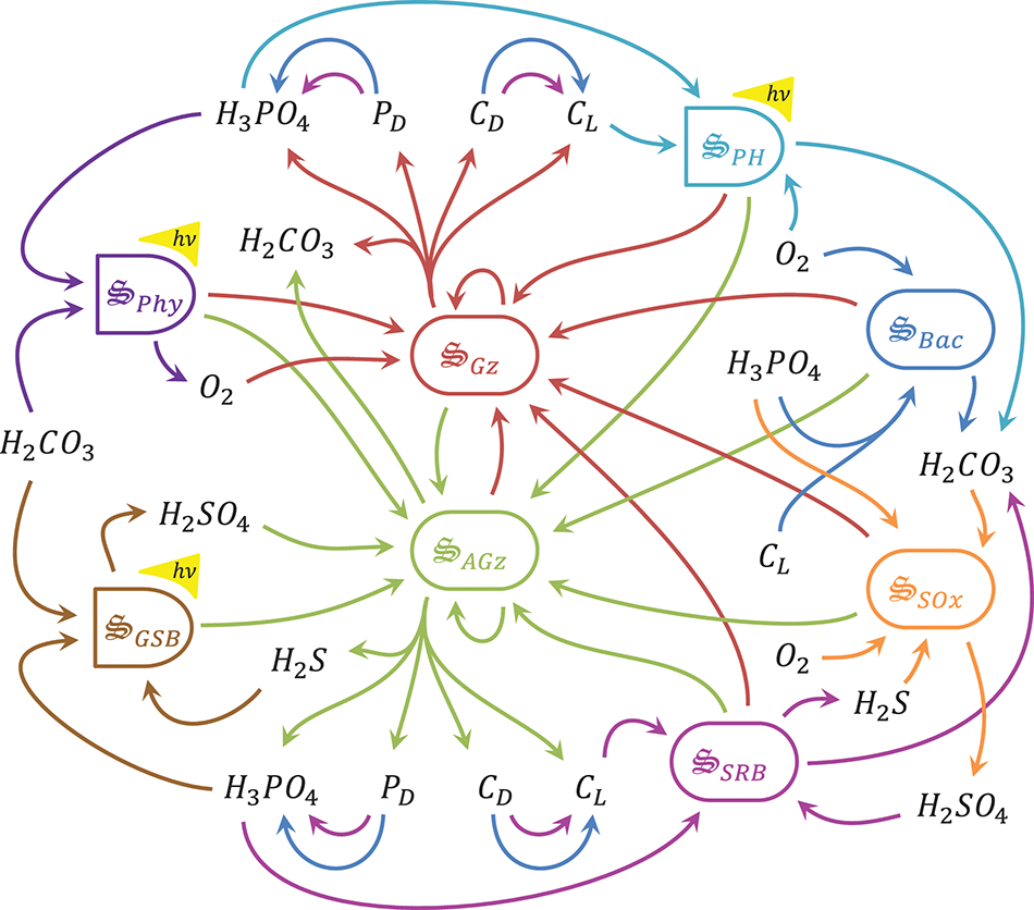
Schematic of catalysts and associated reactions used in the MEP model for Siders Pond. Functional groups include: , phytoplankton, purple, 2 rxns; , green sulfur bacteria, brown, 2 rxns; , aerobic grazers, red, 8 rxns; , anaerobic grazers, green, 8 rxns; , aerobic organoheterotrophic bacteria, blue, 3 rxns; , sulfate reducing bacteria, magenta, 3 rxns; , photoheterotrophs, cyan, 1 rxn; , sulfide oxidizing bacteria, orange, 1 rxn. Other abbreviations: hν, photon capture; CL, labile organic carbon; CD, refractory organic carbon; PD, refractory organic phosphorous. See Table 2 for qualitative representation of functional reactions and section 2.7 of the Supplementary Material for stoichiometrically balanced reactions.
Rationale
Our interest in investigating the applicability of MEP theory for describing microbial communities has, in addition to the basic science question, an applied objective. Standard models used to describe microbial biogeochemistry contain a large number of poorly constrained parameters, such as maximum growth rates, substrate affinity constants, growth efficiencies, prey preferences, substrate inhibition constant, and others. Consequently, data are required to determine parameter values, but since there is almost always more parameters than constraining observations, it is not difficult to obtain good agreement between model output and observations. Consequently, a good model fit does not equate to an understanding of the underlying mechanisms in a system. As a consequence, such models usually do poorly when extrapolated to different systems (Vallino, 2000; Ward et al., 2010). Parameters must be recalibrated for new conditions, but this defeats the purpose of developing a model, as we are often interested in using a model to predict how a system will respond to new conditions that have yet to occur. If the MEP principle fundamentally describes microbial communities, then models based on MEP should exhibit better extrapolation performance, since MEP would still be an appropriate objective function even under new conditions.
A challenging and unresolved aspect of MEP principle involves the temporal and spatial scales over which it applies (Dewar et al., 2014a). MEP theory has been developed for nonequilibrium steady-state systems where time is removed from the derivation, but natural microbial communities are dynamic and often far from steady state. For non-steady-state systems, we have proposed the following distinctions (Vallino, 2010). Abiotic processes, such as fire or a rock rolling down a hill, maximize instantaneous entropy production. That is, they follow a steepest descent trajectory down a potential energy surface in progress toward equilibrium, but this pathway can lead to metastable states that prevent further progress and entropy production. For instance, the flame gets extinguished or the rock gets stuck in a ditch partway down the hill. Biological systems, however, have evolved temporal strategies, such as circadian rhythms, that allow the system to take an alternate pathway that is not as steep, but it avoids metastable traps and enables further progress down the free energy surface. While instantaneous entropy production is lower in biological systems, when averaged over time, the integrated entropy production is greater than abiotic processes. Since MEP theory proposes that system configurations that produce more entropy are more likely to prevail (Lorenz, 2003), the higher average entropy production by biological systems allow them to persist over abiotic processes, at least in some situations. Similarly, when considering a spatial domain, entropy production can either be maximized locally at each point in the domain, or entropy production at each point can be adjusted so that entropy production is maximized globally over the entire domain. A simple numerical study indicated that when a system organizes over space, entropy produced by global optimization can exceed that from local optimization, but this requires spatial coordination by the community, while abiotic systems are likely to only maximize entropy production locally (Vallino, 2011). This paper will explore how changes in time and space scales over which entropy is maximized alters model predictions of microbial biogeochemistry. To provide some grounding in reality, model predictions are compared to biogeochemical observations. The purpose of this manuscript is to demonstrate one particular implementation of how MEP can be used to describe microbial biogeochemistry in natural systems that goes beyond a simple conceptual model, but ours is certainly not the only approach.
Methods
This section describes Siders Pond sample collection procedures and sample analyses followed by the development of the MEP model and associated 1D transport model for Siders Pond.
Siders pond
Site description
Siders Pond is a small coastal meromictic kettle hole (volume: 106 m3; area: 13.4 ha; maximum depth: 15 m) that receives approximately 1 × 10⁶ m3 of fresh and 0.15 × 10⁶ m3 of saltwater each year (Caraco, 1986). The latter input occurs via a small creek that connects the pond to Vineyard Sound approximately 550 m to the south. Tritium-helium water dating confirmed vertical mixing across two observed chemoclines, but permanent stratification is maintained because the saltwater inputs enter the pond at depth, mix upward and become entrained with freshwater before exiting the pond (Caraco, 1986). Caraco (1986) also characterized N and P loading to the pond (50 g N m2 y−1 and 1.3 g P m−2 y−1, respectively), and an N+P enrichment study (Caraco et al., 1987) showed phytoplankton to be P limited, especially in the low salinity surface waters. Previous studies show Siders Pond is eutrophic averaging 16 mg m−3 chlorophyll a (Chl a) in surface waters (but can exceed 100 mg m−3 at times) and an annual primary productivity of 315 g C m−2 (Caraco, 1986; Caraco and Puccoon, 1986). In anoxic bottom waters, bacterial Chl c, d and e associated with photosynthetic green sulfur bacteria averages 20 mg m−3 (purple sulfur bacteria were not found in high concentration), but BChl cde was also observed to reach high concentrations at times (> 75 mg m−3). Even though green sulfur bacteria could attain high concentrations, their productivity was only 6% of the oxygenic photoautotroph (cyanobacteria + algae) production (Caraco, 1986). Siders Pond was chosen for this study because extensive redox cycling occurs over a 15 m deep water column, which greatly facilitates sampling due to the large water volumes that can be readily collected without perturbing the system.
Sampling and measurements
Samples were collected from Siders Pond, Falmouth, MA over a 24 h period starting at 6:45 on Jun 25th and ending at 7:37 on Jun 26th, 2015 from a single station located within the deepest basin of the pond (41.548212°N, 70.622412°W). A total of 7 casts were conducted over the 24 hr period, and each cast sampled 8 depths to generate a 2D sampling grid designed for comparison to model outputs (Figure 2). A Hydrolab DS5 water quality sonde (OTT Hydromet, GmbH) was connected to a Hydrolab Surveyor 4 handheld display and used to record depth, temperature, salinity, pH, dissolved oxygen (DO), photosynthetic active radiation (PAR), and in situ Chl a fluorescence. All sensors were calibrated per manufacturer's instructions one day prior to sampling. One end of a 20 m long section of vinyl tubing with a 1 cm inside diameter was attached to the water quality sonde, while the other end passed through a Geopump 2 (Geotech, CO) peristaltic pump and then connected to 25 mm polypropylene, acid washed, in-line Swinnex filter holder (Millipore, MA), which housed a GF/F glass fiber filter (Whatman, GE Healthcare) that had been ashed at 450°C for 1 hr. At all depths, the vinyl tubing was first flushed for at least 2 min, sample collection vials were washed twice with filtrate and GF/F filters where changed as needed to maintain high flow. This design allowed water samples to be collected at the desired depths and processed on location then preserved on ice or dry ice for later analysis as described below.
Figure 2
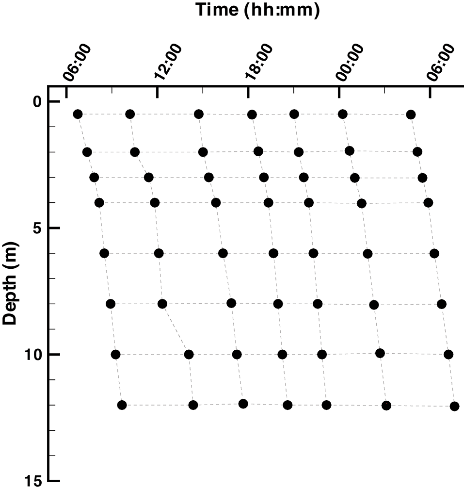
Layout of the Siders Pond 2D (t, z) sample grid. Samples were collected over a 24 h diel cycle starting at ~ 6:00 on 25 Jun 2015 and ending at ~6:00 on 26 Jun 2015. Samples were collected at 0.5, 2, 3, 4, 6, 8, 10, and 12 m.
Unless otherwise noted, all samples were filtered as described above and stored in 20 mL acid-washed, high-density polyethylene scintillation vials (Fisher Scientific). Samples were preserved for later analysis as follows. Inorganic phosphate: 15 mL samples were amended with 20 μL of 5 N HCl and placed on dry ice. Dissolved inorganic carbon (DIC) and sulfate: samples were collected in 12 mL exetainers (Labco, UK) by overfilling bottles from the bottom up, and then capped without bubbles and placed on ice. Hydrogen sulfide: while filling exetainers, 25 μL of sample was pipette transferred to 6 mL of 2% zinc acetate in a 20 mL scintillation vial and place on ice. Dissolved organic carbon (DOC): 25 mL of sample was collected in previously ashed 30 mL glass vials to which 40 μL of 5 N HCl was added then stored on ice. Particulate organic carbon (POC): approximately 300 mL of sample was passed through new, ashed, 25 mm GF/F filter then stored in a plastic Petri dish on dry ice.
Samples were analyzed at the Ecosystems laboratory, MBL as follows. Phosphate: samples were stored at −20°C then later analyzed following the spectrophotometric method of Murphy and Riley (1962) on a UV-1800 spectrophotometer (Shimadzu, Kyoto, Japan). DIC: samples were immediately run on return to MBL on an Apollo AS-C3 DIC analyzer (Apollo SciTech, DE). Sulfate: samples were sparged with N2 to strip H2S on return to MBL and stored at 4°C then analyzed using ion chromatography on a Dionex DX-120 analyzer (Dionex, Sunnyvale, CA). Hydrogen sulfide: samples were briefly stored at 4°C for 5 days then analyzed using the spectrophotometric method of Gilboa-Garber (1971). DOC: samples were stored at 4°C then run on a Shimadzu TOC-L high temperature total organic carbon analyzer at 720°C. POC: samples were stored at −20°C then analyzed on a Thermo Scientific FLASH 2000 CHN analyzer using aspartic acid standards. To facilitate model comparison to observations, Chl a was estimated from modeled output of phototroph biomass concentrations using , where θC:Chla is the C:Chl a ratio, which was set to 50 μg C (μg Chl a)−1 (Sathyendranath et al., 2009).
Model development
The equations used to model biogeochemistry in Siders Pond are provided in detail in the Supplementary Material, so the descriptions in this section focus primarily on model concepts that form the basis of the modeling approach and extensions to previous studies. The model consists of three main components: (1) a set of biologically catalyzed reactions that constitute the distributed metabolic network of the microbial community, including predators such as protist and viruses; (2) a 1D transport model; (3) an optimization component in which control variables that govern reaction stoichiometry, kinetics and thermodynamics are determined so as to maximize internal entropy production over a specified interval of time and space. We describe briefly below the three model components, but we focus first on the representation of the metabolic network, as this forms the foundation of the approach, and includes the concentrations of 11 chemical constituents and 8 functional groups (Figure 1, Table 1).
Table 1
| Variable | Sym. | Variable | Sym. |
|---|---|---|---|
| Salt | cSal | Phytoplankton | |
| Dissolved oxygen | cO2 | Green sulfur bacteria | |
| Dissolved inorganic carbon | cH2CO3 | Aerobic predators | |
| Inorganic phosphate | cH3PO4 | Anaerobic predators | |
| Sulfate | cH2SO4 | Aerobic organoheterotrophic bacteria | |
| Hydrogen sulfide | cH2S | Sulfate reducing bacteria | |
| Phytoplankton carbohydrates | cCPhy | Photoheterotrophs | |
| Green sulfur bacteria carbohydrates | cCGSB | Sulfide oxidizing bacteria | |
| Labile organic carbon | cCL | ||
| Refractory organic carbon | cCD | ||
| Refractory organic phosphate | cPD |
Names of state variables and associated symbols.
All state variables represent concentrations in mmol m−3, except for salt, which is in PSU. Concentrations of NH3 (cNH3) and detrital N (cND) are included in chemical reactions for stoichiometric and thermodynamic calculations, but were held constant at 5 and 10 mmol m−3, respectively, in all simulations.
Catalysts and metabolic reaction network
Our approach views a complex microbial community as a collection of catalysts (denoted with the special symbol with the subscript j meaning any of the 8 functional groups in Figure 1) that each have a subset of nr, j functional reactions they catalyze. The catalyst has an elemental composition given by . For this study all catalysts are assigned the same composition as yeast with associated thermodynamic properties (Battley et al., 1997), but this is not an overly constraining approximation (Vallino et al., 2014) and can be easily relaxed if needed. The catalysts and reactions included in the metabolic network represent the capabilities of the entire microbial community, but the reactions are distributed across catalysts (8 for the case of Siders Pond, Figure 1), just as functions are distributed across phyla in natural communities (Vallino, 2003). The reactions are highly simplified and condensed, and consist of two essential components: an anabolic reaction that synthesizes catalyst from environmental resources, and a catabolic reaction that provides free energy to drive the anabolic reaction forward. A highly simplified list of metabolic reactions for the Siders Pond model is given in Table 2. To convey the basic ideas, we consider below the phyla responsible for sulfate reduction for chemotrophy and phytoplankton for phototrophy.
Table 2
| Rxn. | Abbreviated Stoichiometry | Cat. |
|---|---|---|
| r1, Phy | H2CO3+hν→CPhy+O2 | |
| r2, Phy | ||
| r1, GSB | H2CO3+H2S+hν→CGSB+H2SO4 | |
| r2, GSB | ||
| r1−8, Gz | ||
| r1−8, AGz | ||
| r1, Bac | ||
| r2, Bac | CD→CL | |
| r3, Bac | PD→H3PO4 | |
| r1, SRB | ||
| r2, SRB | CD→CL | |
| r3, SRB | PD→H3PO4 | |
| r1, PH | ||
| r1, SOx |
Reactions associated with the 8 biological catalysts, , used to model microbial biogeochemistry in Siders Pond, where ri, j represents sub-reaction i of biological catalyst .
There are a total of 28 reactions, where and each catalyzed 8 sub-reactions. Reactions are shown to emphasize function only. Complete reaction stoichiometries, including influence of optimal control variables, are given in section 2.7 of the Supplementary Material. See caption of Figure 1 for nomenclature.
Chemotrophyh
The catalyst represents the capabilities of sulfate reducing bacteria (SRB) that oxidize labile organic matter, CL, using sulfate as the electron acceptor. The anabolic and catabolic reactions are given by,
respectively, where the stoichiometric coefficients, and , are determined from elemental balances around O and H. Both reactions above must be catalyzed by , so the reaction rates are proportional to the concentration of the catalyst, , present (note, we also use bracket nomenclature, , for concentration below). These two reactions can be combined by introducing a reaction efficiency variable, εSRB, to produce an overall reaction representing growth and respiration of sulfate reducing bacteria, r1, SRB, given by,
The reaction efficiency variable, εSRB, is one of two classes of optimal control variables and a central design feature of the MEP model. As εSRB approaches 1, Equation (3) represents 100% conversion of labile carbon plus N and P resources to catalyst, while as εSRB approaches 0, the reaction changes to 100% anaerobic combustion of labile carbon. From an entropy production perspective, only the catabolic reaction dissipates significant free energy, so εSRB should be set to zero to maximize entropy production; however, the catabolic reaction cannot proceed without catalyst. There exists, then, an optimum value of εSRB that produces just enough catalyst to dissipate the chemical potential between CL and H2SO4, but εSRB must change as a function of CL and H2SO4 supply rates as well as N and P availability. Conceptually, the MEP problem is to determine how εSRB should change over time and space to maximize free energy dissipation; however, there are a few other important details.
Gibbs free energies of reaction, ΔrGi, j, are calculated using Alberty's (2003) approach, which accounts for substrate activities, pH and temperature. For chemotrophic reactions, an adaptive Monod equation parameterized by εj accounts for the tradeoffs between substrate affinity, maximum specific growth rate and growth efficiency and can approximate oligotrophic to copiotrophic growth kinetics by varying εj between 0 and 1 (Algar and Vallino, 2014; Vallino et al., 2014). In addition to this kinetic constraint, FK, reaction rates, ri, j, are also constrained by reaction thermodynamics, FT, as described by La Rowe et al. (2012). Consequently, the rates of chemotrophic reactions take the following general form,
where c are substrate concentrations, ν* and κ* are universal constants and Ωi, j is the second optimal control variable class. Since each catalyst, , can catalyze nr, j sub-reactions (Table 2), Ωi, j determines the fraction of catalyst j, , that is allocated to reaction ri, j. For instance, the sulfate reducing bacteria have two others reactions in addition to r1, SRB, Equation (3) (Table 2). Reactions r2, SRB and r3, SRB allow SRB to decompose recalcitrant organic carbon, CD, and phosphorous, PD, into labile organic carbon, CL, and inorganic phosphate, respectively, and Ωi, SRB determines the fraction of protein allocated to each of the three reactions. Consequently, each Ωi, j is bound between 0 and 1, and Ωi, j must sum to unity over all i for each catalyst; that is, . An example of how FK, ΔrGi, j, and FT vary over time and space to influence reaction rates of sulfate reducing bacteria is given in Supplementary Material 4.1, Figure S3.
Phototrophy
In this version of the MEP model we introduce catalysts associated with phototrophic growth, specifically phytoplankton (Phy), , anaerobic green sulfur bacteria (GSB), , and photoheterotrophs (PH), . Both Phy and GSB are modeled similarly using two sub-reactions (Table 2). One sub-reaction couples photon capture that drives CO2 fixation into carbohydrates, CPhy and CGSB, and a second sub-reaction converts carbohydrates into biomass in a manner analogous to growth of chemotrophs described above. We focus on phytoplankton here because development for GSB is similar, and can be found in the Supplementary Material.
The carbon fixation reaction for phytoplankton is given by,
where hν are captured photons of frequency ν, h is Plank's constant and n1, Phy is the moles of photons needed to fix 1 mole of CO2 at 100% efficiency (i.e., εPhy = 1). The Gibbs free energy for a mole of photons is given by
where NA is Avogadro's number and ηI is the thermodynamic efficiency for converting electromagnetic radiation into work (Candau, 2003). If ΔrGCPhy is the Gibbs free energy for fixing a mole of H2CO3 into CPhy plus O2, then moles of photons needed to fix 1 mole of CO2 is given by,
and the Gibbs free energy of reaction for CO2 fixation defined by Equation (5) is given by,
In this formulation, εPhy governs the efficiency for the conversation of electromagnetic potential into chemical potential. If 100% of photosynthetic active radiation is converted to chemical potential, no entropy is produced, and the free energy of reaction for Equation (5) is zero, so the reaction will not proceed due to thermodynamic constraints. However, as εPhy is decreased, some photons are dissipated as heat, which drives the reaction forward, and all photons are dissipated as heat when εPhy = 0, but no catalyst is synthesized.
The reaction rate for CO2 fixation depends on the rate of photon capture, which is given by,
where kp is the coefficient for light absorption by particles, is the fraction of phytoplankton catalytic machinery allocated to capturing photons (i.e., chlorophyll and electron transfer proteins), and I(t, z) is light intensity (mmol photons m−2 d−1) at time t and depth z. Consequently, the reaction rate for CO2 fixation is given by,
where FK and FT are the kinetic and thermodynamic drivers, respectively. This reaction has similarities to those typically used to describe phytoplankton growth (Macedo and Duarte, 2006), but our derivation focuses not on the local light intensity level, but rather on how much light is actually intercept by the phytoplankton, as governed by , and how much of that free energy is actually used to drive carbon fixation, as governed by εPhy. As evident in Equation (10), the maximum rate is directly tied to the rate of photon interception, ΔIPhy, not by an arbitrary maximum specific growth parameter. The second reaction used by Phy and GSB (Table 2) is simply the conversion of reduced organic carbon, CPhy and CGSB, into more catalyst or CO2 depending of the value of εPhy.
The reaction for photoheterotrophs (PH) differs slightly from that above. In this case only one reaction is used (r1, PH, Table 2), where photon capture is linked to the conversion of labile carbon into PH catalyst. As above, photons captured can also be dissipated as heat for εPH < 1, or the free energy can be used to drive biosynthesis (εPH > 0), where photon free energy replaces chemical free energy used in chemotroph reactions.
Transport model
Siders Pond is horizontally well mixed, so an advection-dispersion-reaction (ADR) model that includes particle sinking was used to approximate vertical transport of the 19 state variables (Figure 1). The origin of the vertical coordinate, z, is defined at the pond's surface, and the axis points in the positive direction downward toward the benthos and reaches a maximum depth of 15 m. Siders Pond 3D bathymetry surface was rendered from a contour plot in Caraco (1986), and an equation for cross-section area as a function of depth was derived therefrom (Figure S1). Equations for vertical volumetric flow rate, lateral groundwater inputs and seawater intrusion at the bottom boundary were derived from Caraco (1986), who used both tritium-helium-3 dating combined with mass balance calculations to estimate freshwater inputs and seawater intrusion. An equation for the dispersion coefficient was derived by fitting simulated salinity profiles to observations collected during this study.
The primary external drivers in the model are temperature, pH and photosynthetic active radiation. Surface irradiance was based on a model of solar zenith angle (Brock, 1981), which assumes a cloudless sky. To predict PAR light intensity as function of time and depth, a standard light adsorption model was used that includes coefficients for light absorption by water, kw, and particulate material, kp.
Neumann boundary conditions were used for state variables at the pond's surface and gas transport for O2, CO2, and H2S across the air-water interface was accounted for using a stagnant-film model. Robin boundary conditions were used for the bottom boundary based on the flux of material entering the boundary associated with the intrusion of seawater diluted with groundwater. In addition, aerobic and anaerobic decomposition of sinking organic matter from the water column contributed to a sink for O2 and H2SO4, and a source for H3PO4, H2CO3, and H2S to the overlying water.
Entropy production and optimization
Entropy-production
Entropy production occurs when an energy potential is destroyed and dissipated as heat to the environment, but not when the potential is converted to another potential. For example, a flame converting chemical potential into heat or light being absorbed by water both result in maximum entropy production; these are irreversible processes and the Gibbs free energy is destroyed. On the other hand, entropy is not produced if electromagnetic potential is converted reversibly into chemical potential, but thermodynamic theory requires that reversible reactions must proceed infinitely slowly. In the model, as the reaction efficiency for phytoplankton, εPhy, approaches 1, electromagnetic potential is converted to chemical potential without entropy production, but the thermodynamic force, FT, drivers the reaction rate to 0, and as εPhy approaches zero, all electromagnetic potential is dissipated as heat, but no catalyst is produced, as evident in Eq. (5). Consequently, living organisms operate between these two extremes. For organisms to grow at a non-zero rate, an energy potential must be partially dissipated and some entropy must be produced.
Instantaneous entropy production per unit volume, for chemotrophic reactions is readily calculated as the product of reaction rate times Gibbs free energy of reaction (Vallino, 2010) divided by temperature, T, as given by,
Average entropy production, , is calculated by integrating over an interval of time, Δt, as given by,
The value of △t is unknown, but it is the fundamental parameter of interest in this study, because it represents the time scale over which biology has evolved to operate.
Entropy production associated with the dissipation of electromagnetic radiation is readily calculated from the Gibbs free energy for photons, Equation (6), and photon capture rate, Equation (9). The photon free energy can be dissipated as heat along two pathways: (1) interception by water or (2) particles, such as bacteria and grazers, as well as by the non-photosynthetic components of phytoplankton. Photons intercepted by the photosynthetic machinery of phototrophs can be either dissipated as heat, if εj = 0, or all energy potential can be transferred to chemical potential, if εj = 1, but typically it is a combination of both, so that 0 < εj < 1. Consequently, total entropy production, , is the sum of three processes: entropy production by light absorption by water, , entropy production by light absorption by particles, , and entropy production by chemical reactions, , including photoreactions. All entropy production terms are accounted for in the MEP optimization problem, including that from light absorption by water and particles.
MEP-optimization
The stoichiometry, thermodynamics and kinetics of the 28 reactions that comprise the metabolic network (Table 2, Figure 1) vary as a function of the eight εj optimal control variables, and the partitioning of biological structure, , to sub-reactions ri, j that depends on the values of the Ωi, j control variables, of which there are 20. A solution to the MEP model, and associated microbial biogeochemistry, is determined by adjusting εj and Ωi, j over △t time and 1D space to maximize entropy production, the details of which are provided in Supplementary Material section 3.2, but also see Vallino et al. (2014). As △t approaches 0 in Equation (12), the average entropy production, , approaches the instantaneous value, , and describes abiotic processes based on our hypothesis. Increasing △t permits other solutions that are not constrained to the steepest descent trajectory. By changing values of εj and Ωi, j over time and space, pathways that avoid the ditch halfway down the hill are allowed, or strategies that anticipate the sun rising in the morning can be exploited. The critical aspect of the optimization is choosing the appropriate time interval over which to maximize entropy production and whether local or global optimization should be used (Vallino, 2011); consequently, these two aspects are the focus of this manuscript and form the bases of the Results section.
Physical parameters and model skill assessment
If the MEP model developed here were cast as a conventional biogeochemistry model, there would be 89 biological parameters associated with growth kinetics. Instead, there are 28 optimal control (OC) variables (8 εj and 20 Ωi, j), but only one biological parameter, because the OC variables are determined by maximizing entropy production described above. The sole biological parameter, Δt, specifies the time scale over which entropy is maximized, Equation (12), and its impact on solution dynamics is the focus of this manuscript. There are 11 uncertain physical parameters, 9 associated with particulate matter sinking velocities and two associated with light absorption by water and particles. Since fitting model output to observations is not an indication of good model forecasting fidelity, we only crudely adjusted the 11 physical parameters so that model outputs were within an order of magnitude of observations. These adjustments were made with fix values of the 28 OC variables that were set arbitrarily. The objective was to get the physics to reasonably approximate that occurring in Sider Pond.
To determine model performance, 2D linear interpolation was used to extract values of model state variables at times and depths corresponding to those taken for observations. Root mean squared errors were then calculated between interpolated model outputs and observations to quantify model skill (Fitzpatrick, 2009). The computational approach used for solving the 1D advection-dispersion-reaction equation is described in Supplementary Material section 2.9 and the approach used for solving the optimal control problem is described in Supplementary Material section 3.2.
Results
All solutions presented here are from local entropy maximization at 10 depths (0, 1, 2, 3, 4, 6, 8, 10, 12, and 15 m). We investigated two optimization time intervals, △t, for entropy maximization, a short interval of 0.25 days and a long interval of 3 days. Simulations were started on May 19th, but only the last 6 days of simulations from Jun 21st to Jun 27th are shown here and compared to observations collected on Jun 25th and 26th (Figure 2). Our results focus on how these two solutions compare to observations in the Simulations Compared to Observations section as well as how the short and long interval optimization windows differ from each other in the Comparison Between SIO and LIO Simulations section.
Simulations compared to observations
Solutions obtained from the short (0.25 day) and long (3 day) interval optimizations are compared to biogeochemical observations from Siders Pond that were collected to form a 2D sample grid on Jun 25th and 26th, 2015 (Figure 2). Simulated profiles for photosynthetic active radiation (PAR), Chl a and dissolved oxygen (DO) are compared to observations in Siders Pond in Figure 3. The short interval optimization (SIO) shows PAR extending to nearly the bottom of the pond (Figure 3A), while PAR from the long interval optimization (LIO) (Figure 3B) more closely matches observations (Figure 3C). The prediction for Chl a in both simulations do not match observations very well (Figures 3D–F), but this is partially due to how Chl a was estimated, since Chl a is not specifically modeled. The Chl a in vivo observations show a peak Chl a around 5 m, while both simulations have peaks around 12 m, but those peaks are due to accumulation of sinking phytoplankton rather than productivity at that depth. The LIO simulation does show a secondary Chl a peak developing around 3 m, but it is weaker than observations (~ 6 vs. 40 μg L−1). Based on DO, the SIO shows anaerobic conditions begin at 6 m, while the LIO shows that occurring at 10 m. The observed transition to anoxia splits between the two simulations at 8 m. Observations also show a subsurface DO maximum at 3.5 m, while both simulations show max DO closer to 1.3 m. Furthermore, the SIO shows a decreasing DO max with time, while the LIO shows an increase over time, and the maximum reaches 800 mmol m−3 vs. 480 for observations. In general, the SIO simulations show less phototrophic activity while LIO shows greater activity than what the observations indicate. The LIO solutions show better fits to observations for PAR and Chl a based on RMSE, while the SIO shows a better fit to DO (Table 3).
Table 3
| △t (d) | PAR (μE m−2 s−1) | Chl a (μg L−1) | DO (μM) | H3PO4 (μM) | DIC (μM) | H2S (μM) | H2SO4 (μM) | DOC (μM) | POC (μM) |
|---|---|---|---|---|---|---|---|---|---|
| 0.25 | 484. | 32.9 | 137. | 4.69 | 6050. | 2500. | 3650. | 388. | 167. |
| 3.00 | 189. | 24.4 | 212. | 4.88 | 5610. | 2280. | 3390. | 361. | 198. |
Root mean squared errors between model predictions and observations for the short (SIO, t = 0.25 d) and long (LIO, t = 3.0 d) interval optimizations.
Better (i.e., lower) scores are highlighted in bold italic font face.
Figure 3
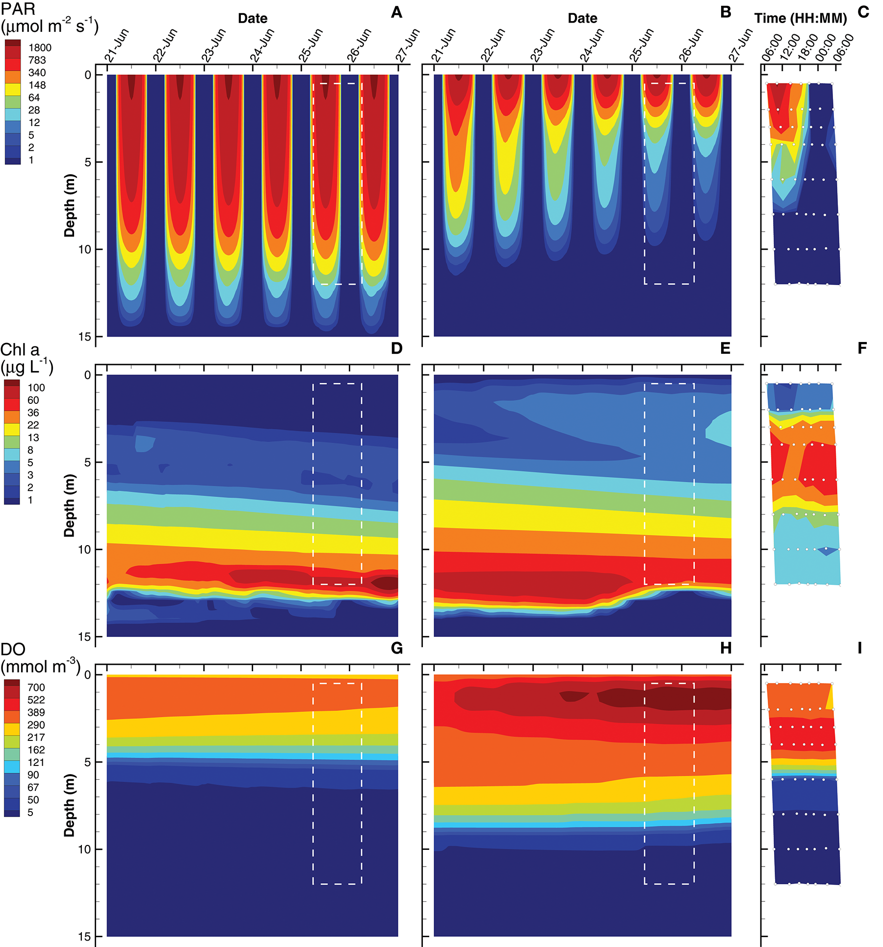
Contour plots of photosynthetic active radiation (PAR) (A–C), chlorophyll (Chl) a concentration (D–F) and dissolved oxygen (DO) (G–I) for six day simulations using short interval optimization (SIO) (left column), long interval optimization (LIO) (center column) and for observations collected from Siders Pond over a 24 h period on Jun 25 to Jun 26 2015 (right column). Rectangle (dashed white lines) in simulation plots corresponds to time and depths where observations are comparable (i.e., Jun 25/26, 0.5 to 12 m). Actual observations are shown as white circles with black perimeters (see also Figure 2).
Simulations of substrate concentrations for autotrophs, namely inorganic phosphate and dissolved inorganic carbon (DIC), show qualitative agreement to observations for both SIO and LIO solutions (Figure 4), but some discrepancies are apparent. The phosphate chemoclines occur around 10, 11, and 8 m for the SIO, LIO, and observations, respectively (Figures 4A–C). Above the phosphate chemocline, the SIO simulation shows slightly elevated levels of H3PO4 (~0.3 mmol m−3) in the surface and 5 m layers, compare to observations (Figure 4C), which are near the level of detection (0.03 mmol m−3) except for a few spikes. Below the phosphate chemocline, observations show slightly higher accumulations of phosphate, approaching 22 mmol m−3, while the SIO and LIO simulations show max concentrations closer to 16 and 19 mmol m−3, respectively. For DIC, both SIO and LIO simulations show much lower DIC concentrations below 10 m (3,000 and 5,400 mmol m−3, respectively) than observed in Siders Pond (16,500 mmol m−3), which would indicate much higher anaerobic remineralization in the pond than occurs in the simulations. The SIO and LIO also show greater draw down of DIC in the surface water above 2 and 4 m respectively, and the LIO simulation shows minimum DIC approaching just 2 mmol m−3 at 1 m, while minimum observed value is above 660 mmol m−3. The SIO simulation fits phosphate observations slight better than the LIO simulation, but LIO does better at fitting the DIC observations (Table 3).
Figure 4
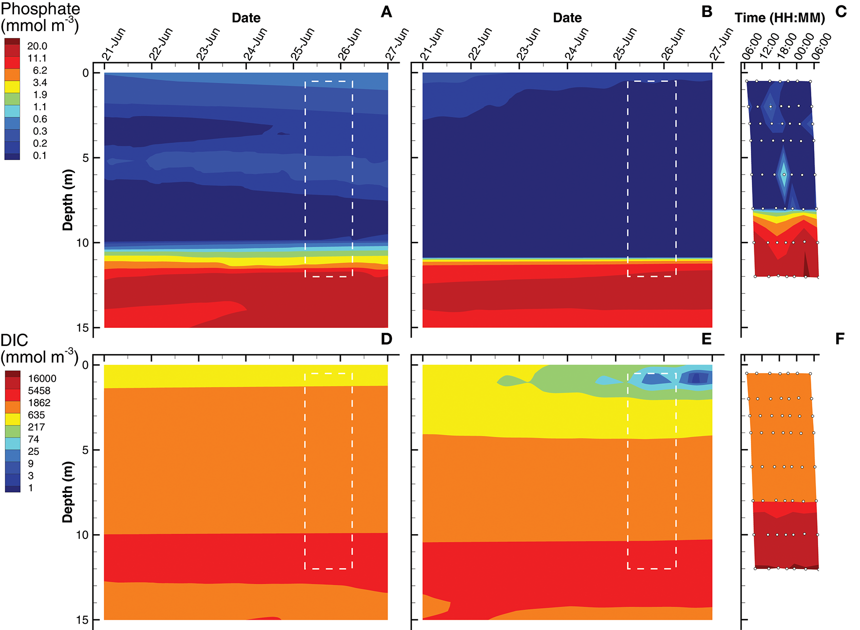
Contour plots of inorganic phosphate (A–C) and dissolved inorganic carbon (DIC) (D–F) concentrations for SIO and LIO simulations (left and center columns, respectively) and Siders Pond observations (right column). See caption to Figure 3 for other details.
Simulations of hydrogen sulfide show a chemocline at approximately 9 and 10 m for the SIO and LIO solutions, respectively, which are slightly deeper than the H2S chemocline observed in Siders Pond at about 8 m (Figures 5A–C). However, H2S reaches concentrations as high as 7,000 mmol m−3 in Siders Pond, while maximum concentrations only reach 900 and 2,100 mmol m−3 in the SIO and LIO simulations, respectively. Simulations also show a peak H2S concentration at 12 m, and a decrease in concentration below 12 m, which also indicates lower anaerobic respiration in the simulations. Simulated sulfate concentrations in the upper portion of the water column (0 to 4 m) are similar to those observed (Figures 5D,E), but the simulations show an abrupt sulfate chemocline starting at about 8 m, while observations show a more gradual increase in sulfate with depth. Furthermore, sulfate reaches much higher concentrations in the simulations at depth than do observations, showing maximums of 15,500 mmol m−3 in both simulations, while observation maximum is only 9,000 mmol m−3. The lower simulated concentrations of H2S and the higher simulated sulfate concentrations indicate that sulfate reduction in the model is lower than that actually occurring in Siders Pond, but the LIO simulations fit observations better for both H2S and H2SO4 than do the SIO simulations (Table 3).
Figure 5
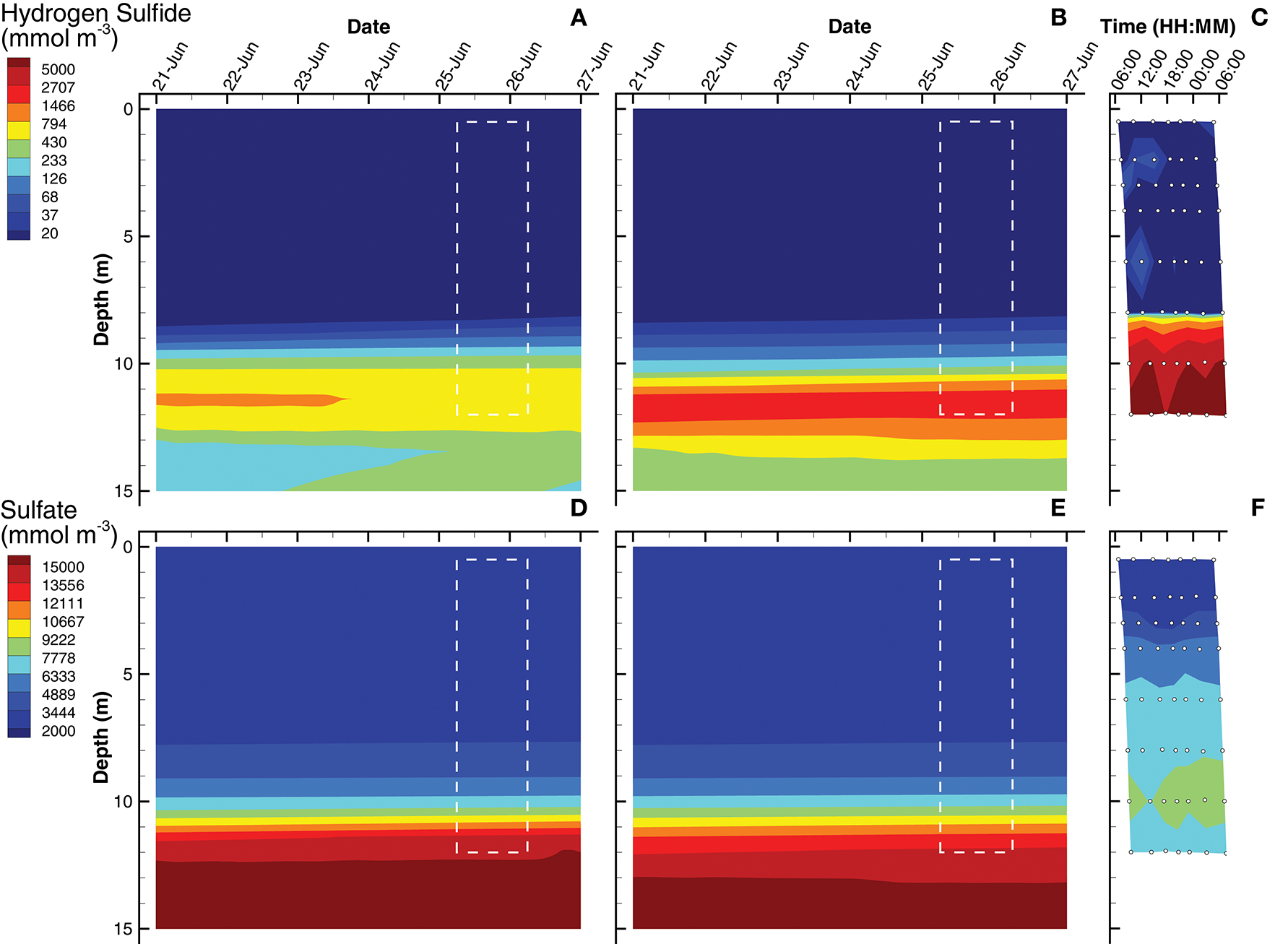
Contour plots of hydrogen sulfide (A–C) and sulfate (D–F) concentrations for SIO and LIO simulations (left and center columns, respectively) and Siders Pond observations (right column). See caption to Figure 3 for other details.
The last of the observations are dissolved organic carbon (DOC) and particulate organic carbon (POC) concentrations (Figure 6). For simulations, DOC is a derived quantity based on the sum of state variables [CL] and [CD], while POC is derived from the sum of internal carbohydrate stores, [CPhy] and [CGSB], plus the concentrations of all biological structures, . In the water column above 12 m, the SIO simulation shows very low concentrations of DOC (~ 1 mmol m−3), but then increases rapidly to a maximum of 1,900 mmol m−3 (Figure 6A). The LIO simulation shows a similarly high DOC concentration at 14 m, but above 12 m, the DOC concentration ranges from 2 to 140 mmol m−3, which is closer to those observed in Siders Pond, which range from 200 to 300 mmol m−3 above 10 m, and increase to a maximum of about 1,000 mmol m−3 at 12 m. Similar to DOC, POC in the SIO simulation shows low values (< 30 mmol m−3) above 6 m, but POC peaks to 1,000 mmol m−3 at 12 m (Figure 6D). The POC concentrations from the LIO simulation are closer to observations, but the mid-water POC maximum in the LIO simulation is approximately 500 mmol m−3, while the observations peak at 280 mmol m−3 around 4 m. Like the SIO simulation, the LIO simulation also shows high POC concentrations below 10 m, which was not observed in Siders Pond. It is possible that DOC and POC may reach higher concentrations in the funnel-like basin of Siders Pond below 12 m, but samples were not collected there. While the LIO simulations show better fit to DOC observations, the SIO simulations fit the POC observations better (Table 3). Overall, the LIO simulations fit six observations better, while the SIO simulations of fit three observations better, which indicates the LIO simulations are overall closer to observations (Table 3). On a qualitative measure, the LIO simulation produces a phytoplankton bloom near the surface of the pond (Figure 3), which is consistent with multiple years of student collected observations from Sider Pond. In that regard, the LIO solution appears better at predicting this important feature of Siders Pond.
Figure 6
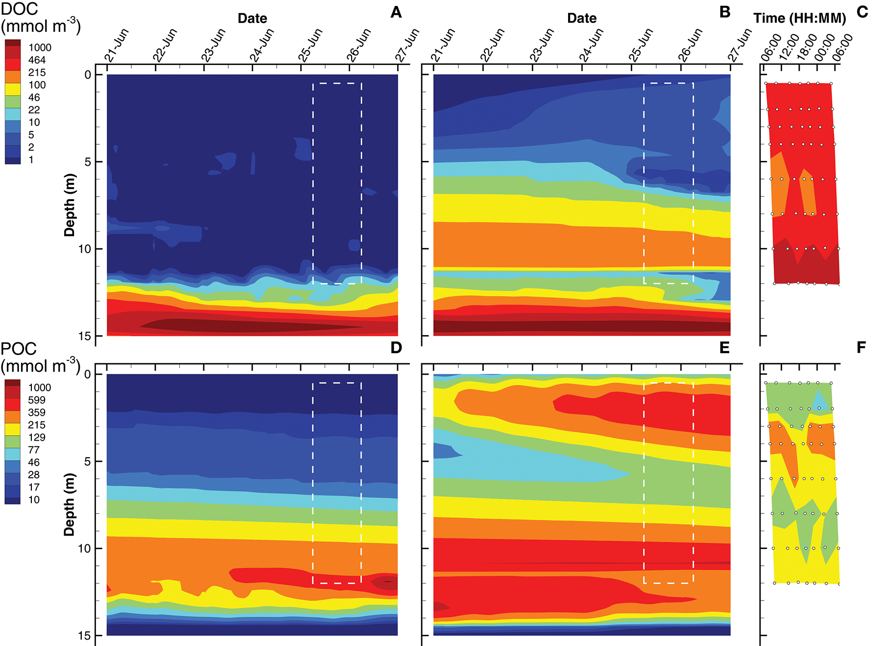
Contour plots of dissolved organic carbon (DOC) (A–C) and particulate organic carbon (POC) (D–F) concentrations for SIO and LIO simulations (left and center columns, respectively) and Siders Pond observations (right column). See caption to Figure 3 for other details.
Comparison between SIO and LIO simulations
Since the MEP optimization model generates a large number of outputs, this section highlights some of those outputs to contrast the simulations based on the short (0.25 d) interval optimization (SIO) to that from the long (3 d) interval optimization (LIO). Consider entropy production, which is the variable that is being sequentially maximized over a 0.25 d interval (SIO) or a 3 d interval (LIO) at 10 different depths (Figure 7). Total entropy production, , for the SIO and LIO simulations differ significantly, in that in the SIO solution is spread out over a 12 m water column (Figure 7A) vs. the LIO solution (Figure 7E), where most of the entropy production occurs in the top 3 m of the pond. Furthermore, peak entropy production in the LIO simulation is 7.5 times great than the SIO solution (9.8 vs. 1.3 GJ m−1 K−1 d−1), and the total integrated entropy produced over the water column and over the 6 day simulation, σT, was 21.3 GJ K−1 and 36.5 GJ K−1 for the SIO and LIO simulations, respectively. For comparison, if the pond was sterile, σT would equal 12.4 GJ K−1 from light absorption in the water column. The 71% higher total integrated entropy, σT, produced by the LIO simulation illustrates that extending the optimization time scale results in greater entropy production, which is consistent with a previous study (Vallino et al., 2014).
Figure 7
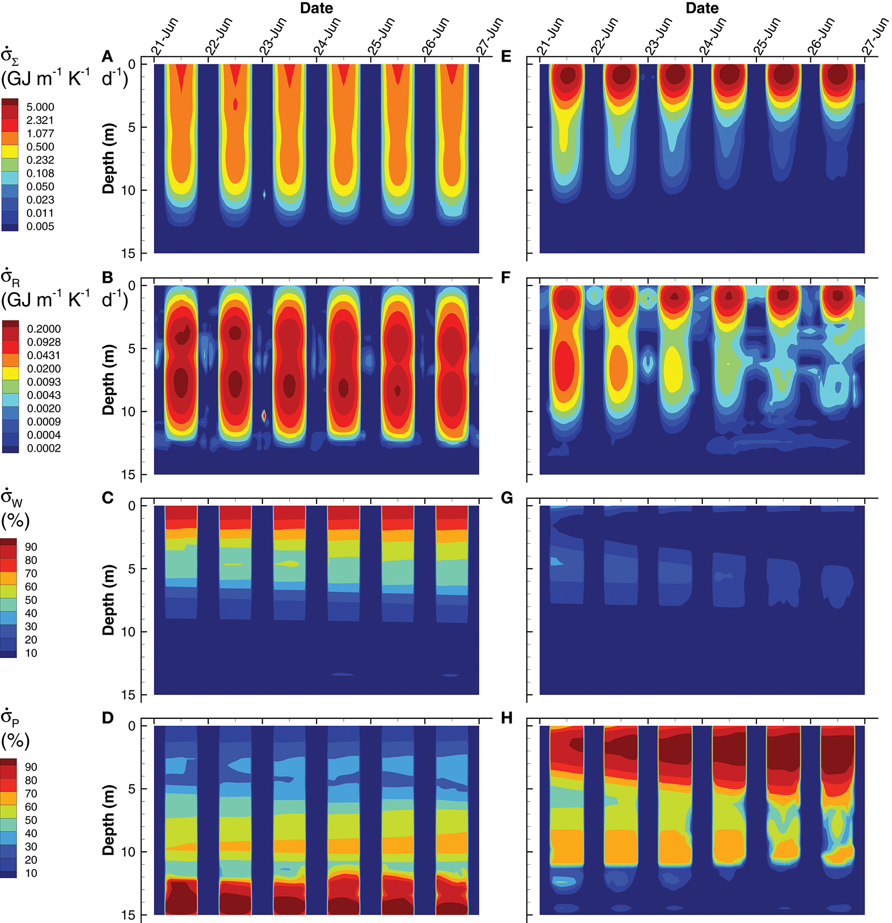
Contour plots of simulated total entropy production, (Eq. (S178)) (A,E), entropy production from reactions, [Equation (S178)] (B,F), and entropy production from light absorption by water, [Equation (S176)] (C,G) and particles, [Equation (S177)] (D,H) for the SIO (left column) and LIO (right column) simulations. Entropy production from light dissipation by water and particles are shown as a percentage of total entropy production.
The different contributors to total entropy production, namely by reaction, , water, , and particles, , also differ significantly between the two simulations. For instance, total integrated entropy production associated with reactions was actually greater in the SIO than the LIO simulation (Figure 7B vs. Figure 7F), as well as exhibited a greater maximum (0.28 vs. 0.26 GJ m−1 K−1 d−1 for SIO versus LIO); however, entropy production by reaction during the day is rather small (< 25% in the upper 5 m) compared to light dissipation by water or particles, but the two simulations differ here as well. The SIO simulation dissipates most of the incoming radiation by water absorption in the upper 5 m of the water column (Figure 7C vs. Figure 7G), while the LIO simulation dissipates most of the electromagnetic potential via absorption by particles (Figure 7D vs. Figure 7H). As evident in the POC (Figure 6) and Chl a (Figure 3) concentrations, the LIO simulation produces more biomass in the upper portion of the water column, and biomass is effective at absorbing and dissipating light.
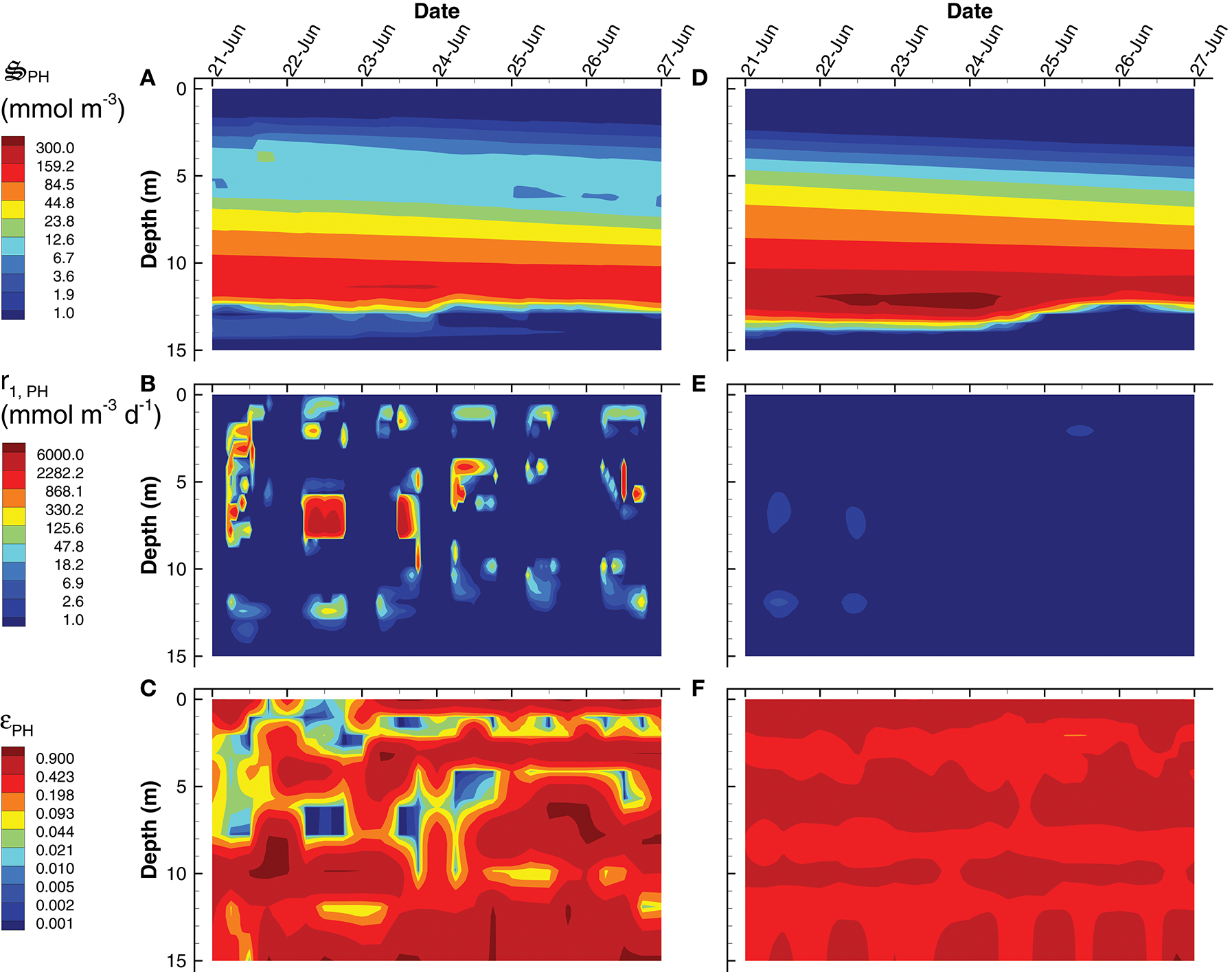
An analysis of phytoplankton (Phy) growth by the SIO and LIO simulations (Figure 8) illustrates not only how the two simulations differ, but also some of the mechanics of the MEP-based optimization approach. Phytoplankton density attains a maximum of 20 mmol m−3 in the LIO simulation by June 27th, but Phy are effectively absent in the SIO simulation, attaining a maximum of only 0.1 mmol m−3 (Figures 8A,F). While it is possible that the low phytoplankton density in the SIO simulation could be due to extensive predation, this is not the case because the rates of CO2 fixation (r1, Phy, Table 2) and conversion of fixed C to biomass (r2, Phy, Table 2) are two orders of magnitude lower in the SIO versus LIO simulation (Figures 8B,C vs. Figures 8G,H). The differences in phytoplankton density and reaction rates between the SIO and LIO simulations are due to how the optimal control variables change over time and space (Figures 8D,E,I,J). Consider how reaction efficiency, εPhy, varies over time and space in the two simulations (Figures 8D,I). The SIO simulation shows rapid switching between very high efficiencies (>0.98) and very low efficiencies (< 0.02) over time. While not on all days, reaction efficiency drops to very low levels around noon (Figure 8D), which results in high entropy production, but at the sacrifice of fixing CO2, which is consistent with maximizing energy dissipation on a short term time scale. On the contrary, the LIO solution (Figure 8I) shows more gradual changes in εPhy, operating between 0.3 and 0.4 for most of the simulation. There is rapid changing of the biomass allocation variable, Ω1, Phy, in the LIO solution (Figure 8J), but this makes sense, because the control variable partitions phytoplankton biomass to the light requiring carbon fixation reaction, r1, Phy, during peak daylight (Figure 8G), then switches to the biosynthesis reaction, r2, Phy, at night (Figure 8H). Based on Figure 7C, the SIO solution instead uses water for the short term dissipation of electromagnetic potential in the pond's surface, but in deeper water the SIO solution does produce biomass.
Figure 8
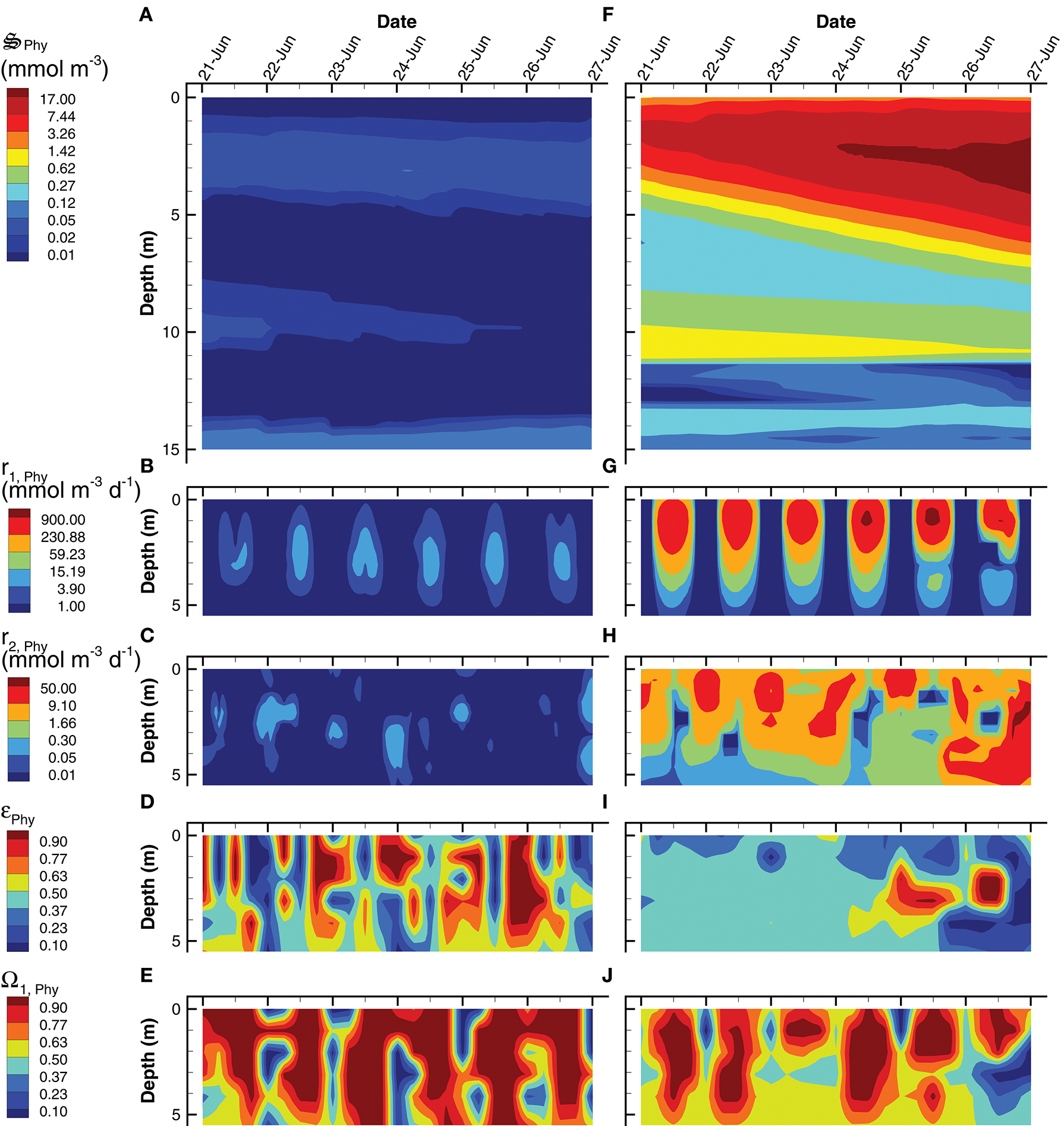
Contour plots of phytoplankton concentration, (A,F), rates for the two associated reactions, r1, Phy(B,G) and, r2, Phy(C,H) and two optimal control variables, εPhy(D,I), and Ω1, Phy(E,J) for the SIO (A–E) and LIO (F–J) simulations. Note, reaction rates and control variables are only plotted for the top 5 m of the water column where the processes are significant.
Instead of producing phytoplankton, the SIO solution produces more green sulfur bacteria (GSB), which reach a maximum concentration of 735 mmol m−3, compare to only 23 mmol m−3 in the LIO solution (Figures 9A,D). Furthermore, GSB increase during the SIO simulation, while they decrease in the LIO, which is evident in the greater biosynthesis reaction, r2, GSB, in SIO vs. LIO solutions (Figures 9B,E) as well as in r1, GSB (not shown). However, the value of the reaction efficiency control variable, εGSB, does switch to low values around noon on several days in the SIO simulation, which implies again the solution favors entropy production over growth (Figures 9C,F). This SIO simulation also favors much higher reaction rates of photoheterotrophs (PH), r1, PH, compared to the LIO solution, but interestingly, this does not lead to greater concentrations of PH biomass, (Figure 10). The reason is because high rates for PH growth, r1, PH, are coupled with extremely low values of growth efficiency, εPH (Figures 10B,C). Based on the adaptive Monod equation that changes substrate affinity as a function of , uptake of labile organic carbon, CL, by PH can occur at extremely low concentrations when εPH is close to zero, but small εPH values means very little biomass is produced as a results. This is an interesting result, as light energy is being used to scavenge organic carbon at low concentrations, which contributes to the low labile organic carbon observed in the SIO simulation (Figure 6A). Furthermore, the high entropy production from reaction, (Figure 7B), is almost entirely due to PH. One of the reasons both green sulfur bacteria and photoheterotrophs are more active in the SIO versus LIO simulations is that light is not being intercepted by phytoplankton like it is in the LIO simulation (Figure 8A vs. Figure 8F).
Figure 9
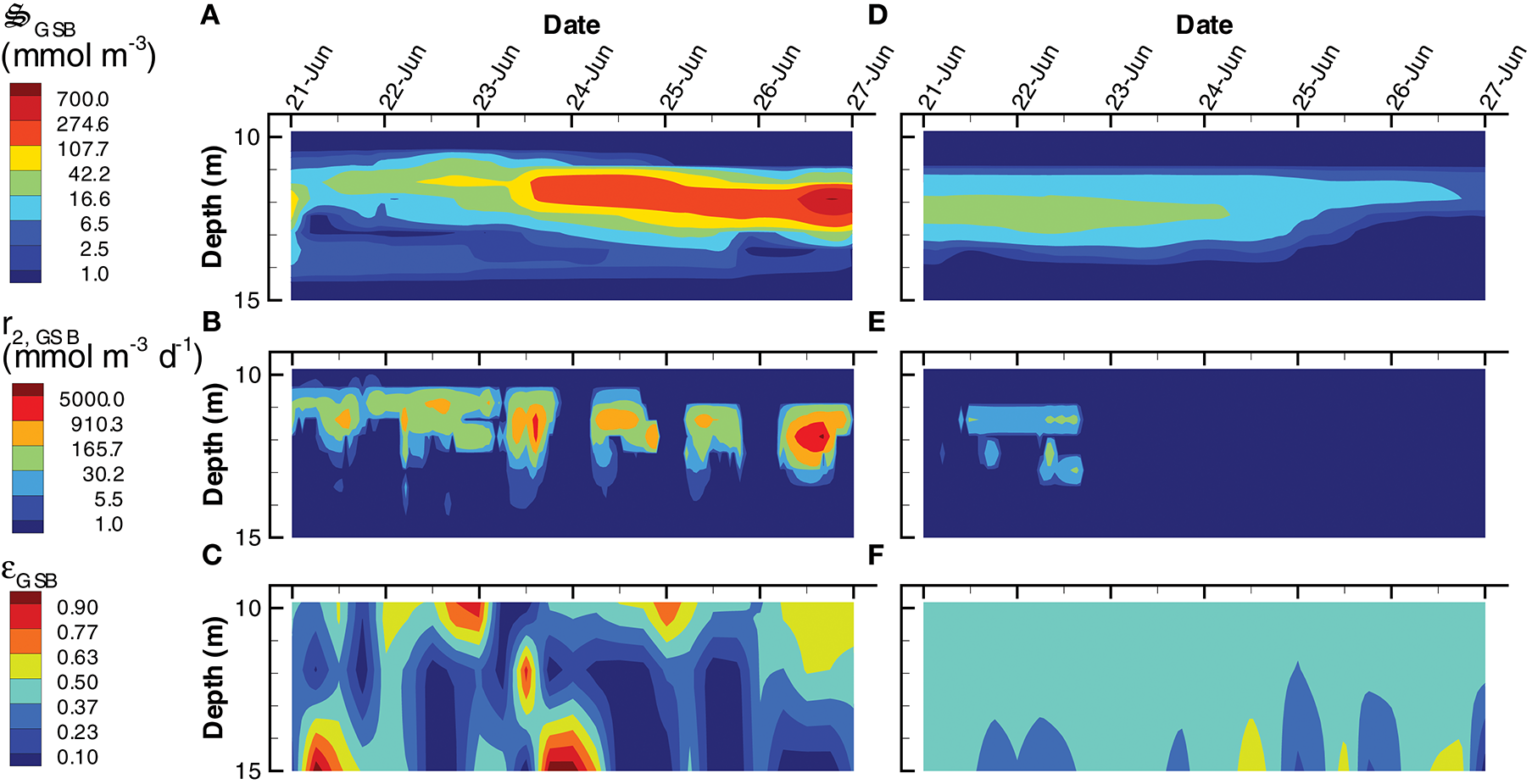
Contour plots of green sulfur bacteria concentration, (A,D), rate of the biosynthesis reaction, r2, GSB(B,E) and the growth efficiency optimal control variable, εGSB(C,F) for the SIO (A–C) and LIO (D–F) simulations. Note, variables are only plotted for 10 m to 15 m where the GSB are active.
Figure 10
Contour plots of photoheterotroph concentration, (A,D), rate of the carbon fixation reaction, r1, PH(B,E) and the growth efficiency optimal control variable, εPH(C,F) for the SIO (A–C) and LIO (D–F) simulations. Note, contours for εPH were selected to emphasize εPH values near zero.
Bacterial densities are similar in the two simulations (Figures S4a,d), but there is significantly higher growth rate by bacteria in the LIO simulation between 4 and 10 m (Figures S4b,e). Both simulations allocate almost all of to detrital carbon decomposition, r2, Bac, below 13 m (Figures S5c,f), but the SIO simulation also allocates biomass to detrital carbon decomposition sporadically throughout the water column to produce CL (Figure S4c). The anaerobic, sulfate reducing bacteria function similarly as bacteria, but operate in the anaerobic portion of the water column (Figures S6, S7). Like bacteria (Bac), the sulfate reducing bacteria (SRB) allocate biomass to detrital carbon decomposition, r2, SRB, below 13 m in both SIO and LIO simulations (Figures S7c,f) and sporadically throughout the water column in the SIO simulation (Figure S7c). Overall, bacteria and SRB function in a complementary mode across the aerobic and anaerobic portions of the water column. Similar to phytoplankton, the control variables for both and show more rapid (bang-bang) control in the SIO compared to the LIO simulation (Figures S5, S7). The third bacterial group, sulfide oxidizing bacteria, , are largely unimportant in either of the 6 day simulations.
Another significant difference between the SIO and LIO simulations is a greater importance of predation, , in the SIO solution (Figure 11). Because predation is abstracted in the MEP model, it represents all predation mechanisms, including protists, predatory bacteria, viruses, and cannibalism. In addition to dissipating chemical potential stored as biomass, predation serves a more important task of recycling nutrients from biomass that are allocated to metabolic functions that are not needed under prevailing conditions. The SIO and LIO simulations show that the concentration of is more than 4 times higher in SIO than LIO solutions, and increases over time under the SIO objective. The primary prey items in the SIO solution are (i.e., cannibalism), and (Figures 11B–D), while only predation is of significance in the LIO solution (Figure 11G). Closer inspection of Figures 11B,C reveals that predation occurs predominately at night, which is a result of temporal changes in the partitioning control variables, Ωi, Gz, rather than prey concentration (not shown). High concentration of is found below 10 m, but growth of grazers actually occurs between 4 and 7 m, which indicates the high concentration below 10 m is due to sinking and accumulation. Accumulation of biomass in the deep, anaerobic, portion of the water column becomes food for anaerobic predators, , which are important in both SIO and LIO simulations, but are slightly more active in the LIO simulation (Figure S8).
Figure 11
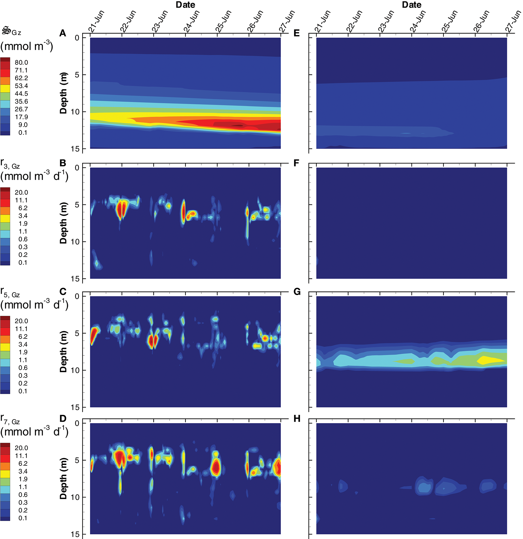
Contour plots of grazer concentration, (A,E) and rates of predation on, grazers, r3, Gz(B,F), bacteria, r5, Gz(C,G), and photoheterotrophs, r7, Gz(D,H) for the SIO (A–D) and LIO (D–H) simulations.
An interesting result that derives from the focus on dissipating energy potentials rather than on growing organisms is the importance of chemotrophs on dissipating electromagnetic potential. For instance, aerobic organoheterotrophic bacteria, , are well understood as dissipaters of chemical potential, as they typically respire significant amounts of organic carbon (i.e., εBac < 0.5). In both the SIO and LIO simulations, however, far more free energy is dissipated by passive light absorption than it is by respiration (Figure 12), although the difference is more striking in the SIO simulation (Figure 12A vs. Figure 12B). Some prokaryotes in nature harness this abundant light energy via expression of proteorhodopsin (Béjà et al., 2000), which is perhaps more widespread than currently appreciated (Dubinsky et al., 2017).
Figure 12
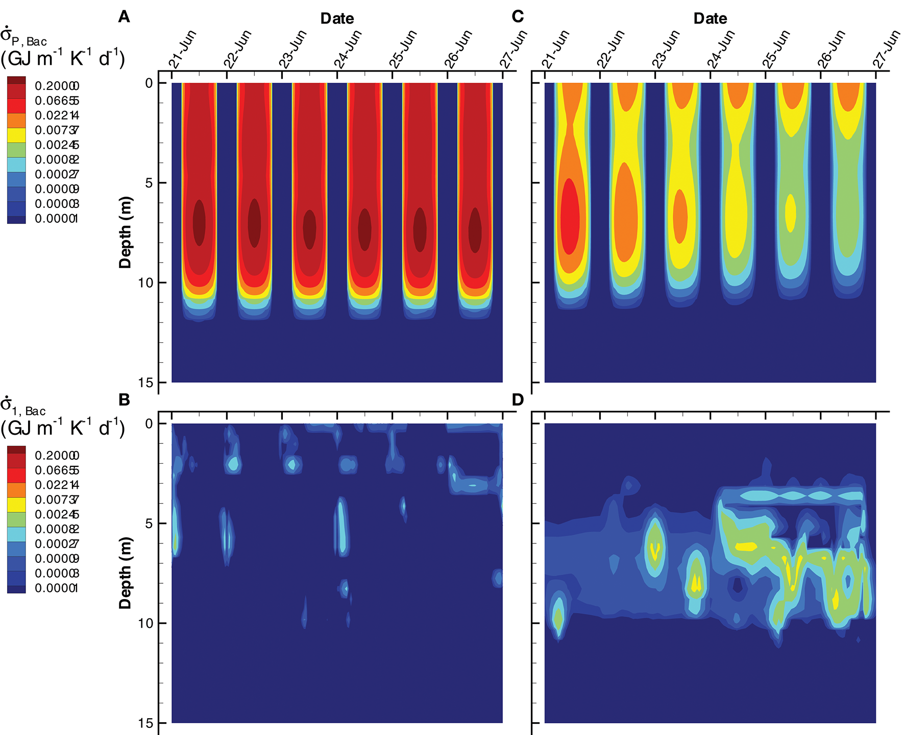
Contour plots of entropy production by bacteria associated with light absorption by bacterial biomass, (A,C) and growth of bacteria, r1, Bac, on organic carbon, , Equation (S94) (B,D) for the SIO (A,B) and LIO (C,D) simulations.
Discussion
The two primary objectives of this study were to demonstrate that (1) a model based on free energy dissipation can reasonably describe microbial community organization and function with relatively few parameters and (2) that microbial systems operate collectively over characteristic timescales that are likely longer than what common wisdom would suggest. The secondary objectives were to demonstrate how the model can be used in systems with spatial dimensions and to extend the approach to include phototrophs. While improvements could be made with explicit data assimilation (Edwards et al., 2015), the MEP model did a reasonable job at simulating biogeochemistry in Siders Pond with few adjustable parameters, and the better fit of the long interval optimization (LIO) simulation to 6 out of 9 observations indicates that the microbial community has evolved to function over time scales that are longer than 0.25 days (Table 3). The MEP optimization approach removed approximately 89 parameters that would have had to be tuned if a conventional model had been used (Ward et al., 2010). Perhaps the most useful aspect is that MEP provides a different perspective to view biology (Skene, 2017). For the Siders Pond model, the perspective focused our attention on how microbial functional activity changes with the length of the entropy integration interval, △t.
Temporal strategies, such as circadian clocks (Wolf and Arkin, 2003), anticipatory control (Mitchell et al., 2009; Katz and Springer, 2016), energy and resource storage (Schulz et al., 1999; Grover, 2011), and dormancy (Lewis, 2010) are hallmarks of biology, yet they are often not given much consideration when theory and models are developed for understanding biogeochemistry, even though temporal strategies have also been observed in microbial communities (Ottesen et al., 2014). Here our model results indicate that different organizational timescales can dramatically impact biogeochemistry and how microbial communities function. For instance, the SIO simulation does not invest resources in phytoplankton growth, because over the short 0.25 day optimization, water dissipates more electromagnetic potential than a small increase in phytoplankton biomass over the short interval. Instead, the SIO solution allocates resources to growth of green sulfur bacteria (GSB) and photoheterotrophs (PH) deeper in the water column to dissipate light not adsorbed by water in the surface. The SIO solution also places more resources on decomposing refractory carbon, but also on respiring the liberated labile carbon. Grazing rates, especially under aerobic conditions, are higher in the SIO simulations as well. These types of resource allocations in the SIO solution appear more consistent with R* or resource-ratio theory (Tilman, 1982) and r-selection (Pianka, 1970; Fierer et al., 2007); that is, emphasis on fast growth. On the contrary, the LIO solution appears more similar to K-selection where resources are invested for longer term outcomes. These differences are also evident in the control variables. In the SIO simulations, the control variables show rapid bang-bang control fluctuations as resources vary (Figure 8D), while the LIO solution produces more gradual changes in control variables (Figure 8I). A microbial community that implements temporal strategies should outcompete a community that lacks temporal strategies, because long-term strategies result in greater acquisition and utilization of food resources under non steady-state conditions than short-term strategies (Cole et al., 2015), which is evident by the 71% greater entropy production over the 6 day simulations using LIO versus SIO (36.5 GJ K−1 vs. 21.3 GJ K−1).
One of the main questions that arise in applying MEP is what is the appropriate timescale over which biology organizes? That is, in the current implementation of the model, what is an appropriate value for △t used in the optimal control problem? In this study two values were explored, 0.25 days for the SIO and 3 days for the LIO. These choices were based on the observation time scale, where 0.25 day is “short” compared to 1 day, and 3 days is “long” in comparison to 1 day. Our results indicate that the SIO solution did not match observations or expectations as well as the LIO solution (Table 3). Comparing MEP model output to observations for differing values of △t is one means to explore this fundamental property of ecosystems. But is a 3 d optimization window sufficient? It seems the appropriate MEP time scales do not depend on just the characteristic time scales of organisms, because our study on periodically forced methanotroph communities showed that the communities were well adapted to 20 day cyclic inputs of energy, even though the characteristic turnover time of bacteria is closer to hours (Vallino et al., 2014; Fernandez-Gonzalez et al., 2016). We know that terrestrial systems function on long timescales, at least on the order of the four seasons, but their time scales are likely much longer given that individual trees can live hundreds of years, and forest succession takes longer than that (Odum, 1969; Finegan, 1984). At this time, we do not have an answer to the question regarding an appropriate optimization time scale for microbial communities, but it is likely related to the time scales over which biological predictions, acquired by evolution, can be reliably made, such as the sun will return tomorrow, or winter is coming. Predicting the future has obvious evolutionary advantages, but it also results in greater dissipation of free energy and entropy production, as evident by the higher entropy produced by the LIO solution. We believe that determining the temporal scales over which microbial communities operate will be important for developing predictive biogeochemistry models, but space scales are also import.
Strategies that coordinate function over space also lead to greater free energy dissipation (Vallino, 2011). Some examples of such coordination include quorum sensing (Goo et al., 2012; Hmelo, 2017) and associated quorum policing (Whiteley et al., 2017), long-range metabolic signaling (Liu et al., 2015), stigmergy (Gloag et al., 2013), horizontal gene transfer (Treangen and Rocha, 2011), cables and nanowires (Reguera et al., 2005; Schauer et al., 2014), cross-feeding (Estrela et al., 2012; Rakoff-Nahoum et al., 2016), chemotaxis (Stocker and Seymour, 2012), vertical migration (Inoue and Iseri, 2012) and other types infochemical exchange (Moran, 2015). Our original intent was to compare local versus global MEP optimization, but global optimization in the Siders Pond model did not produce biologically relevant results due to the speed at which electromagnetic potential is dissipated abiotically. Because water and sediments rapidly absorb light, any water column of sufficient depth will dissipate all incoming radiation as entropy regardless of the presence of organisms, so an infinite number of solutions exist that all produce the same global entropy production. However, maximizing local entropy production at discrete depths, as was conducted in this study, does select for a unique solution, which our results show is biologically relevant. Our previous study with purely chemical reactions showed that global entropy production results in greater chemical potential destruction (Vallino, 2011). This study indicates that if abiotic processes can destroy an energy potential faster than biotic ones, then local MEP optimization will be the preferred solution. Global maximization of entropy production is more likely to be found in systems where energy potentials are stable with respect to abiotic decay, such as chemical potentials. However, it seems possible that both local and global optimization could be operating simultaneously in systems given that both light and chemical potentials often exist, so further studies are needed.
Other areas that could improve the MEP modeling approach are as follows. Our metabolic network (Figure 1) was largely based on prior knowledge about Siders Pond biogeochemistry, but condensing genome-scale models may also be a means to construct more realistic whole community metabolic networks from genomic surveys (Hanson et al., 2014; Hanemaaijer et al., 2015), and exometabolomics could be used to identify metabolite nodes in the distributed metabolic network that are widely exchanged between functional groups (Klitgord and Segre, 2010; Baran et al., 2015; Fiore et al., 2015; Ponomarova and Patil, 2015). Also, our current approach relies on non-linear optimal control to locate MEP solutions, but this is a computationally intensive problem, and falls under the class of problems known as control of partial differential equations (Coron, 2007). Building on expertise from that field could reduce computation requirements, especially for problems involving two or three spatial dimensions, but it might be possible to avoid the formal optimization problem altogether. One possibility would be to use Darwinian inspired trait-based modeling approaches (Follows et al., 2007; Coles et al., 2017), which is how biology actually solves the MEP problem. On the other hand, MEP could be useful for developing trait models that improve entropy production over time and space, such as traits that include resource storage, time delays (i.e., dormancy), migration across fronts and boundaries to acquire resources, clocks and oscillators, distribution and packaging of metabolic function, predation, remineralization, and other regulatory motifs (Wolf and Arkin, 2003). By placing emphasis on the mechanisms of how energy potentials are destroyed over time and space, rather than on the peculiarities of how organisms grow and survive, can lead to new insights that can improve our understanding of biogeochemistry and model predictions thereof.
Conclusions
Our results demonstrate that models based on MEP can reasonably simulate how microbial communities organize and function in Siders Pond over time and space while using a minimum of adjustable parameters. The improved qualitative and quantitative agreement between model predictions and observations using long (3 day, LIO) versus short (0.25 day, SIO) interval optimization supports the hypothesis that biological systems maximize entropy production over long time scales. The modeling presented here extends the MEP approach to include an explicit spatial dimension, and new metabolic reactions were introduced to model phototrophs and entropy production associated with the destruction of electromagnetic potential. By considering the dissipation of both chemical and electromagnetic potentials, the MEP model shows that heterotrophs, such as bacteria, dissipate far more free energy in the photic zone by passive light absorption than by chemical respiration. Short interval optimization results in higher grazing rates and turnover of organic carbon, as well as rapid (bang-bang) changes in the reaction control variables, while long interval optimization supports higher phytoplankton growth and standing stocks near the surface of the pond. We also found that maximization of local entropy production, as opposed to global entropy production, must be used for energy potentials that are quickly dissipated by abiotic processes, such as light absorption by water and particles. Taken together, results validate our general conjecture that biological systems evolve and organize to maximize entropy production over the greatest possible spatial and temporal scales, while abiotic processes maximize instantaneous and local entropy production.
Statements
Author contributions
Both JV and JH contributed equally to project concepts and design, and both conducted the 24 h sampling of Siders Pond. Preliminary results from metatranscriptomics and metagenomics from JH were used to improve development of the metabolic network. JV developed the model and wrote first draft of the manuscript with editing and inputs during the process from JH. Both authors contributed to manuscript revision, read and approved the submitted version.
Funding
Primary funding for this project was from NSF GG grant EAR-1451356 to JV and JH, with additional support from Gordon and Betty Moore Foundation grant GBMF 3297. JV also received support from NSF Grants OCE-1637630 and OCE-1558710 and Simons Foundation grant 549941. The NSF Center for Dark Energy Biosphere Investigations (C-DEBI; OCE-0939564) also supported the participation of JH. This is C-DEBI contribution number 441.
Acknowledgments
We thank Petra Byl for assistance in field work preparation and sampling of Siders Pond, as well as insightful conversations about the project. We also thank Jane Tucker for dissolved inorganic carbon analyses, Suzanne Thomas for hydrogen sulfide analyses, Sam Kelsey for dissolved organic carbon analyses, Kate Morkeski for sulfate, phosphate and particulate organic carbon analyses, and Rich McHorney, Leslie Murphy, Emily Reddington, and Gretta Serres for assistance with Siders Pond sampling logistics. We also thank the Semester in Environmental Science Program at MBL for use of their Hydrolab and Jon Boat used for sampling, and a special thank you to Tom Gregg who allowed us to access Siders Pond through his property as well as for providing logistical support.
Conflict of interest
The authors declare that the research was conducted in the absence of any commercial or financial relationships that could be construed as a potential conflict of interest.
Supplementary material
The Supplementary Material for this article can be found online at: https://www.frontiersin.org/articles/10.3389/fenvs.2018.00100/full#supplementary-material
References
1
AlbertyR. A. (2003). Thermodynamics of Biochemical Reactions. Hoboken, NJ: Wiley and Sons.
2
AlgarC. K.VallinoJ. J. (2014). Predicting microbial nitrate reduction pathways in coastal sediments. Aquat. Microb. Ecol.71, 223–238. 10.3354/ame01678
3
BaranR.BrodieE. L.Mayberry-LewisJ.HummelE.Da RochaU. N.ChakrabortyR.et al. (2015). Exometabolite niche partitioning among sympatric soil bacteria. Nat. Commun.6:8289. 10.1038/ncomms9289
4
BattleyE. H.PutnamR. L.Boerio-GoatesJ. (1997). Heat capacity measurements from 10 to 300 K and derived thermodynamic functions of lyophilized cells of Saccharomyces cerevisiae including the absolute entropy and the entropy of formation at 298.15 K. Thermochim. Acta298, 37–46. 10.1016/S0040-6031(97)00108-1
5
BéjàO.AravindL.KooninE. V.SuzukiM. T.HaddA.NguyenL. P.et al. (2000). Bacterial rhodopsin: evidence for a new type of phototrophy in the sea. Science289, 1902–1906. 10.1126/science.289.5486.1902
6
BlumenfeldL. A. (1981). Problems of Biological Physics.Berlin: Springer-Verlag.
7
BrockT. D. (1981). Calculating solar radiation for ecological studies. Ecol. Model.14, 1–19. 10.1016/0304-3800(81)90011-9
8
CandauY. (2003). On the exergy of radiation. Solar Energy75, 241–247. 10.1016/j.solener.2003.07.012
9
CaracoN. (1986). Phosphorus, Iron, and Carbon Cycling in a Salt Stratified Coastal Pond. Ph.D. thesis, Boston University.
10
CaracoN.PuccoonA. H. (1986). The measurement of bacterial chlorophyll and algalchlorophyll a in natural waters. Limnol. Oceanogr.31, 889–893. 10.4319/lo.1986.31.4.0889
11
CaracoN.TamseA.BoutrosO.ValielaI. (1987). Nutrient limitation of phytoplankton growth in brackish coastal ponds. Can. J. Fish. Aquat. Sci.44, 473–476. 10.1139/f87-056
12
ChapmanE. J.ChildersD. L.VallinoJ. J. (2016). How the Second Law of Thermodynamics has informed ecosystem ecology through its history. BioScience66, 27–39. 10.1093/biosci/biv166
13
ColeJ. A.KohlerL.HedhliJ.Luthey-SchultenZ. (2015). Spatially-resolved metabolic cooperativity within dense bacterial colonies. BMC Syst. Biol.9:15. 10.1186/s12918-015-0155-1
14
ColesV. J.StukelM. R.BrooksM. T.BurdA.CrumpB. C.MoranM. A.et al. (2017). Ocean biogeochemistry modeled with emergent trait-based genomics. Science358, 1149–1154. 10.1126/science.aan5712
15
CoronJ.-M. (2007). Control and Nonlinearity.Providence, RI: American Mathematical Society.
16
DewarR. (2003). Information theory explanation of the fluctuation theorem, maximum entropy production and self-organized criticality in non-equilibrium stationary states. J. Phys. A Math. Gen.36, 631–641. 10.1088/0305-4470/36/3/303
17
DewarR.LineweaverC.NivenR.Regenauer-LiebK. (2014a). Beyond the Second Law: an overview, in Beyond the Second Law, eds DewarR.C.LineweaverC. H.NivenR. K.Regenauer-LiebK. (Berlin; Heidelberg: Springer), 3–27.
18
DewarR. C.LineweaverC. H.NivenR. K.Regenauer-LiebK. (eds) (2014b). Beyond the Second Law: Entropy Production and Non-Equilibrium Systems. Berlin: Springer-Verlag.
19
DubinskyV.HaberM.BurgsdorfI.SauravK.LehahnY.MalikA.et al. (2017). Metagenomic analysis reveals unusually high incidence of proteorhodopsin genes in the ultraoligotrophic Eastern Mediterranean Sea. Environ. Microbiol.19, 1077–1090. 10.1111/1462-2920.13624
20
EdwardsC. A.MooreA. M.HoteitI.CornuelleB. D. (2015). Regional ocean data assimilation. Ann. Rev. Mar. Sci.7, 21–42. 10.1146/annurev-marine-010814-015821
21
EstrelaS.TrisosC. H.BrownS. P. (2012). From metabolism to ecology: cross-feeding interactions shape the balance between polymicrobial conflict and mutualism. Am. Nat.180, 566–576. 10.1086/667887
22
FashamM. J. R.DucklowH. W.McKelvieS. M. (1990). A nitrogen-based model of plankton dynamics in the ocean mixed layer. J. Mar. Res.48, 591–639. 10.1357/002224090784984678
23
FernandezA.HuangS.SestonS.XingJ.HickeyR.CriddleC.et al. (1999). How stable is stable? Function versus community composition. Appl. Environ. Microbiol.65, 3697–3704.
24
Fernandez-GonzalezN.HuberJ. A.VallinoJ. J. (2016). Microbial communities are well adapted to disturbances in energy input. mSystems1:e00117–16. 10.1128/mSystems.00117-16
25
FiererN.BradfordM. A.JacksonR. B. (2007). Toward an ecological classification of soil bacteria. Ecology88, 1354–1364. 10.1890/05-1839
26
FineganB. (1984). Forest succession. Nature312, 109–114. 10.1038/312109a0
27
FioreC. L.LongneckerK.Kido SouleM. C.KujawinskiE. B. (2015). Release of ecologically relevant metabolites by the cyanobacterium Synechococcus elongatus CCMP 1631. Environ. Microbiol.17, 3949–3963. 10.1111/1462-2920.12899
28
FitzpatrickJ. J. (2009). Assessing skill of estuarine and coastal eutrophication models for water quality managers. J. Mar. Syst.76, 195–211. 10.1016/j.jmarsys.2008.05.018
29
FollowsM. J.DutkiewiczS.GrantS.ChisholmS. W. (2007). Emergent biogeography of microbial communities in a model ocean. Science315, 1843–1846. 10.1126/science.1138544
30
FriedrichsM. A. M.DusenberryJ. A.AndersonL. A.ArmstrongR. A.ChaiF.ChristianJ. R.et al. (2007). Assessment of skill and portability in regional marine biogeochemical models: role of multiple planktonic groups. J. Geophys. Res.112:C08001. 10.1029/2006JC003852
31
Gilboa-GarberN. (1971). Direct spectrophotometric determination of inorganic sulfide in biological materials and in other complex mixtures. Anal. Biochem.43, 129–133. 10.1016/0003-2697(71)90116-3
32
GloagE. S.JavedM. A.WangH.GeeM. L.WadeS. A.TurnbullL.et al. (2013). Stigmergy: a key driver of self-organization in bacterial biofilms. Commun. Integr. Biol.6:e27331. 10.4161/cib.27331
33
GoldenfeldN.WoeseC. (2011). Life is physics: evolution as a collective phenomenon far from equilibrium. Annu. Rev. Cond. Matt. Phys.2, 375–399. 10.1146/annurev-conmatphys-062910-140509
34
GooE.MajerczykC. D.AnJ. H.ChandlerJ. R.SeoY. S.HamH.et al. (2012). Bacterial quorum sensing, cooperativity, and anticipation of stationary-phase stress. Proc. Natl. Acad. Sci. U.S.A.109, 19775–19780. 10.1073/pnas.1218092109
35
GroverJ. P. (2011). Resource storage and competition with spatial and temporal variation in resource availability. Am. Nat.178, E124–E148. 10.1086/662163
36
HallamS. J.McCutcheonJ. P. (2015). Microbes don't play solitaire: how cooperation trumps isolation in the microbial world. Environ. Microbiol. Rep.7, 26–28. 10.1111/1758-2229.12248
37
HanemaaijerM.RölingW. F.OlivierB. G.KhandelwalR. A.TeusinkB.BruggemanF. J. (2015). Systems modeling approaches for microbial community studies: from metagenomics to inference of the community structure. Front. Microbiol.6:213. 10.3389/fmicb.2015.00213
38
HansonN. W.KonwarK. M.HawleyA. K.AltmanT.KarpP. D.HallamS. J. (2014). Metabolic pathways for the whole community. BMC Genomics15:619. 10.1186/1471-2164-15-619
39
HmeloL. R. (2017). Quorum sensing in marine microbial environments. Ann. Rev. Mar. Sci.9, 257–281. 10.1146/annurev-marine-010816-060656
40
InoueT.IseriY. (2012). Diel vertical migration and nutrient transport of the dinoflagellate Peridinium bipes F. occultatum in a thermally stratified reservoir. Water Sci. Technol.66, 1212–1219. 10.2166/wst.2012.302
41
JudsonO. P. (2017). The energy expansions of evolution. Nat. Ecol. Evol.1:0138. 10.1038/s41559-017-0138
42
KatzY.SpringerM. (2016). Probabilistic adaptation in changing microbial environments. Peer J.4:e2716. 10.7717/peerj.2716
43
KleidonA.LorenzR. D. (2005). Non-equilibrium Thermodynamics and the Production of Entropy. Berlin: Springer-Verlag.
44
KleidonA.MalhiY.CoxP. M. (2010). Maximum entropy production in environmental and ecological systems. Philos. Trans. R. Soc. B Biol. Sci.365, 1297–1302. 10.1098/rstb.2010.0018
45
KlitgordN.SegrèD. (2010). Environments that induce synthetic microbial ecosystems. PLoS Comput. Biol.6:e1001002. 1–17. 10.1371/journal.pcbi.1001002
46
KonopkaA.LindemannS.FredricksonJ. (2015). Dynamics in microbial communities: unraveling mechanisms to identify principles. ISME J.9, 1488–1495. 10.1038/ismej.2014.251
47
La RoweD. E.DaleA. W.AmendJ. P.Van CappellenP. (2012). Thermodynamic limitations on microbially catalyzed reaction rates. Geochim. Cosmochim. Acta90, 96–109. 10.1016/j.gca.2012.05.011
48
Le QuereC.HarrisonS. P.Colin PrenticeI.BuitenhuisE. T.AumontO.BoppL.et al. (2005). Ecosystem dynamics based on plankton functional types for global ocean biogeochemistry models. Glob. Chang. Biol.11, 2016–2040. 10.1111/j.1365-2486.2005.1004.x
49
LewisK. (2010). Persister cells. Annu. Rev. Microbiol.64, 357–372. 10.1146/annurev.micro.112408.134306
50
LiuJ.PrindleA.HumphriesJ.Gabalda-SagarraM.AsallyM.LeeD. Y.et al. (2015). Metabolic co-dependence gives rise to collective oscillations within biofilms. Nature523, 550–554. 10.1038/nature14660
51
LoceyK. J.LennonJ. T. (2016). Scaling laws predict global microbial diversity. Philos. Trans. R. Soc. B Biol. Sci.113, 5970–5975. 10.1073/pnas.1521291113
52
LorenzR. (2003). Full steam ahead-probably. Science299, 837–838. 10.1126/science.1081280
53
LotkaA. J. (1922). Contribution to the energetics of evolution. Philos. Trans. R. Soc. B Biol. Sci.8, 147–151. 10.1073/pnas.8.6.147
54
LoucaS.DoebeliM. (2016). Transient dynamics of competitive exclusion in microbial communities. Environ. Microbiol.18, 1863–1874. 10.1111/1462-2920.13058
55
MacedoM. F.DuarteP. (2006). Phytoplankton production modelling in three marine ecosystems–static versus dynamic approach. Ecol. Modell.190, 299–316. 10.1016/j.ecolmodel.2005.05.012
56
MarinoN. A. C.SrivastavaD. S.FarjallaV. F. (2016). Predator kairomones change food web structure and function, regardless of cues from consumed prey. Oikos125, 1017–1026. 10.1111/oik.02664
57
MartyushevL. M.SeleznevV. D. (2006). Maximum entropy production principle in physics, chemistry and biology. Phys. Rep.426, 1–45. 10.1016/j.physrep.2005.12.001
58
MitchellA.RomanoG. H.GroismanB.YonaA.DekelE.KupiecM.et al. (2009). Adaptive prediction of environmental changes by microorganisms. Nature460, 220–224. 10.1038/nature08112
59
MoranM. A. (2015). The global ocean microbiome. Science350:aac8455. 10.1126/science.aac8455
60
MorrisonP. (1964). A thermodynamic characterization of self-reproduction. Rev. Mod. Phys.36, 517–524. 10.1103/RevModPhys.36.517
61
MurphyJ.RileyJ. P. (1962). A modified single solution method for the determination of phosphate in natural waters. Anal. Chim. Acta27, 31–36. 10.1016/S0003-2670(00)88444-5
62
NeedhamD. M.FuhrmanJ. A. (2016). Pronounced daily succession of phytoplankton, archaea and bacteria following a spring bloom. Nat. Microbiol.1:16005. 10.1038/nmicrobiol.2016.5
63
OdumE. P. (1969). The strategy of ecosystem development. Science164, 262–270.
64
OttesenE. A.YoungC. R.GiffordS. M.EppleyJ. M.MarinR.SchusterS. C.et al. (2014). Multispecies diel transcriptional oscillations in open ocean heterotrophic bacterial assemblages. Science345, 207–212. 10.1126/science.1252476
65
PasternakZ.Ben SassonT.CohenY.SegevE.JurkevitchE. (2015). A new comparative-genomics approach for defining phenotype-specific indicators reveals specific genetic markers in predatory bacteria. PLOS ONE10:e0142933. 10.1371/journal.pone.0142933
66
PiankaE. R. (1970). R-Selection and K-Selection. Am. Nat.104, 592–597. 10.1086/282697
67
PonomarovaO.PatilK. R. (2015). Metabolic interactions in microbial communities: untangling the Gordian knot. Curr. Opin. Microbiol.27, 37–44. 10.1016/j.mib.2015.06.014
68
Rakoff-NahoumS.FosterK. R.ComstockL. E. (2016). The evolution of cooperation within the gut microbiota. Nature533, 255–259. 10.1038/nature17626
69
ReedD. C.AlgarC. K.HuberJ. A.DickG. J. (2014). Gene-centric approach to integrating environmental genomics and biogeochemical models. Proc. Natl. Acad. Sci. U.S.A.111, 1879–1884. 10.1073/pnas.1313713111
70
RegueraG.McCarthyK. D.MehtaT.NicollJ. S.TuominenM. T.LovleyD. R. (2005). Extracellular electron transfer via microbial nanowires. Nature435, 1098–1101. 10.1038/nature03661
71
RileyG. A. (1946). Factors controlling phytoplankton population on Georges Bank. J. Mar. Res.6, 54–73.
72
SathyendranathS.StuartV.NairA.OkaK.NakaneT.BoumanH.et al. (2009). Carbon-to-chlorophyll ratio and growth rate of phytoplankton in the sea. Mar. Ecol. Prog. Ser.383, 73–84. 10.3354/meps07998
73
SchartauM.WallheadP.HemmingsJ.LöptienU.KriestI.KrishnaS.et al. (2017). Reviews and syntheses: parameter identification in marine planktonic ecosystem modelling. Biogeosciences14, 1647–1701. 10.5194/bg-14-1647-2017
74
SchauerR.Risgaard-PetersenN.KjeldsenK. U.Tataru BjergJ. J. BJørgensenB.SchrammA.et al. (2014). Succession of cable bacteria and electric currents in marine sediment. ISME J. 8, 1314−1322. 10.1038/ismej.2013.239
75
SchulzH. N.BrinkhoffT.FerdelmanT. G.MarinéM. H.TeskeA.JørgensenB. B. (1999). Dense populations of a giant sulfur bacterium in Namibian shelf sediments. Science284, 493–495. 10.1126/science.284.5413.493
76
SkeneK. (2015). Life's a gas: a thermodynamic theory of biological evolution. Entropy17, 5522–5548. 10.3390/e17085522
77
SkeneK. R. (2017). Thermodynamics, ecology and evolutionary biology: a bridge over troubled water or common ground?Acta Oecologica85, 116–125. 10.1016/j.actao.2017.10.010
78
SoginM. L.MorrisonH. G.HuberJ. A.WelchD. M.HuseS. M.NealP. R.et al. (2006). Microbial diversity in the deep sea and the underexplored “rare biosphere”. Proc. Natl. Acad. Sci. U.S.A.103, 12115–12120. 10.1073/pnas.0605127103
79
StockerR.SeymourJ. R. (2012). Ecology and physics of bacterial chemotaxis in the ocean. Microbiol. Mol. Biol. Rev.76, 792–812. 10.1128/MMBR.00029-12
80
TilmanD. (1982). Resource Competition and Community Structure.Princeton, NJ: Princetown University Press.
81
TreangenT. J.RochaE. P. C. (2011). Horizontal transfer, not duplication, drives the expansion of protein families in prokaryotes. PLoS Genet.7:e1001284. 10.1371/journal.pgen.1001284
82
VallinoJ. J. (2000). Improving marine ecosystem models: use of data assimilation and mesocosm experiments. J. Mar. Res.58, 117–164. 10.1357/002224000321511223
83
VallinoJ. J. (2003). Modeling microbial consortiums as distributed metabolic networks. Biol. Bull.204, 174–179. 10.2307/1543554
84
VallinoJ. J. (2010). Ecosystem biogeochemistry considered as a distributed metabolic network ordered by maximum entropy production. Philos. Trans. R. Soc. B Biol. Sci.365, 1417–1427. 10.1098/rstb.2009.0272
85
VallinoJ. J. (2011). Differences and implications in biogeochemistry from maximizing entropy production locally versus globally. Earth Syst. Dynam.2, 69–85. 10.5194/esd-2-69-2011
86
VallinoJ. J.AlgarC. K. (2016). The thermodynamics of marine biogeochemical cycles: lotka revisited. Ann. Rev. Mar. Sci.8, 333–3s56. 10.1146/annurev-marine-010814-015843
87
VallinoJ. J.AlgarC. K.GonzálezN. F.HuberJ. A. (2014). Use of receding horizon optimal control to solve MaxEP-based biogeochemistry problems, in Beyond the Second Law-Entropy Production and Non-Equilibrium Systems, eds DewarR. C.LineweaverC. H.NivenR. K.Regenauer-LiebK. (Berlin; Heidelberg: Springer), 337–359.
88
WardB. A.FriedrichsM. A. M.AndersonT. R.OschliesA. (2010). Parameter optimisation techniques and the problem of underdetermination in marine biogeochemical models. J. Mar. Syst.81, 34–43. 10.1016/j.jmarsys.2009.12.005
89
WhiteleyM.DiggleS. P.GreenbergE. P. (2017). Progress in and promise of bacterial quorum sensing research. Nature551:313. 10.1038/nature24624
90
WolfD. M.ArkinA. P. (2003). Motifs, modules and games in bacteria. Curr. Opin. Microbiol.6, 125–134. 10.1016/S1369-5274(03)00033-X
91
WordenA. Z.FollowsM. J.GiovannoniS. J.WilkenS.ZimmermanA. E.KeelingP. J. (2015). Rethinking the marine carbon cycle: factoring in the multifarious lifestyles of microbes. Science347:1257594. 10.1126/science.1257594
Summary
Keywords
maximum entropy production, microbial biogeochemistry, metabolic networks, phototrophy, community function, meromictic
Citation
Vallino JJ and Huber JA (2018) Using Maximum Entropy Production to Describe Microbial Biogeochemistry Over Time and Space in a Meromictic Pond. Front. Environ. Sci. 6:100. doi: 10.3389/fenvs.2018.00100
Received
07 February 2018
Accepted
23 August 2018
Published
01 October 2018
Volume
6 - 2018
Edited by
Anke Marianne Herrmann, Swedish University of Agricultural Sciences, Sweden
Reviewed by
Mustafa Yucel, Middle East Technical University, Turkey; John Senko, University of Akron, United States
Updates
Copyright
© 2018 Vallino and Huber.
This is an open-access article distributed under the terms of the Creative Commons Attribution License (CC BY). The use, distribution or reproduction in other forums is permitted, provided the original author(s) and the copyright owner(s) are credited and that the original publication in this journal is cited, in accordance with accepted academic practice. No use, distribution or reproduction is permitted which does not comply with these terms.
*Correspondence: Joseph J. Vallino jvallino@mbl.edu
This article was submitted to Microbiological Chemistry and Geomicrobiology, a section of the journal Frontiers in Environmental Science
Disclaimer
All claims expressed in this article are solely those of the authors and do not necessarily represent those of their affiliated organizations, or those of the publisher, the editors and the reviewers. Any product that may be evaluated in this article or claim that may be made by its manufacturer is not guaranteed or endorsed by the publisher.