Assessing Change-Points in Surface Air Temperature Over Alaska

Introduction

Climate scientists are concerned with identifying low frequency variability in regional as well as global climatic conditions. They are also interested in attributing the causes of climate change relative to internal climate variability, and the ways by which governments can mitigate the effects of climate change. The seriousness of these pursuits can be understood by the extensive series of Intergovernmental Panel on Climate Change (IPCC) Assessments.

Detection of variability in the climate system represents one of the toughest challenges. It is only recently that near term climate projection experiments have been carried out focusing on internal climatic variations (Meehl et al., 2011, 2013; Dai et al., 2015). The Pacific Decadal Oscillation (PDO) is an index that tracks dominant variability in the North Pacific with phase shifts developing on decadal time scales (Mantua et al., 1997). Dai et al. (2015) showed that the PDO is also associated with large temperature anomalies over both ocean and land. Other indices that have been associated with temperature anomalies in the North Pacific include Pacific North American pattern (PNA) (Liu et al., 2017), Arctic Oscillation (AO) (Thompson and Wallace, 1998), and others.

Time series analyses of historical data can address the structure of low frequency variability and the detection of potential shifts in the climatic conditions. These shifts are called “change-points” in statistical literature and “structural break-points” in econometrics. Applications of change-point methods for the study of climate change and global warming have been considered in the literature (Gay-Garcia et al., 2009; Dupuis et al., 2015). It is often the case that the presence of one or more shifts or change-points in climatic data collected over a time period remains unknown until they are detected through proper statistical methods (Beaulieu et al., 2012).

Some of the methods that have been implemented for characterizing trends in Alaskan temperatures include: general circulation models (GCMs) (Fyfe et al., 2013; Bennett and Walsh, 2015), cluster analysis (Bieniek et al., 2012), simple linear fit (Wendler and Shulski, 2009; Wendler et al., 2012), stochastic trend (López-de-Lacalle, 2012), and long memory and seasonality (Gil-Alana, 2012). While these methods have merits, they also lack the ability to accommodate complex non-stationary trends in the temperature series. This is particularly the case with simple linear trend models. For example, López-de-Lacalle (2012) states that a linear fit does not appear to be plausible since the long-term pattern is more step-like than approximately linear. Step-like linear trend models were considered by Stevenson et al. (2012) and Bone et al. (2010), where data series were split into two or more sub-parts by choosing cut-off times as per the changing cycles of a proxy variable such as the PDO. This approach amounts to fitting a step-like model where the authors apriori fix both the number of cut-off points as well as their locations over time. Instead, change-point methods are better suited to fit step-like models where the change-point model itself selects both the number of steps as well as their locations, thereby removing the arbitrariness in choosing them apriori.

Clearly, existing literature on Alaskan climate lacks proper scientific way of identifying shifts in its temperature series. The same is true regarding the series on PDO. Noting that change-point methods are better suited for identifying unknown shifts in time series, the focus of this article is to apply recently developed change-point methods to data on surface air temperatures (SATs) of southern Alaska and northern North Pacific regions as well as in PDO series so that shifts in these series are identified in a scientifically valid manner.

Methods

Description of Datasets and Variables

Several types of datasets have been considered in this article. These include: temperature anomalies, PDO, 500 mb geopotential height field anomalies, and sea level pressure (SLP) anomalies. In this section we begin by providing the sources of each of these datasets and describe other relevant aspects including the variables considered in the analysis.

Regarding data on temperature anomalies, seven stations from the state of Alaska (elevations between 12 and 475 ft) were investigated (Figure 1) in this analysis. Daily and monthly surface air temperature measurements were obtained from Weather Source (http://weathersource.com/). Weather Source obtains data from National Oceanic and Atmospheric Administration (NOAA), National Climatic Data Center (NCDC), and the National Weather Service (NWS). The seven stations are: AB–Auke Bay, AC–Annex Creek, JIA–Juneau International Airport, FIA–Fairbanks International Airport, UES–University Experimental Station, KSA–King Salmon Airport, and HA–Homer Airport. The selection of stations was based on geographic location, climate division they represent (Bieniek et al., 2012), continuity of the data, and years for which data was available (see Table 1 for complete information). We made every effort to utilize as much of data as possible for any given station without compromising on the quality and continuity. Weather Source utilizes multiple methods and data sources to clean the data and replace invalid values with “best estimates.” Even so, we needed to shorten the data length for some stations due to missing observations. For example, there were instances where data was missing continuously for several months in a year. In such cases we have removed the entire year from our analysis. At the same time, we have ensured that data was continuously available for every single year reported at any given station. There were only few occasional months when data was missing. On such occasional months, the missing observations were filled by simulations based on mean and variance of five values before and after each missing observation. In order to make clear that missing observations were rare, we have included the % of missing months for all seven locations in Table 1.We shall now move on to describe the temperature variables that were part of the analysis in this article. Most studies that analyze temperature trends of the Alaska region use data on mean temperatures (Hartmann and Wendler, 2005; Wendler and Shulski, 2009; Bone et al., 2010; Bieniek et al., 2012, 2014; López-de-Lacalle, 2012; Stevenson et al., 2012; Wendler et al., 2012). However, it is important to consider changes in temperature conditions that are further away from the mean as they generally have greater impact on humans and ecosystems (Bennett and Walsh, 2015). With this in mind, we evaluate changes in monthly maxima, means, and minima. Nine temperature variables Max_Grt (highest value over a month of daily maxima), Mean_Grt (highest value over a month of daily means), Min_Grt (highest value over a month of daily minima), Max_Avg (average value over a month of daily maxima), Mean_Avg (average value over a month of daily means), Min_Avg (average value over a month of daily minima), Max_Lst (lowest value over a month of daily maxima), Mean_Lst (lowest value over a month of daily means), and Min_Lst (lowest value over a month of daily minima) for each month for which data is available are considered in the study.

FIGURE 1

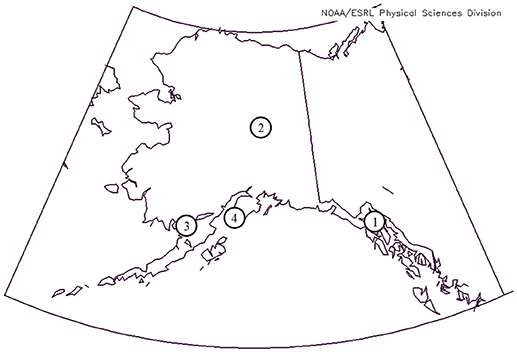
Figure 1. Spatial distribution of all seven stations; stations located too close to each other are identified by the same number on the map (see the list below for complete information about each station).

Station information:

TABLE 1

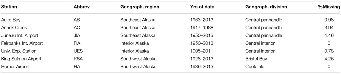
Table 1. Locations of temperature measuring stations, their abbreviations, the geographical region each station represents, years of data included in the study for each station, the climate division each station belongs, and the % of months for which observations were missing.

Trends in temperatures for the Alaska region are carried out in the past on a seasonal basis (Stafford et al., 2000; López-de-Lacalle, 2012) defined as: winter = Dec–Feb, spring = Mar–May, summer = Jun–Aug, fall = Sep–Nov. For any variable, seasonal data was computed from the monthly data by taking the average of the three monthly observations of the season.

When strong correlations are present among pairs of variables, there is scope for deleting some of the variables due to redundancy. Upon carrying out a thorough correlation analysis among all the nine variables (details not presented), we found that Mean_Grt, Mean_Avg and Mean_Lst were redundant. Hence, these three variables were dropped from the study altogether and the rest of the study consists of only the remaining six variables.

Regarding PDO, data on standardized PDO indices for each month of a given year for the years 1900–2013 were obtained from http://research.jisao.washington.edu/pdo/PDO.latest. These observations were utilized to compute PDO data for seasonal maximum, average, and minimum for every year. Apart from the PDO, other time series that may be related to southern Alaska and North Pacific climate variability include: geopotential height field (Overland et al., 2015), sea level pressure (SLP) (Johnstone and Mantua, 2014), Madden-Julian Oscillations (MJO) (Zhou et al., 2011; Oliver, 2014), Aleutian low pressure (Wendler et al., 2012; Johnstone and Mantua, 2014), greenhouse gas concentrations (Holland and Bitz, 2003), and volcanic aerosol loading and solar radiation (Overpeck et al., 1997). Among these, we shall consider in this article only the geopotential height field anomalies and SLP anomalies. Accordingly, the images for 500 mb geopotential height field anomalies and SLP anomalies were taken from the website http://www.esrl.noaa.gov/psd/ maintained by NOAA/ESRL Physical Sciences Division, Boulder, Colorado. The images themselves are based on Kalnay et al. (1996), a reanalysis project that produces various atmospheric fields. While complete details of data characteristics may be found in this article, we note here that spatially, the field data are based upon 2.5° latitude × 2.5° longitude grid. Even though we didn't consider here, other levels for geopotential field maps may also be considered such as 200, 700, or 1,000 mb.

Change-Point Detection

Our objective is to study trends in each of the six temperature variables and four seasons through change-point analysis. We shall also implement change-point analysis for identifying shifts in PDO data. Here we would like to mention that other indices such as PNA and AO could also be included in this study for identifying shifts. However, we mainly considered the PDO since data for this index is available from 1900 onwards whereas data for both PNA and AO starts from the year 1950 only. Briefly, change-point analysis is a statistical methodology developed for detecting and identifying unknown locations of one or more time points at which a given data over time might have changed its statistical properties. Thus, given a time series data one might propose that there exist m number of change-points occurring at unknown locations. The change-points could occur in either the mean or the variance of the data. The goal of change-point analysis is to estimate the number of change-points m and their locations. There has been substantial interest in recent literature for identifying multiple change-points—some of the prominent methods are: binary segmentation (BS) (Cho and Fryzlewicz, 2015), optimal partitioning (OP) (Jackson et al., 2005), pruned exact linear time (PELT) (Killick et al., 2012, 2014), Bayesian (Li and Lund, 2015), and minimum description length (MDL) (Davis et al., 2006; Li and Lund, 2012). For a more complete discussion and review of multiple change-point methods, one may see Jandhyala et al. (2013). In this article, we adapt the PELT method for detecting and identifying multiple change-points. There are many key advantages of the PELT method. First, it is an exact method and under mild conditions it has a computational cost that is linear in the number of data points. Killick et al. (2012) have shown that that PELT is better than OP. Also, PELT is more accurate than binary segmentation and faster than other exact search methods (Wambui et al., 2015). Furthermore, Wambui et al. (2015) investigated the power properties of PELT in relation to the size of change and also location of change-points. They found that the power of PELT increased with the size of change and that for a given size, the power remained the same for any location of change-points. Also, Corneli et al. (2017) compared PELT against triclustering approach of Guigourès et al. (2018) and found PELT to be superior for identifying multiple change-points in dynamical networks. The complete steps of the PELT algorithm are presented in Appendix 1.

Before we go ahead and implement PELT, we wish to state that PELT can be sensitive to the arbitrariness in choosing two of its parameters – (i) the nature of penalty function, and (ii) the gap between successive change-points. The authors (Killick et al., 2014) state that there is no objective way to pick an appropriate penalty function for PELT. So, one must fine tune the penalty function by trial and error before arriving at the chosen one. For example, for identifying changes in mean, the penalty functions we considered in our trial and error ranged between 10logn to 60logn. In the case of identifying changes in variance, the penalty functions ranged between 2logn to 3logn. The choice for the gap between two successive change-points mostly depends upon the particular application. For both temperature and PDO series, we chose this gap to be a minimum of 10 years. This particular choice avoids spurious and excessive number of change-points and at the same time does not unduly lower the number of identified changes.

While implementing PELT, we aim to identify multiple change-points in both the mean and variance of any given temperature variable. Upon detecting changes in both mean and variance, diagnostic checks have been performed on residuals and concluded that almost all variables including those that represented extremes followed the normal distribution quite well and that there were no serial correlations in the data series. Earlier, López-de-Lacalle (2012) also found both of these assumptions to be valid while studying Alaskan temperature changes among seasons through a time varying model.

The PELT method does not provide p-values or confidence intervals associated with the identified change-points. Hence, we first applied likelihood ratio change detection test (Csörgő and Horváth, 1997) and computed p-values for change-points identified by PELT. If the change in mean was significant (p-value < 0.05), a 95% (approx.) confidence interval (Fotopoulos et al., 2010) was calculated for the change-point. Methods of applying change detection test and computing the distribution of change-point estimate are both presented in Appendix 2. Here we need to note that the change-points identified may be either “artificial” shifts or “natural” shifts caused by climatic changes. Artificial shifts in data may occur due to changes in instrumentation, or other changes in the observation process. Such changes in data observation process are usually documented in the data collection process and one should be able to associate an identified shift as an artificial shift through a thorough understanding of the data.

Upon identifying the change-points, the percent of total variation (%Variation) explained by the change-point model is of interest. This is computed from %Variation = (SSM/SST) × 100, where SSM is the variation due to the change-point model and SST is the total sum of squares. One would also be interested in exploring whether there is spatial and temporal consistency in the detected number of change-points. This can be assessed by performing a contingency analysis on the number of detected change-points among various stations and seasons. However, in trying to ensure that the number of change-points was not too small in any given cell, we combined the seven stations into three geographical regions—central panhandle (AB, AC, JIA); central interior (FIA, UES); Bristol Bay and Cook Inlet (KSA, HA). Among seasons, it was sufficient to combine summer and fall into one group. Thus, we performed contingency table analysis among three regions and the three seasons.

Apart from the proposed change-point methodology, one must be open to other ways of modeling regime shifts such as modeling the data as a red noise process. The residuals under change-point methodology resemble a white noise process, where the observations have mean zero, finite variance and are serially uncorrelated (Overland et al., 2006). The observations in a red noise process also have mean zero and finite variance but are serially correlated. As noted by Overland et al. (2006), any time series with shifts in mean may also be modeled by a red noise process. For purposes of illustration, we pursue here only the autoregressive process of order one (AR(1)) as a red noise model and that too for variables with shifts in PDO data only. It then becomes a matter of whether the change-point model with white noise errors or the AR(1) model with red noise errors is better for modeling shifts in PDO variables. Here, we employ the widely used Akaike Information Criterion (AIC) (Akaike, 1974) for choosing the preferred model. Values of AIC are computed using AIC = −2 log (maximum likelihood) + 2 (# of independent parameters in the model). Upon computing AIC values, one chooses the model with smaller AIC as the preferred model.

Results and Discussion

Throughout the 7 stations, 4 seasons, 6 temperature variables, and PDO, changes were significant predominantly in the mean but not in varince. Overall, PELT identified change in variance only at 5 instances, one each at AB, AC, JIA, KSA, and HA. Among these, only the change in Max_Lst at HA was found to be statistically significant. Thus, throughout this study, we present results for changes in mean only. Table 2 shows results on change-points for PDO. The table consists of change-points identified by PELT, approximate 95% confidence interval (±years) computed only when p-value for a PELT change-point is < 0.05, and the [amount of change in mean]. Among the 7 stations, similar results on change-points for stations JIA, FIA, and KSA are presented in Tables 3A–C, respectively; JIA represents southeastern region, FIA represents interior region, and KSA represents southwestern region. Similar results for the remaining 4 stations AB, AC, UES, and HA are presented in Tables 4A–D. In both Tables 3A–C, Tables 4A–D, we exclude all variables for which PELT did not identify any change-points. In Figure 2 we plot the time series data for all PDO variables in all seasons together with mean level for each data segment as determined by significant change-points. When no significant change-point was found, a single mean level for the entire period is drawn for such variables. Similar depictions of data together with change-points for temperature variables are presented in Figures 3–5, selecting one station from each geographical region: Figure 3 – JIA (southeastern); Figure 4 – FIA (interior); Figure 5 – KSA (southwestern). To save space, we do not include such figures for other stations. Values of SST, SSE, SSM, and %Variation for representative stations of JIA, FIA, and KSA are presented in Table 5. Similar values for stations AB, AC, UES, and HA are presented Table 6. While we carried out the contingency table analysis among the three geographical regions and the three seasons, we do not include the corresponding contingency table to save space. However, we discuss the results of this analysis in the next section. Finally, we present in Table 7 the AIC values for AR(1) and change-point models for any PDO variable with at least one significant change-point (see Table 2, Figure 2).

TABLE 2

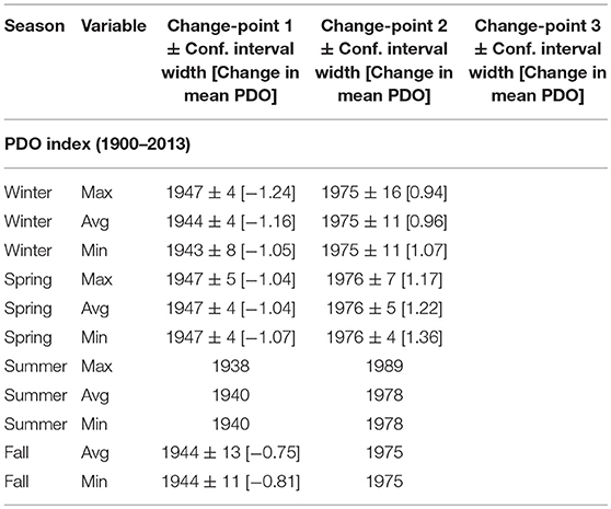
Table 2. Change-points in mean for PDO with: PELT change-point estimate ± width of approximate 95% confidence interval (when change detection test p-value < 0.05) and [amount of change in mean PDO], or only PELT change-point estimate (when change detection test p-value > 0.05).

TABLE 3A

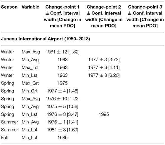
Table 3A. Change-points in mean for station JIA representing southeastern region of Alaska with: PELT change-point estimate ± width of approximate 95% confidence interval (when change detection test p-value < 0.05) and [amount of change in mean in °C], or only PELT change-point estimate (when change detection test p-value > 0.05).

TABLE 3B

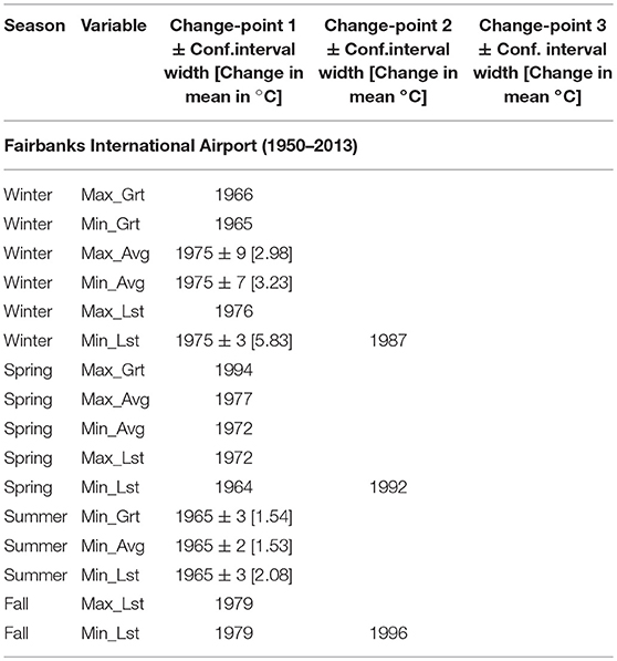
Table 3B. Change-points in mean for station FIA representing interior region of Alaska with: PELT change-point estimate ± width of approximate 95% confidence interval (when change detection test p-value < 0.05) and [amount of change in mean in °C], or only PELT change-point estimate (when change detection test p-value > 0.05).

TABLE 3C

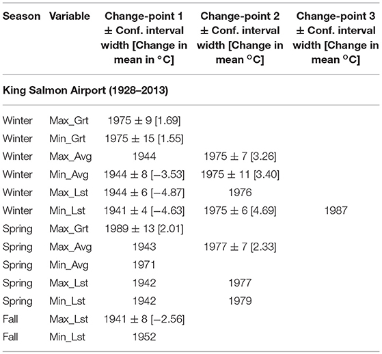
Table 3C. Change-points in mean for station KSA representing southwestern region of Alaska with: PELT change-point estimate ± width of approximate 95% confidence interval (when change detection test p-value < 0.05) and [amount of change in mean in °C], or only PELT change-point estimate (when change detection test p-value > 0.05).

TABLE 4A

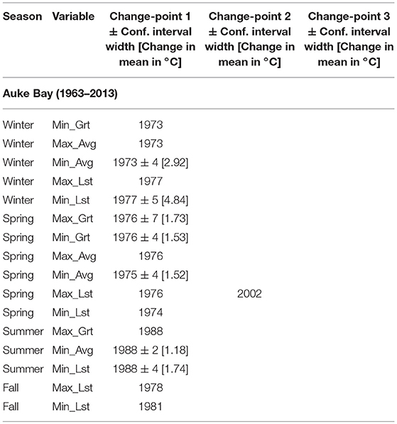
Table 4A. Change-points in mean for station AB of Alaska with: PELT change-point estimate ± width of approximate 95% confidence interval (when change detection test p-value < 0.05) and [amount of change in mean in °C], or only PELT change-point estimate (when change detection test p-value > 0.05).

TABLE 4B

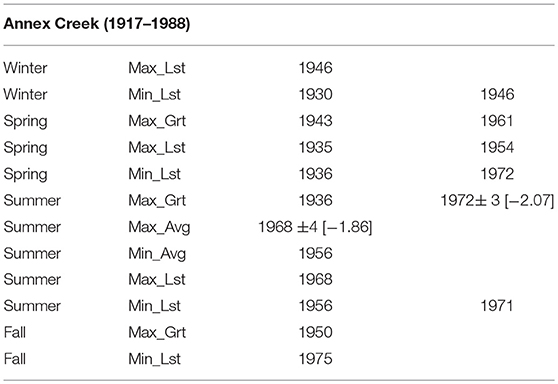
Table 4B. Change-points in mean for station AC of Alaska with: PELT change-point estimate ± width of approximate 95% confidence interval (when change detection test p-value < 0.05) and [amount of change in mean in °C], or only PELT change-point estimate (when change detection test p-value > 0.05).

TABLE 4C

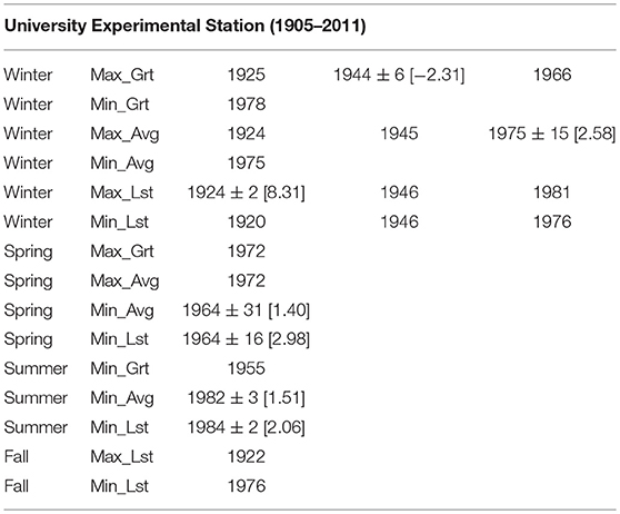
Table 4C. Change-points in mean for station UES of Alaska with: PELT change-point estimate ± width of approximate 95% confidence interval (when change detection test p-value < 0.05) and [amount of change in mean in °C], or only PELT change-point estimate (when change detection test p-value > 0.05).

TABLE 4D

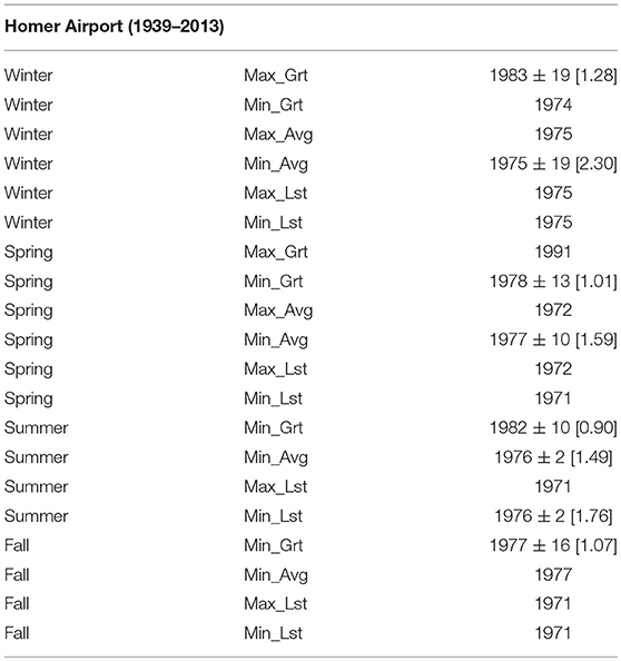
Table 4D. Change-points in mean for station HA of Alaska with: PELT change-point estimate ± width of approximate 95% confidence interval (when change detection test p-value < 0.05) and [amount of change in mean in °C], or only PELT change-point estimate (when change detection test p-value > 0.05).

FIGURE 2

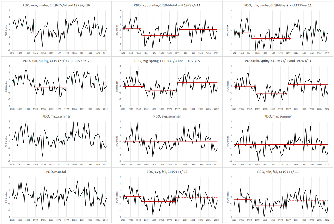
Figure 2. PDO indices for the time-period 1928–2013 for variables maximum, average, and minimum for each of the four seasons together with data means within each segment, where each segment is determined by change-point analysis for PDO indices; solid red lines represent data means within each segment with shifts identified by both the PELT method and the change detection test statistic; dashed red lines indicate data means for segments identified by PELT method but not confirmed by the change detection static when at least one other change is detected by both the PELT method and the change detection statistic.

FIGURE 3

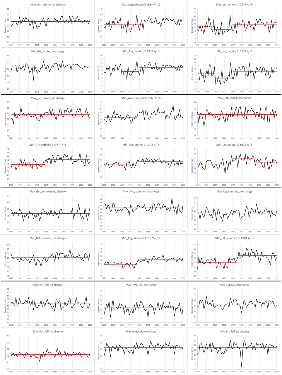
Figure 3. JIA temperature data series for the time-period 1950–2013 for variables Max_Grt, Min_Grt, Max_Avg, Min_Avg, Max_Lst, and Min_Lst for winter (A: Rows 1–2), spring (B: Rows 3–4), summer (C: Rows 5–6), and fall (D: Rows 7–8) together with data means within each segment, where each segment is determined by change-point analysis; solid red lines represent data means within each segment with shifts identified by both the PELT method and the change detection test statistic; dashed red lines indicate data means for segments identified by PELT method but not confirmed by the change detection static when at least one other change is detected by methods.

FIGURE 4

Figure 4. FIA temperature data series for the time-period 1950–2013 for variables Max_Grt, Min_Grt, Max_Avg, Min_Avg, Max_Lst, and Min_Lst for winter (A: Rows 1–2), spring (B: Rows 3–4), summer (C: Rows 5–6), and fall (D: Rows 7–8) together with data means within each segment, where each segment is determined by change-point analysis; solid red lines represent data means within each segment with shifts identified by both the PELT method and the change detection test statistic; dashed red lines indicate data means for segments identified by PELT method but not confirmed by the change detection static when at least one other change is detected by both methods.

FIGURE 5

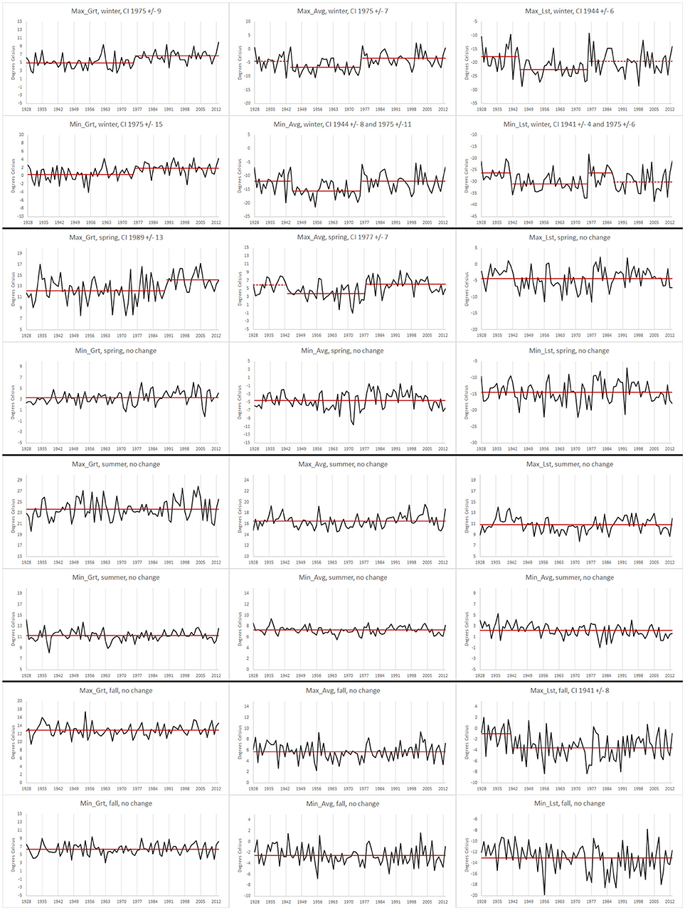
Figure 5. KSA temperature data series for the time-period 1928–2013 for variables Max_Grt, Min_Grt, Max_Avg, Min_Avg, Max_Lst, and Min_Lst for winter (A: Rows 1–2), spring (B: Rows 3–4), summer (C: Rows 5–6), and fall (D: Rows 7–8) together with data means within each segment, where each segment is determined by change-point analysis; solid red lines represent data means within each segment with shifts identified by both the PELT method and the change detection test statistic; dashed red lines indicate data means for segments identified by PELT method but not confirmed by the change detection static when at least one other change is detected by both methods.

TABLE 5

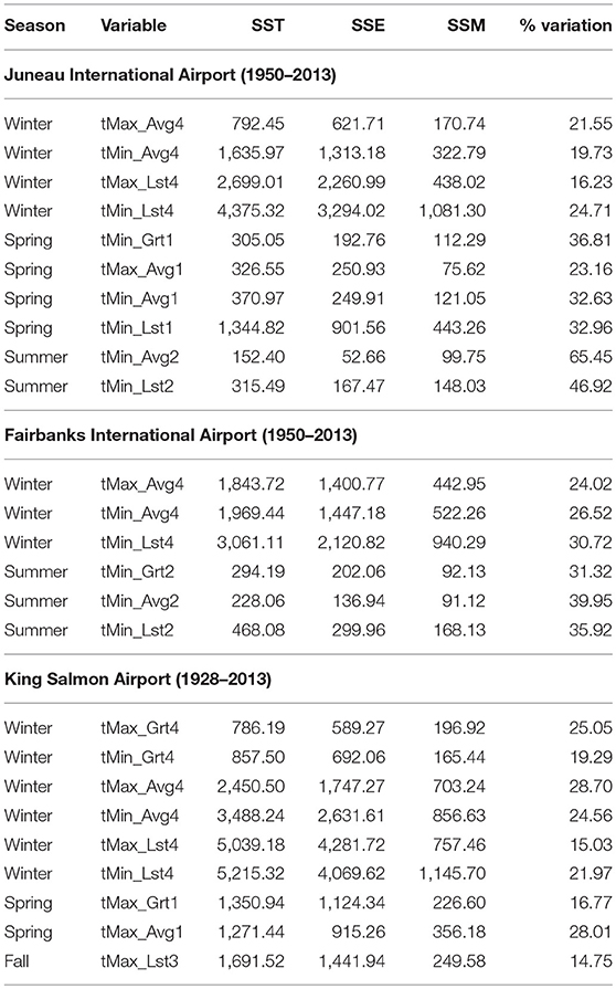
Table 5. Values of total sum of squares (SST), sum of squares of squares due to error (SSE), sum of squares due to model (SSM), and %Variation = (SSM/SST) × 100 for all variables in all seasons with at least one significant change-point at stations JIA (representing southeastern region), FIA (representing interior region), and KSA (representing southwestern region).

TABLE 6

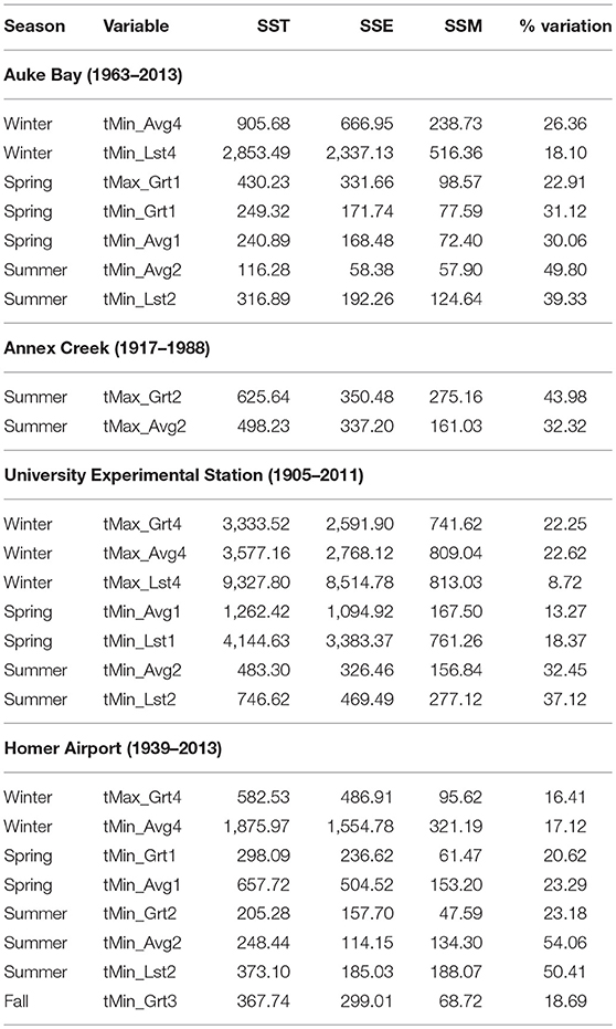
Table 6. Values of total sum of squares (SST), sum of squares of squares due to error (SSE), sum of squares due to model (SSM), and %Variation = (SSM/SST) × 100 for all variables in all seasons with at least one significant change-point at stations AB, AC, UES, and HA of Alaska.

TABLE 7

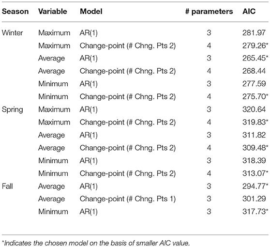
Table 7. Akaike Information Criterion (AIC) values for PDO data for AR (1) model (auto regressive model of order 1) and change-point model with either two or one change-points computed for variables with significant change-point (s) in a given season.

We begin our discussion of results with AIC values in Table 7. Clearly, among eight PDO variables for which AIC has been computed, AIC prefers change-point model for five (winter_Max, winter_Min, spring_Max, spring_Avg, spring_Min), and AR(1) model for three (winter_Avg, fall_Avg, fall_Min). Thus, there is greater preference for change-point model over the red noise AR(1) model. Here, a good understanding of the physical nature of each of these two models is important. For example, the time points at which regime shifts take place are deterministic in a change-point model, whereas they are the result of purely random variations in an AR(1) model. Consequently, in a red noise model such as the AR(1), the times of shifts may not have any specific physical interpretation. However, the times of shifts in a change-point model may often be the result of one or more deterministic causes. A challenge in proposing a change-point model is in identifying the causes that lead to regime shifts in the underlying process.

Next, we discuss values for %Variation presented in Tables 5, 6. The range of values for %Variation for each station are: AB – (18.10, 49.80), AC – (32.32, 42.98), JIA – (16.23, 65.45), FIA – (24.02, 39.95), UES – (8.72, 37.12), KSA – (14.75, 28.70), and HA – (16.41, 54.06). These percent variations explained by their respective models may seem to be on the lower side. This means error variability forms a greater component of the total variability when compared to the model variability. However, when compared relative to their respective degrees of freedom, mean model variability will far exceed mean error variability and one will then note that the model would be statistically significant. Furthermore, López-de-Lacalle (2012) recently evaluated percent variation explained by PDO values for six stations in Alaska including Fairbanks, King Salmon, and Homer. The overall range for percent variation explained by PDO for the six stations considered in López-de-Lacalle (2012) was (2.08, 60.15), a range comparable to what we found here (8.72, 65.45) for seven stations.

The contingency analysis among three regions (central panhandle, central interior, Bristol Bay and Cook Inlet) and three seasons [winter, spring, (summer and fall)] yielded a chi-square statistic value of 2.74. Based upon 4 degrees of freedom for the chi-square statistic, the corresponding p-value was 0.6022. This implies that there is homogeneity among regions and seasons as far as number of change-points is concerned.

For PDO indices (Table 2, Figure 2) changes in maximum, average, and minimum were relatively similar within a given season. There is strong evidence for two changes in all three variables during winter and spring seasons. The first change in winter (a cooling phase) began after 1944 (±4 years) with amount of change in the range −1.24 to −1.05, and the second change (warming phase) began after 1975 (±11 years) with amount ranging from 0.94 to 1.07. The two changes in spring were quite similar to those in winter season (1947 ± 4, amount −1.07 to −1.04; and 1976 ± 5, amount 1.17 to 1.36). During fall season, a change in the mid-1940s (1944 ± 11) occurred in average and minimum variables, while no significant changes were found in any of the variables during summer. Also, changes that apply to all three variables (maximum, average, and minimum) are strong only for winter and spring. Otherwise, they are weakly present during fall and non-existent during summer. If one goes by a presumed approximately 20–30 year cycle of warming and cooling phases for PDO (Mantua et al., 1997; McLean et al., 2009), then one would expect a change to have occurred around the year 2000 (25 years after the change in the mid-1970s). However, no significant change was found around the year 2000 in PDO. Similarly, 25 years prior to the change in the mid-1940s, one might have expected a change around the year 1920. However, despite data being available from 1900, no significant change was found around the year 1920. Thus our analysis is not supportive of a consistent 20–30 year cyclic behavior in PDO. If PDO is an important factor for temperature changes in Alaska, then, temperature changes should also be minimal to non-existent in the 1920s. To see whether this bears out, among the seven stations we have considered in this study, there is sufficient temperature data only at UES (1905–2011) station. At this station, no significant changes were found in and around in 1920s, except for only one variable in winter. Thus, both PDO and UES station seem to show some similarity in the absence of changes in 1920s.

For temperature changes among stations, seasons and variables (see Tables 3A–C, Tables 4A–D, Figures 3–5), there were many instances where likelihood ratio test showed no significance to changes identified by PELT. For example, from Table 4B it is clear that PELT identified two change-points at AC twice: Min_Lst – 1930 and 1946 during winter; and Max_Lst – 1935 and 1954 during spring. However, all of these changes were not statistically significant as per the change detection test (p-values not shown in Table 4B were within 0.236 to 0.907). Overall, from Tables 3A–C, Tables 4A–D, Figures 3–5, it is clear that most of the significant changes in temperatures occurred either in mid-1940s or in mid-1970s.

Temperature changes in mid-1940s are relevant only for stations AC, UES, and KSA (need sufficient data prior to mid-1940s). Among these, no significant change occurred at AC (Table 4B) in the mid-1940s while one change occurred at UES (Table 4C) in Max_Grt during winter (1944 ± 6, amount of change: −2.31°C). Most number of changes were at KSA (Table 3C, Figure 5) with winter having three changes (Min_Avg, Max_Lst, Min_Lst; amount of change: −4.87°C to −3.53°C) followed by one change in fall (Max_Lst; amount of change: −2.56°C). Overall, the average amount of change in the mid-1940s is −3.58°C, and the cooling occurred mostly at KSA (southwestern region) station leaving out both AC (southeastern region) and UES (central region) stations with little change.

As for temperature changes in the mid-1970s, all seven stations are relevant (all have sufficient data). We shall first prepare a tally of number of times temperature changes occurred in the mid-1970s separately for stations, seasons and variables. In doing so, we consider a change to have occurred in the mid-1970s if the estimated time of change (when significant) was within the range 1972–1978. From Tables 3A–C, Tables 4A–D, Figures 3–5, it follows that temperatures changed in the mid-1970s for a total of 30 times (including one cooling instance at AC). The tally of these 30 changes at each station, season and variable, and the corresponding average amounts of change [average change °C] are as follows: stations: AB−5 [2.51], AC−1 [2.07], JIA−8 [2.90], FIA−3 [4.01], UES−1 [2.58], KSA−6 [2.82], HA−6 [1.54]; seasons: winter−15 [3.55], spring−10 [1.74], summer−4 [1.68], fall−1 [1.07]; variables: Max_Grt−3 [1.83], Min_Grt−5 [1.33], Max_Avg−5 [2.47], Min_Avg−10 [2.32], Max_Lst−1 [4.11], Min_Lst−6 [4.47]. From the above tally, it is clear that there is considerable variability in the number of changes as well as in the average amount of change among stations, seasons and variables. It is more appealing to view the changes at stations from geographical region point of view—the corresponding number of changes and average amounts are: southeastern−14 [2.70]; interior−4 [3.65]; southwestern−12 [2.18]. Clearly, southeastern and southwestern regions dominate the number of changes in the mid-1970s (total of 26 changes from 5 stations of southeastern and southwestern regions compared to 4 changes from 2 stations of interior Alaska). However, the highest average amount of change (3.65°C) occurs in the central region. Seasonally, winter and spring account for most of the changes in the mid-1970s (total of 25 changes) while summer and fall together consist of only 5 changes. This is consistent with the warming phase of PDO in the mid-1970s, where significant changes were found predominantly in winter and spring only. Moreover, the highest seasonal average amount of change (3.55°C) occurs during winter.

It is pertinent to view our results against earlier studies. Stafford et al. (2000) analyzed temperature data from 1949 to 1998 for 25 stations representing throughout Alaska. Their analysis based on mean temperatures showed annual and seasonal mean temperatures increased all across the state, and highest increase (2.2°C) occurred in winter in the interior of Alaska. This is in agreement with our findings except that in our case, the average amounts are somewhat higher (winter 3.55°C; interior 3.65°C). The higher amount of change in our case can be justified due to the fact that our analysis includes various extremes, whereas the analysis of Stafford et al. (2000) is based on mean temperatures. Applying best linear fit to data from 1906 to 2006 from Fairbanks, Wendler and Shulski (2009) found that changes in temperature were not uniform over the seasons in a year, just as the results of this study also vary over the seasons. Their seasonal data analysis showed that mean temperature increased during winter, spring, and summer, while it decreased slightly during fall. We found significant increases during winter and summer seasons at FIA and no significant changes during spring and fall. Wendler and Shulski (2009) attributed the increase in winter temperatures to increased advection due to a more intense Aluetian low. Hartmann and Wendler (2005) analyzed Alaskan temperature for the period 1951–2001 to study shift in 1976; they found mean temperatures increased by as much as 3.1°C after the year 1976. The overall increase from the 30 changes in the mid-1970s of our study is 3.49°C, which is slightly higher, quite likely due to various extremes in our study, than Hartmann and Wendler (2005).

Since changes in extremes are important, we compare changes in the two extreme variables Max_Grt and Min_Lst. With 6 changes Min_Lst dominates the changes compared to the 3 changes in Max_Grt. Furthermore, the average change in Min_Lst is 4.47°C, whereas in Max_Grt it is 1.83°C. The 4.5°C average for Min_Lst is highest among the averages for all six variables. Bennett and Walsh (2015) also noted that the largest amount of change occurred in the extreme minimum.

In addition to changes in the mid-1970s (1972–1978), there were 6 earlier changes in 1960s (AC summer−1, FIA summer−3, UES spring−2), and 9 changes that occurred in 1980s (AB summer-2, JIA winter−1, JIA summer−1, UES summer−2, KSA spring−1, HA winter−1, HA summer−1). Among the 15 early or late changes, 10 occurred during summer. From Tables 3A–C, Tables 4A–D, it follows that the average amount of change from these 10 early or late summer changes is 1.61°C. Thus, it is not that changes did not occur in summer, but most changes in summer were either early or late compared to the mid-1970s. To our knowledge, this anomaly was not identified earlier in the literature and is worth pursuing further.

Some observations regarding similarities and dissimilarities for changes in the mid-1970s at nearby stations are also noteworthy. Stations AB, AC, and JIA (southeastern region) are in close proximity and yet their changes are all not similar (see Tables 3A, 4A,B and also Figure 3 for JIA). Among differences, temperatures at AB and JIA during winter and spring became warmer after 1976 (±6 years) whereas, at AC, temperatures became cooler during summer after 1969 (±5 years). The most visible common feature among these stations is that no significant changes occurred during fall. Stations FIA and UES (interior Alaska) are also close to one another. While they possess some similarities, there are also differences (see Table 3B and Figure 4 for FIA, and Table 4C for UES). Looking at similarities, no significant changes occurred during fall at both stations. Also, changes at both stations occurred in Max_Avg during winter, and in Min_Avg and Min_Lst during summer. Among differences, while changes at FIA were after 1975 (±8 years) in winter, and after 1965 (±3 years) in summer, changes at UES occurred at variable times during winter and after 1982 (±3 years) during summer. Stations KSA and HA may be considered to be relatively close and there were 6 changes at each of these stations, showing some similarity. However, 5 of the 6 changes at KSA occurred during winter compared to either 1 or 2 changes per season that occurred at HA (see Tables 3C, 4D, also Figure 5 for KSA).

Relationships Between Variables

López-de-Lacalle (2012) noted that changes in PDO had strong relation to Alaskan temperature changes and that the effect was variable across locations and seasons. Even nearby stations showed differences in PDO correlations.

Apart from PDO, other fields that correlate to temperature changes in arctic and Alaskan region include: geopotential height field (Overland et al., 2015), sea level pressure (SLP) (Timlin and Walsh, 2007; Johnstone and Mantua, 2014), Madden-Julian Oscillations (MJO) (Oliver, 2014), and Aleutian low pressure (Wendler et al., 2012). Most weather systems follow the 500 mb pressure level and the corresponding geopotential level for explaining changes in surface air temperature. While Overland et al. (2015) associate geopotential height to Alaskan temperature changes, they also mention other reasons such as: reduced summer albedo due to sea ice and snow cover loss; decrease of total cloudiness in summer and increase in winter; and additional heat generated by newly formed sea-ice free ocean areas. Other recent articles that associate geopotential height with climatic changes include Shulski et al. (2010), Schnetzler and Dierking (2008), Bond and Harrison (2006), Hartmann and Wendler (2005), and Bitz and Battisti (1999). Most recently Johnstone and Mantua (2014) studied interrelationships between Northeast Pacific (includes Alaska region) SLP, sea surface temperature (SST) and adjacent land SAT. Based on linear regression analysis, Johnstone and Mantua (2014) found that the positive trend in SAT is reduced by more than 80% when adjusted for SLP variability. The MJO is a dominant mode of large-scale sub-seasonal tropospheric variability over the tropical Indian and Pacific Oceans (Vecchi and Bond, 2004). Oliver (2014) found that MJO was strongly connected with SAT temperature change at Fairbanks during the period 1946–1966. In close agreement with Oliver (2014), in this article, we found significant change around 1965 during summer at FIA and during spring at UES (see Tables 3B, 4C, also Figure 4 for FIA). Apart from being a driver of PDO, the Aleutian low pressure also accounted for nearly all of the observed SST and SAT warming around the coastal northeast Pacific Arc (Johnstone and Mantua, 2014).

Following the above observations, we construct 500 mb geopotential height composite anomaly maps for southeastern region (stations AB, AC, JIA) for 5 years before change (1974–1978) for winter season (Figure 6A) and the corresponding 5 years after change (1979–1983) map (Figure 6B). We also prepared similar 5 year composite anomaly before and after change maps for SLP (see Figures 6C,D). In both geopotential and SLP cases, one can see substantial differences in before change to after change maps.

FIGURE 6

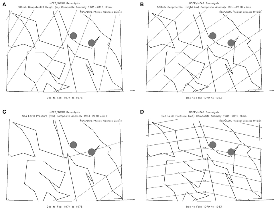
Figure 6. Composite anomaly 500 mb geopotential height for southeastern region of Alaska for (A) Five year before change (1974–1978), and (B) Five year after change (1979–1983); composite anomaly Sea Level Pressure (SLP) measured in millibars (mb) for (C) Five year before change (1974–1978), and (D) Five year after change (1979–1983) for southeastern region of Alaska (consisting of stations AB and JIA marked on left and AC on right) for winter months of December–February.

Next, we explore reasons for significant warming that occurred in Min_Grt and Min_Lst variables during summer of 1965 at FIA station. Even though Oliver (2014) associated MJO with such SAT temperature changes at Fairbanks, we construct 500 mb geopotential height and SLP maps for June-August period at FIA region: Figure 7A has the 5 years before change (1961–1965) composite anomaly 500 mb geopotential height map, and Figure 7B has the corresponding map for 5 years after the change (1966–1970); the corresponding before change and after change composite anomaly maps for SLP are displayed in Figures 7C,D. Here, the before and after change maps are markedly different in both geopotential height and SLP cases. The differences in these before and after change maps are reflective of the temperature changes that might have occurred at surface level around the year 1965 at FIA station.

FIGURE 7

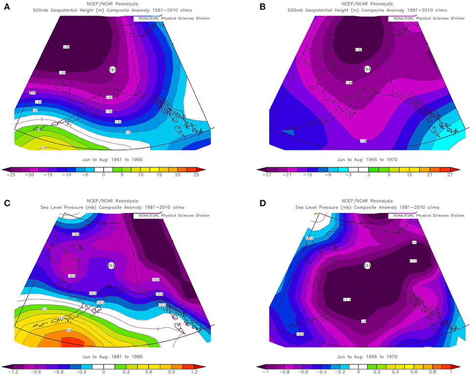
Figure 7. Composite anomaly 500 mb geopotential height for (A) Five year before change (1961–1965), and (B) Five year after change (1966-1970); Composite anomaly Sea Level Pressure (SLP) measured in millibars (mb) for (C) Five year before change (1961–1965), and (D) Five year after change (1966–1970) for summer months June-Aug at FIA station (marked).

Some additional studies have also considered temperature changes in Alaskan region (Overpeck et al., 1997; Holland and Bitz, 2003; ACIA, 2005; Hinzman et al., 2005; Kaufman et al., 2009; Wood and Overland, 2010; Walsh et al., 2011; Koenigk et al., 2015). For example, Wood and Overland (2010) debate reasons for the early twentieth century arctic temperature warming and conclude it was due to internal variability. Overpeck et al. (1997) suggested that before 1920 volcanic aerosol loading and solar radiation were contributors to arctic SAT changes. Subsequent to 1920 increasing greenhouse gas concentrations dominated arctic temperature variability, an observation supported by Holland and Bitz (2003).

An aspect that requires discussion is the differences in temperature changes at nearby stations. For example, stations AB, AC, and JIA are all nearby stations and yet temperature changes in the mid-1970s do not quite match (see Table 4A for AB, Table 4B for AC, and Table 3A and Figure 3 for JIA). This is particularly true of JIA and AC which are separated by a distance of about 30 miles. The cooling in summer at AC and the warming in winter, spring and summer at JIA are quite contrasting. Before exploring any external factors, we first computed correlations for various variables across all seasons for all nearby stations including between AC and JIA (correlations are not shown). The correlations we computed are not uniformly high across all seasons and variables. Specifically, between AC and JIA, we notice that 8 out of 24 correlations (33%) are below 0.50. Thus, it appears that some external factors do indeed seem to alter temperature behaviors at these two close by stations.

What are possible explanations for differences in temperature behaviors at AC and JIA? Geographically, southeastern Alaska is a rugged mountainous terrain and weather conditions can vary considerably within short distances. Moreover, Juneau is on the bank of the Gastineau channel whereas Annex Creek is on the interior bank of the Taku Inlet. Dierking (1998) studied how nearby locations in the area differed substantively in terms of their pressure gradients and maximum wind gusts during the occurrence of Taku wind events. Colman and Dierking (1992) noted that downtown Juneau was located on the fringe of the full force of the wind and hence did not usually record the more severe values.

Conclusions

We have identified changes in temperature series at seven Alaskan weather stations and in PDO series. Most of the changes were during winter and spring in the mid-1940s or in the mid-1970s, in agreement with changes in the PDO. While, there were no significant changes in the mid-1970s during summer, there were early or late changes in summer, an anomaly that has not been identified earlier in climatological studies. Southwestern and southeastern regions of Alaska accounted for most of the changes in the mid-1970s compared to the interior of Alaska. The amount of change was the greatest in Min_Lst.

While this study supports deterministic regime shifts for the northern North Pacific temperature variability due to internal and external forcing, random red-noise processes AR(1) cannot be ruled out as a plausible alternative. The percent variation explained by the change-point models was found to be in the range (8.72, 65.45). This range is comparable with (2.08, 60.15) that López-de-Lacalle (2012) computed between the PDO and Alaskan temperatures. It should be noted that shifts in temperature can have a lasting impact on other important Alaskan and Arctic factors including sea ice, arctic snow cover, atmospheric heat transport, clouds, and others. In this regard this article can perhaps enable climate scientists to study the wider issue of impact on Alaskan climatic factors due to temperature shifts identified here.

Author Contributions

EK, VJ, and SF worked together on developing the ideas, collecting data sources, approaches to statistical analyses, and in carrying out the computations and analyses. JO contributed in writing the introduction by properly contextualizing this study with other relevant climatological studies. All authors worked together in writing the discussion of results and their interpretations.

Funding

The research of JO was supported by Arctic Research Program of the NOAA Climate Prediction Office; PMEL Contribution # 4037.

Conflict of Interest Statement

The authors declare that the research was conducted in the absence of any commercial or financial relationships that could be construed as a potential conflict of interest.

Acknowledgments

The authors are grateful to two referees who have given valuable comments and suggestions on an earlier version of the article. Their suggestions and comments have led to substantial improvements in the paper, both in content and style.

Supplementary Material

The Supplementary Material for this article can be found online at: https://www.frontiersin.org/articles/10.3389/fenvs.2018.00121/full#supplementary-material

References

ACIA (2005). Arctic Climate Impact Assessment-Scientific Report. London: Cambridge University Press.

Akaike, H. (1974). A new look at the statistical model identification. IEEE Trans. Auto. Contr. 19, 716–723. doi: 10.1109/TAC.1974.1100705

CrossRef Full Text | Google Scholar

Beaulieu, C., Chen, J., and Sarmiento, J. (2012). Change-point analysis as a tool to detect abrupt climate variations. Phil. Trans. Roy. Soc. A 370, 1228–1249. doi: 10.1098/rsta.2011.0383

PubMed Abstract | CrossRef Full Text | Google Scholar

Bennett, K. E., and Walsh, J. E. (2015). Spatial and temporal changes in indices of extreme precipitation and temperature for Alaska. Int. J. Climatol. 35, 1434–1452. doi: 10.1002/joc.4067

CrossRef Full Text | Google Scholar

Bieniek, P. A., Bhatt, U. S., Thoman, R. L., Angeloff, H., Partain, J., Papineau, J., et al. (2012). Climate divisions for Alaska based on objective methods. J. Appl. Meteor. Climatol. 51, 1276–1289. doi: 10.1175/JAMC-D-11-0168.1

CrossRef Full Text | Google Scholar

Bieniek, P. A., Walsh, J. E., Thoman, R. L., and Bhatt, U. S. (2014). Using climate divisions to analyze variations and trends in Alaska temperature and precipitation. J. Clim. 27, 2800–2818. doi: 10.1175/JCLI-D-13-00342.1

CrossRef Full Text | Google Scholar

Bitz, C. M., and Battisti, D. S. (1999). Interannual to decadal variability in climate and glacier mass balance in Washington, western Canada and Alaska. J. Clim. 12, 3181–3196

Google Scholar

Bond, N. A., and Harrison, D. E. (2006). ENSO's effect on Alaska during opposite phases of the Arctic Oscillation. Int. J. Climatol. 26, 1821–1841. doi: 10.1002/joc.1339

CrossRef Full Text | Google Scholar

Bone, C., Alessa, L., Kliskey, A., and Altaweel, M. (2010). Influence of statistical methods and reference dates on describing temperature change in Alaska. J. Geophy. Res. 115. doi: 10.1029/2010JD014289

CrossRef Full Text | Google Scholar

Cho, H., and Fryzlewicz, P. (2015). Multiple-change-point detection for high dimensional time series via sparsified binary segmentation. J. Roy. Statist. Soc. B 77, 475–507. doi: 10.1111/rssb.12079

CrossRef Full Text | Google Scholar

Colman, B. R., and Dierking, C. F. (1992). The Taku wind of southeast Alaska: its identification and prediction. Wea. Forecast. 7, 49–64.

Google Scholar

Corneli, M., Latouche, P., and Rossi, F. (2017). Multiple change-points and clustering in dynamic networks. Statist. Comp. 28, 989–1007. doi: 10.1007/s11222-017-9775-1

CrossRef Full Text | Google Scholar

Csörgő, M., and Horváth, L. (1997). Limit Theorems in Change-point Analysis. New York, NY: John Wiley.

Google Scholar

Dai, A., Fyfe, J. C., Xie, S.-P., and Dai, X. (2015). Decadal modulation of global surface temperature by internal climate variability. Nat. Clim. Change 5, 555–560. doi: 10.1038/nclimate2605

CrossRef Full Text | Google Scholar

Davis, R., Lee, T. C. M., and Rodriguez-Yam, G. A. (2006). Structural estimation for non-stationary time series models. J. Amer. Statist. Assoc. 101, 223–239. doi: 10.1198/016214505000000745

CrossRef Full Text | Google Scholar

Dierking, C. F. (1998). Effects of a mountain wave windstorm at the surface. Wea. Forecasting 13, 606–616. doi: 10.1175/1520-0434(1998)013<0606:EOAMWW>2.0

CrossRef Full Text | Google Scholar

Dupuis, D. J., Sun, Y., and Wang, H. J. (2015). Detecting change-points in extremes. Stat. Interface 8, 19–31. doi: 10.4310/SII.2015.v8.n1.a3

CrossRef Full Text | Google Scholar

Fotopoulos, S. B., Jandhyala, V. K., and Khapalova, E. (2010). Exact asymptotic distribution of the change-point mle for change in the mean of Gaussian sequences. Ann. Appl. Stat. 4, 1081–1104. doi: 10.1214/09-AOAS294

CrossRef Full Text | Google Scholar

Fyfe, J. C., von Salzen, K., Gillett, N. P., Arora, V. K., Flato, G. M., and McConnell, J. R. (2013). Variability and trends of air temperature and pressure in the maritime Arctic. Nat. Sci. Repo. 3:2645. doi: 10.1038/srep02645

CrossRef Full Text | Google Scholar

Gay-Garcia, C., Estrada, F., and Sánchez, A. (2009). Global and hemispheric temperatures revisited. Clim. Change 94, 333–349. doi: 10.1007/s10584-008-9524-8

CrossRef Full Text | Google Scholar

Gil-Alana, L. A. (2012). Long memory, seasonality and time trends in the average monthly temperature in Alaska. Theor. Appl. Clomatol. 108, 385–396. doi: 10.1007/s00704-011-0539-0

CrossRef Full Text | Google Scholar

Guigourès, R., Boullé, M., and Rossi, F. (2018). Discovering patterns in time varying graphs: a triclustering approach. Adv. Data Anal. Class. 12, 509–536. doi: 10.1007/s11634-015-0218-6

CrossRef Full Text | Google Scholar

Hartmann, B., and Wendler, G. (2005). On the significance of the 1976 Pacific climate shift in the climatology of Alaska. J Clim. 18, 4824–4839. doi: 10.1175/JCLI3532.1

CrossRef Full Text | Google Scholar

Hinzman, L. D., Bettez, N. D., Bolton, W. R., Chapin, S. F., Dyurgerov, M. B., Fastie, C. L., et al. (2005). Evidence and implications of recent climate change in northern Alaska and other Arctic regions. Clim. Change 72, 251–298. doi: 10.1007/s10584-005-5352-2

CrossRef Full Text | Google Scholar

Holland, M. M., and Bitz, C. M. (2003). Polar amplification of climate change in coupled models. Clim. Dyn. 21, 221–232. doi: 10.1007/s00382-003-0332-6

CrossRef Full Text | Google Scholar

Jackson, B., Sargle, J. D., Barnes, D., Arabhi, S., Alt, A., Gioumousis, P., et al. (2005). An algorithm for optimal partitioning of data on interval. IEEE Signal Process. Lett. 12, 105–108. doi: 10.1109/LSP.2001.838216

CrossRef Full Text | Google Scholar

Jandhyala, V. K., Fotopoulos, S. B., MacNeill, I. B., and Liu, P. (2013). Inference for single and multiple change-points in time series. J. Time Ser. Anal. 34, 423–446. doi: 10.1111/jtsa.12035

CrossRef Full Text | Google Scholar

Johnstone, J. A., and Mantua, N. J. (2014). Atmospheric controls on north east Pacific temperature variability and change, 1900-2012. Proc. Natl. Acad. Sci. 111, 14360–14365. doi: 10.1073/pnas.1318371111

CrossRef Full Text | Google Scholar

Kalnay, E., Kanamitsu, M., Kistler, R., Collins, W., Deaven, D., Gandin, L., et al. (1996). The NCEP/NCAR 40-year reanalysis project. Bull. Am. Meteorol. Soc. 77, 437–471. doi: 10.1175/1520-0477(1996)077<0437:TNYRP>2.0.CO;2

CrossRef Full Text | Google Scholar

Kaufman, D. S., Schneider, D. P., McKay, N. P., Ammann, C. M., Bradley, R. S., Briffa, K. R., et al. (2009). Recent warming reverses long-term arctic cooling. Science 325:1236–1239. doi: 10.1126/science.1173983

PubMed Abstract | CrossRef Full Text | Google Scholar

Killick, R., Eckley, I., and Haynes, K. (2014). Changepoint: An R Package for Changepoint Analysis. R Package Version 1.1.5. Available online at http://CRAN.R-project.org/package=changepoint

Google Scholar

Killick, R., Fearnhead, P., and Eckley, I. A. (2012). Optimal detection of change-points with a linear computational cost. J. Amer. Stat. Assoc. 107, 1590–1598. doi: 10.1080/01621459.2012.737745

CrossRef Full Text | Google Scholar

Koenigk, T., Berg, P., and Döscher, R. (2015). Arctic climate change in an ensemble of regional CORDEX simulations. Polar Res. 34:24603. doi: 10.3402/polar.v34.24603

CrossRef Full Text | Google Scholar

Li, Y., and Lund, R. (2012). Multiple change-point detection via genetic algorithm. J. Clim. 25, 674–686. doi: 10.1175/2011JCLI4055.1

CrossRef Full Text | Google Scholar

Li, Y., and Lund, R. (2015). Multiple changepoint detection using metadata. J. Clim. 28, 4199–4216. doi: 10.1175/JCLI-D-14-00442.1

CrossRef Full Text | Google Scholar

Liu, Z., Tang, Y., Jian, Z., Poulsen, C., Welker, J., and Bowen, G. (2017). Pacific North American circulation pattern links external forcing and Borth American hydroclimatic change over the past millennium. Proc. Nation. Acad. Sci. 114, 3340–3345. doi: 10.1073/pnas.1618201114

CrossRef Full Text | Google Scholar

López-de-Lacalle, J. (2012). Trends in Alaska temperature data. Towards a more realistic approach. Clim. Dyn. 38, 2131–2141. doi: 10.1007/s00382-011-1198-7

CrossRef Full Text | Google Scholar

Mantua, N. J., Hare, S. R., Zhang, Y., Wallace, J. M., and Francis, R. C. (1997). A Pacific interdecadal climate oscillation with impacts on salmon production. Bull. Am. Meteorol. Soc. 78, 1069–1079.

Google Scholar

McLean, J. D., Freitas, C. R., and Carter, R. M. (2009). Influence of the southern oscillation on tropospheric temperature. J. Geophys. Res. 114:D14104. doi: 10.1029/2008JD011637

CrossRef Full Text | Google Scholar

Meehl, G. A., Arblaster, J. M., Fasullo, J. T., Hu, A., and Trenberth, K. E. (2011). Model-based evidence of deep-ocean heat uptake during surface-temperature hiatus periods. Nat. Clim. Change 1, 360–364. doi: 10.1038/nclimate1229

CrossRef Full Text | Google Scholar

Meehl, G. A., Hu, A., Arblaster, J. M., Fasullo, J. T., and Trenberth, K. E. (2013). Externally forced and internally generated decadal climate variability associated with the Interdecadal Pacific Oscillation. J. Clim. 26, 7298–7310. doi: 10.1175/JCLI-D-12-00548.1

CrossRef Full Text | Google Scholar

Oliver, E. C. J. (2014). Multidecadal variations in the modulation of Alaska wintertime air temperature by the Madden-Julian Oscillation. Theor. Appl. Climatol. 121, 1–11. doi: 10.1007/s00704-014-1215-y

CrossRef Full Text | Google Scholar

Overland, J. E., Hanna, E., Hanssen-Bauer, I., Kim, S.-J., Walsh, J. E., Wang, M., et al. (2015). Surface Air Temperature. Arctic Report Card: Update for 2015. Available online at: https://www.arctic.noaa.gov/Report-Card/Report-Card-2015/ArtMID/5037/ArticleID/210/Surface-Air-Temperature

Overland, J. E., Percival, D. B., and Mofjeld, H. O. (2006). Regime shifts and red noise in the North Pacific. Deep-Sea Res. I 53, 582–588. doi: 10.1016/j.dsr.2005.12.011

CrossRef Full Text | Google Scholar

Overpeck, J., Hughen, K., Hardy, D., Bradley, R., Case, R., Douglas, M., et al. (1997). Arctic environmental change of the last four centuries. Science 278, 1251–1256. doi: 10.1126/science.278.5341.1251

CrossRef Full Text | Google Scholar

Schnetzler, A. E., and Dierking, C. F. (2008). Seasonal temperature and precipitation dependencies in southeast Alaska. Natl. Wea. Dig. 32, 93–108. doi: 10.1.1.663.9658

CrossRef Full Text | Google Scholar

Shulski, M., Walsh, J., Stevens, E., and Thoman, R. (2010). Diagnosis of extended cold-season temperature anomalies in Alaska. Mon. Weath. Rev. 138:453–462. doi: 10.1175/2009MWR3039.1

CrossRef Full Text | Google Scholar

Stafford, J. M., Wendler, G., and Curtis, J. (2000). Temperature of Alaska: 50 year trend analysis. Theor. Appl. Climatol. 67, 33–44. doi: 10.1007/s007040070014

CrossRef Full Text | Google Scholar

Stevenson, K., Alessa, L., Altaweel, M., Kliskey, A. D., and Krieger, K. E. (2012). Minding our methods: How choice of time series, reference dates, and statistical approach can influence the representation of temperature change. Environ. Sci. Technol. 46, 7435–7441. doi: 10.1021/es2044008

PubMed Abstract | CrossRef Full Text | Google Scholar

Thompson, D. W. J., and Wallace, J. M. (1998). The Arctic oscillation signature in the wintertime geopotential height and temperature fields. Geophys. Res. Lett. 25, 1297–1300. doi: 10.1029/98GL00950

CrossRef Full Text | Google Scholar

Timlin, M. S., and Walsh, J. E. (2007). Historical and projected distributions of daily temperature and pressure in the arctic. Arctic 60, 389–400.

Google Scholar

Vecchi, G., and Bond, N. (2004). The Madden-Julian Oscillation (MJO) and northern high latitude wintertime surface air temperatures. Geophy. Res. Lett. 31:L04104. doi: 10.1029/2003GL018645

CrossRef Full Text | Google Scholar

Walsh, J. E., Overland, J. E., Groisman, P. Y., and Rudolf, B. (2011). Ongoing climate change in the arctic. Ambio 40, 6–16. doi: 10.1007/s13280-011-0211-z

CrossRef Full Text | Google Scholar

Wambui, G., Waititu, G., and Wanjoya, A. (2015). The power of the pruned exact linear time (PELT) test in multiple change-point detection. Am. J. Th. Appl. Statist. 4, 581–586. doi: 10.11648/j.ajtas.20150406.30

CrossRef Full Text | Google Scholar

Wendler, G., Chen, L., and Moore, B. (2012). The first decade of the new century: a cooling trend for most of Alaska. Open Atmos. Sci. J. 6, 111–116. doi: 10.2174/1874282301206010111

CrossRef Full Text | Google Scholar

Wendler, G., and Shulski, M. (2009). A century of climate change for Fairbanks, Alaska. Arctic 62, 295–300. doi: 10.14430/arctic149

CrossRef Full Text | Google Scholar

Wood, K. R., and Overland, J. E. (2010). Early 20^th century arctic warming in retrospect. Int. J. Climatol. 30, 1269–1279. doi: 10.1002/joc.1973

CrossRef Full Text | Google Scholar

Zhou, Y., Thomson, K., and Lu, Y. (2011). Mapping and understanding the relationship between northern hemisphere winter surface temperature and the Madden-Julian Oscillation. Mon. Wea. Rev. 139, 2439–2445. doi: 10.1175/2011MWR3587.1

CrossRef Full Text | Google Scholar