Robustness and Scalability of Regional Climate Projections Over Europe

1. Introduction

In the IPCC Special Report on Global Warming of 1.5°C (IPCC, 2018), a global warming of 1.5°C above pre-industrial levels is used as a target to understand how this warming will impact society and how drastic climate change mitigation actions are needed. At the current rate of change, this target is expected to be reached somewhere between 2030 and 2052. The geographical patterns of the ongoing change are indicators of what the near future may bring and how the longer-time average changes may manifest themselves. If no changes are made to moderate a business-as-usual societal development, it is very likely that a higher warming level will be reached increasing the risks for negative societal impacts.

To better understand the near-to-long-term climate change information, climate models are commonly used. Often, a “what-if” approach is used, analyzing climate simulations around the point in time where a target is crossed. For example, Vautard et al. (2014) used an ensemble of 30-year time slices around the point in time where the projected average global temperatures reach 2°C. They pointed out that Europe will generally experience a higher warming than 2°C, even if mitigation keeps the global average change lower than 2°C. The Copenhagen Accord (UNFCCC, 2009) agreeing on a global 2°C warming target as compared to the pre-industrial value. This agreement has been found to be increasingly challenging to fulfill (Peters et al., 2012; Stocker, 2013; Knutti et al., 2016) and it is likely that a warming of 3 or 4°C will be reached by the end of the century with profound consequences (New et al., 2011). Sanderson et al. (2011) used the A2 scenario from the IPCC Fourth Assessment Report (IPCC, 2007) to study high-end (>4°C) and more moderate (<4°C) projections for the twenty-first century. For the European area, they show little difference between the two classes of global model sensitivity, other than a larger warming in Southern Europe during the summer per degree of global warming for the high-end projections.

Climate models continue to exhibit large inter-model differences due to, among other things, differences in cloud parameterization schemes (Van Weverberg et al., 2013), resolution (Evans and McCabe, 2013), physics (Schwartz et al., 2010), land-surface, water cycle representation (Larsen et al., 2016), and sea ice treatment (Rae et al., 2012). Furthermore, climate models have systematic biases, which further complicates the extraction of useful climate change information. To provide such information, Santer et al. (1990) proposed using a pattern scaling approach. This approach implies a linear relationship between patterns of regional climate change and the average global temperature change. The approach has the considerable advantage of providing climate change information for time periods or emission scenarios for which no simulation is available (Lustenberger et al., 2014). Since Santer et al. (1990), pattern scaling has been widely used (Huntingford and Cox, 2000; Mitchell, 2003; Sanderson et al., 2011; Lustenberger et al., 2014; Tebaldi and Arblaster, 2014; Christensen et al., 2015, 2019). It is worth noting that one of the major conclusions of Mitchell (2003) is the necessity to use a large ensemble to achieve a sufficiently large change signal when compared with the inter-model spread [also called the signal-to-noise ratio (S/N)] to identify a robust signal.

Many coordinated experiments such as CMIP3 (Meehl et al., 2007), CMIP5 (Taylor et al., 2012), PRUDENCE (Christensen et al., 2002; Christensen and Christensen, 2007), ENSEMBLES (Van der Linden and Mitchell, 2009; Christensen et al., 2010), and CORDEX (Giorgi and Gutowski, 2015; Gutowski et al., 2016) have offered the opportunity to deepen our understanding of pattern scaling by using model ensembles (Lustenberger et al., 2014; Tebaldi and Arblaster, 2014; Christensen et al., 2015, 2019). For the particular case of temperature and precipitation, Tebaldi and Arblaster (2014) analyzed the robustness of pattern scaling across time, Representative Concentration Pathways (RCP), and models using the third and fifth phases of the Coupled Model Intercomparison Project (CMIP3 and CMIP5). They concluded that the RCP2.6 scenario is not well suited for pattern scaling due to a weak signal. They also pointed out that pattern variability is explained by the inter-member variability rather than the RCP variability. Their results showed that the pattern scaling is insensitive to the choice of emission scenarios (RCP4.5 or RCP8.5). Overall, only small differences were noted, suggesting that pattern scaling might provide a robust type of information across RCPs. They have also shown a greater variability of the signal for precipitation compared to temperature, which is likely due to differences in parameterization of cumulus convection together with cloud formation (Santer et al., 1990). To better understand high-end scenarios, Christensen et al. (2015) investigated the European response to a global mean warming of 6°C. They showed that a such response was largely linear in global temperature change, comparing to the scaled patterns produced from previous experiments (ENSEMBLES and PRUDENCE), with extreme precipitation as a notable exception (extremes are outside the scope of this study).

Recently, Christensen et al. (2019) applied and compared pattern scaling from several coordinated experiment (PRUDENCE, ENSEMBLES and CORDEX). Their results show comparable patterns and ranges between these projects, suggesting that pattern scaling is robust across modeling initiatives over time. They also compared the scaled patterns of an observational dataset, here using CRU (Harris et al., 2014), and also here show a high correspondence with scaled patterns originating from the coordinated experiments. This result strongly supports that the linearity of pattern scaling is also observed and can be extended to, at least, the end of the twenty-first century. However, models tend to need time to stabilize, so scaled patterns might not emerge until a period of years or even decades. Some studies have analyzed the time dependence of pattern scaling using time-slice experiments (Mitchell, 2003; Lustenberger et al., 2014; Tebaldi and Arblaster, 2014), but the question has not previously been properly studied using a continuous timeline.

In general, the information provided by scaled patterns should be addressed with special attention to the robustness of the signal. It is commonly agreed that the climate change signal must exceed the inter-model spread to reflect proper robustness (Mitchell, 2003; McSweeney and Jones, 2013). In this paper, we wish to address this aspect on a pan-European scale as well as on smaller sub-regions, previously addressed in projects such as ENSEMBLES. The first part of this study shows scaled patterns of the EURO-CORDEX simulations (Jacob et al., 2014) and analyses their levels of robustness. In the second part of the study, the emergence of a significant signal in the scaled patterns is studied to enable a subsequent analysis comparing the what-if approach and the pattern scaling approach. The analysis on the emergence of robust change signals is necessary to enable the detection of patterns extracted from different time windows using the what-if approach. The final focus of the study is to address the robustness of emerging scaled patterns for precipitation and temperature using different metrics on signal, noise and variability. The methodology is explained in section 2 followed by the results in section 3 and finally a brief conclusions is given.

2. Materials and Methods

2.1. Data and Sub-domains

The temperature and precipitation fields from the EURO-CORDEX experiment (Giorgi and Gutowski, 2015) at 0.11° (EUR-11) and 0.44° (EUR-44) are used (see Figure 1) for RCP 4.5 and 8.5.

FIGURE 1

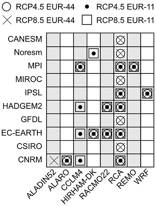
Figure 1. GCM/RCM matrix for the EURO-CORDEX experiments used in this paper.

Figure 2 shows the EURO-CORDEX domain and the sub-domains used in this study, with subdomain 6 slightly modified compared to Christensen and Christensen (2007). The analysis on sub-domains is performed to enhance the understanding of regional-to-local signals. Only aggregated results combining RCP4.5 and RCP8.5 are shown; however, analyses suggest (not shown) that no significant differences exist between RCP4.5 and RCP8.5 after scaling, as also shown globally by Tebaldi and Arblaster (2014) and regionally for Europe, as in the present study, in Christensen et al. (2019).

FIGURE 2

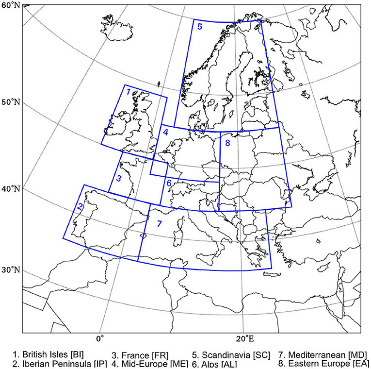
Figure 2. Cordex domain for Δx= 0.44° and Δx= 0.11° and the associated sub-domains.

2.2. Methods

2.2.1. The Pattern Scaling Approach

The pattern scaling is defined as the climate change of a 20-year mean (relative to 1985–2004) of the temperature and precipitation fields scaled by the global mean temperature change of the relevant GCM. In this study, the end-century scaled pattern is defined as the one calculated from 2080 to 2099, the latest period available for all models, divided by the time averaged global mean temperature change for the period.

2.2.2. The What-If Approach

The procedure used in the what-if approach is straightforward, as it extracts the year where the GCM in question, for all GCM-RCM combinations, crosses the selected climate change thresholds of 1, 2, and 3°C, respectively, at the first occurrence. We have not observed any multiple crossings, so this definition is unique here. Around the extracted years, a 20-year time average was then calculated from each model member combination followed by averaging all the members. Note that the scale of all patterns extracted by the what-if approach is adjusted to 1°C value (for example, the resulting 3°C pattern was divided by three).

2.2.3. Signal-To-Noise Ratio

As presented in Christensen et al. (2019), the S/N is produced for each scaled pattern output combination and on the results from the what-if approach. The S/N is defined as:

$\begin{array}{rc}S/N=\frac{<SP>}{{\sigma }_{SP}},& (1)\end{array}$

where <SP> is the scaled patterns average of all the members and σ_SP is the inter-member (32 members for EUR-11 and 35 members for EUR-44; see Figure 1) standard deviation of the scaled patterns from the net model results (i.e., there is no inter-annual variability component in this noise). The S/N is considered a good proxy of the robustness of the signal. When S/N > 1, the level of change is identified as significant change. It is worth noting that precipitation results are shown for relative changes (in %) unless stated otherwise.

3. Results

3.1. Scaled Pattern at the End of the Century

The end-of-century scaled patterns for temperature in DJF (first two rows of Figure 3) are showing strong warming in the north-east of the domain with a smaller value over the Atlantic Ocean as also observed by other studies (Christensen et al., 2015, 2019). However, although some larger differences can be observed in the S/N, the percentage of grid points where S/N < 1 (shown in the upper-left corner of each figure) is quite small if not zero. Only the area over the Atlantic Ocean is affected by S/N < 1 due to a moderate climate change signal. Note that EUR-44 is slightly warmer than the EUR-11. This is caused by the slightly different model ensembles available. Employing only models and hence identical model ensembles for the two resolutions, the scaled patterns between EUR-11 and EUR-44 do not show differences in temperature (not shown).

FIGURE 3

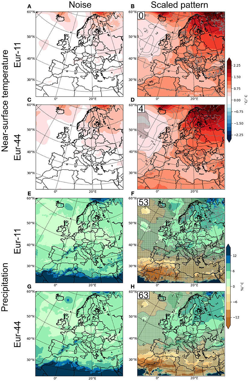
Figure 3. Scaled 2080–2099 DJF patterns for combinations of temperature (A–D)/precipitation (E–H) and EUR-11 (A,B,E,F)/EUR-44 (C,D,G,H). The left column shows the inter-member noise and the right column shows the 2080–2099 scaled patterns. The contour lines shown in the right column show the S/N ratio and the gray shading depicts areas of S/N < 1. The numbers in the upper left corner of the right column shows the percentage of grid points where S/N < 1. Note that both columns have the same unit.

The scaled patterns of the precipitation fields for DJF (last two rows of Figure 3) are showing, overall, a future with a wetter climate over northern Europe and drier conditions over the southern and north-western parts of the domain; the S/N ratio is quite similar. However, the percentage of grid points with S/N < 1 is considerably higher for precipitation (53, 63% for EUR-11 and EUR-44, respectively) indicating a higher disparity between ensemble members. In general, Northern European land areas have S/N larger than one. This is consistent with the global tendency of increased intensity of the hydrological cycle with global warming. The results show relatively low-level noise over the European region and a larger signal over the Scandinavian and Russian area. The low-level noise over the European continent is likely due to the large-scale circulation constraint dominating this mid-latitude region in this season (stratiform precipitation from large low-pressure systems) (Sørland et al., 2018).

The scaled patterns of JJA temperature (Figure 4) is showing a more homogeneous warming over the domain than DJF with the highest warming rates in the southern and northeastern parts of the domain as also observed in Christensen et al. (2019). In general, the JJA scaled precipitation patterns have a smaller S/N than those for DJF. Due to large inter-member disparities as seen here for JJA, as likely affected by the reproduction of convective precipitation, the percentage of grid points with S/N < 1 is higher (78, 83% for EUR-11 and EUR-44, respectively) than for DJF. The area where S/N > 1 over the Iberian Peninsula it is due to a stronger signal. It is expected that noise levels are higher in summer than in winter, as weather is more locally generated, which also means that the role of the regional model for noise is higher than in winter; this was originally described by Déqué et al. (2007). Further discussions on the robustness in relation to S/N is seen in section 3.4. The large levels of noise for JJA and DJF in the southern parts of the domain are related to the use of relative rather than absolute changes. This is supported by both a small absolute signal and a small absolute noise for this region (see Figure 12).

FIGURE 4

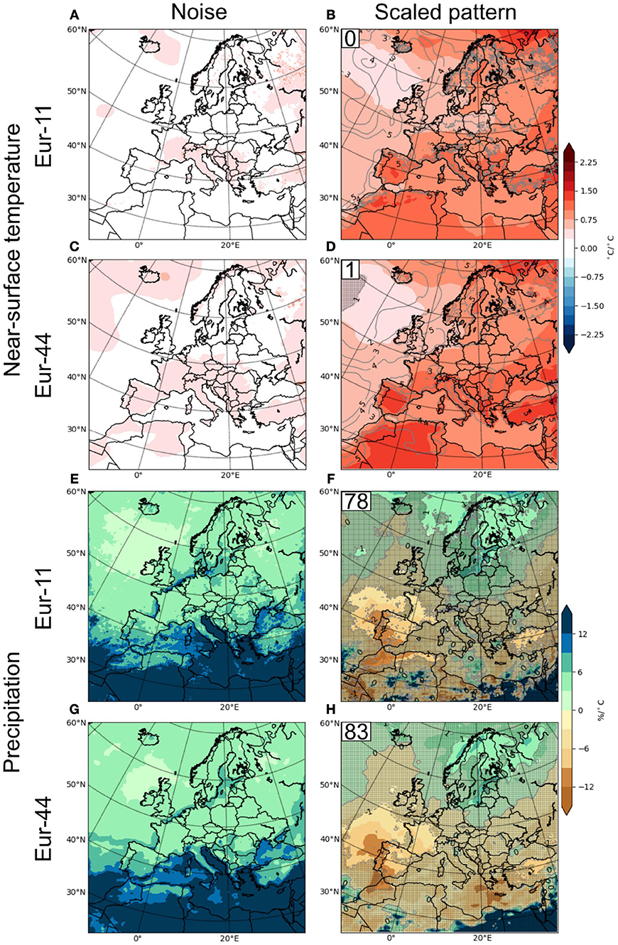
Figure 4. As for Figure 3 but for JJA.

The results presented in this section are similar to those presented in previous studies (Tebaldi and Arblaster, 2014; Christensen et al., 2015, 2019). In order to study the what-if approach, a deeper investigation of the evolution of the emerging scaled patterns is needed.

3.2. Emergence of the End-Of-Century Scaled Pattern

This section is focusing on the emergence of the scaled patterns. To depict the emergence of the scaled patterns, movies are available in the Supplementary Material showing the temporal evolution of the temperature and the scaled precipitation patterns for JJA and DJF (see Supplementary Videos S1, S2, respectively). Figure 5 shows the main statistics of the annual evolution of the scaled patterns from 2005 to 2090 (i.e., the 2005 level is calculated from the 1995–2014 period and so forth). The main purpose is to show at which time the scaled patterns shown in section 3.1 emerge at various geographical locations and scales.

FIGURE 5

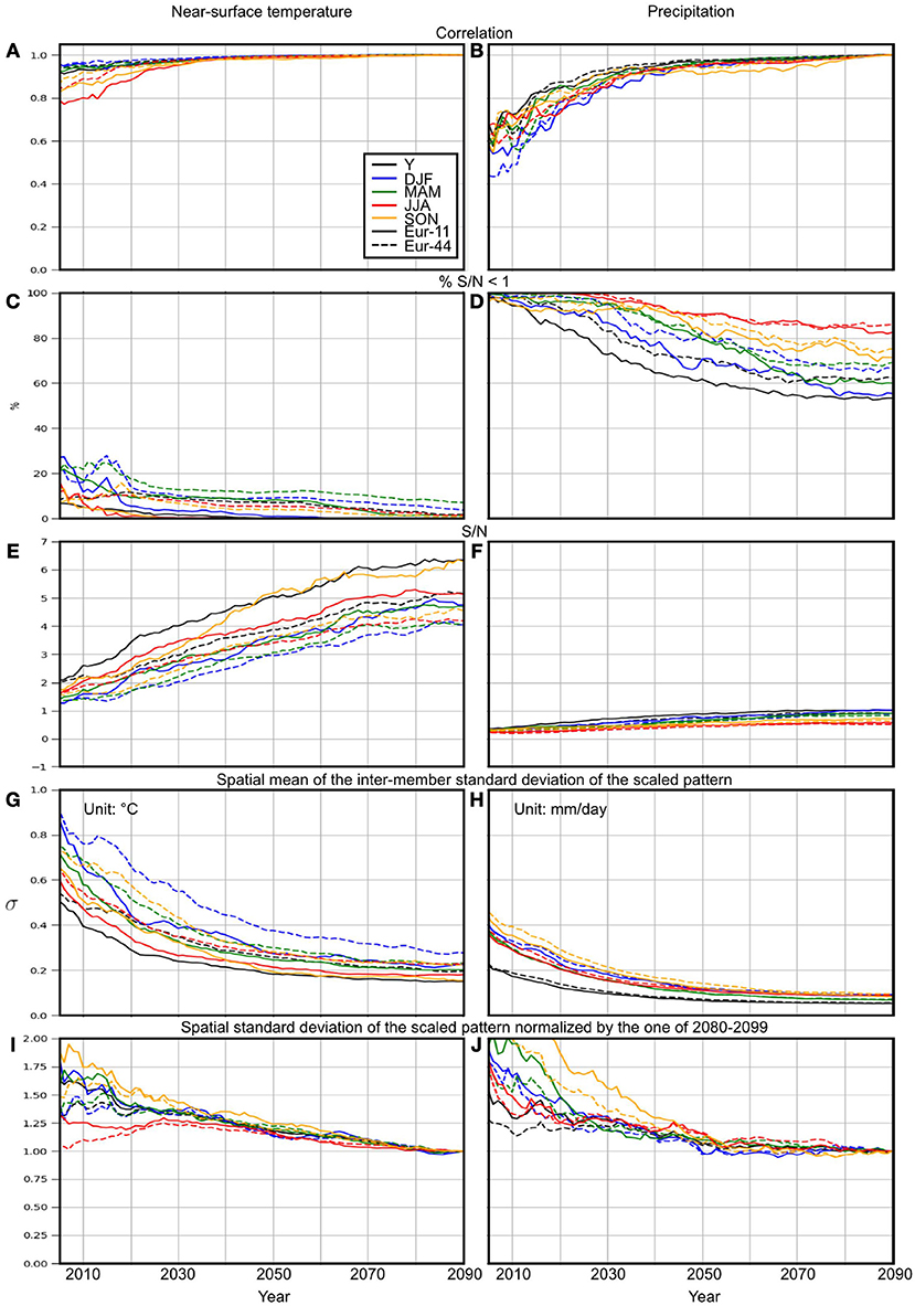
Figure 5. Correlation between a running mean of 20-years scaled patterns from 2005 to 2090 (central year shown) against corresponding end-period levels (2080–2099) (A,B). Percentage of grid points where S/N < 1 (C,D). Spatial average of the S/N levels (using the absolute signal) of the scaled patterns (E,F). Spatial average of inter-member standard deviation of the scaled patterns (G,H). Spatial standard deviation of scaled patterns normalized by that of 2080–2099 (I,J). The results are shown for both variables (temperature and absolute precipitation, left and right respectively), and across resolutions and seasons as well as annually.

The first row of Figure 5 shows the spatial correlation between the scaled patterns calculated each year against the 2080–2099 scaled patterns (as shown in Figures 3, 4). The spatial correlation for temperature (Figure 5A) reaches the asymptotic unit value for all seasons and for both resolutions early in the century (around 2035). The latest alignment to the asymptotic value is seen for the JJA season, which again is likely due to smaller-scale convective weather systems. For absolute precipitation change, the evolution of correlations (Figure 5B) is more divergent than for temperature, reaching unity at a later stage (around 2080). However, the correlation levels seem to stabilize around 2050. For precipitation, DJF is the last season to reach its asymptotic value.

The second and the third rows of Figure 5 show the percentage of grid points where S/N < 1 and the value of the spatial average of S/N, respectively. For temperature (Figure 5C), the percentage of grid points where S/N < 1 is relatively low early in the period. For EUR-11, a level of 0% is reached around 2040 whereas EUR-44 decreases to around 2% at the end of the century. The scaled precipitation patterns differ substantially from those of temperature (Figure 5D), starting at approximately 100% for all seasons and resolutions, decreasing steadily to levels between 50 and 85% at the end of the century. Accordingly, the spatial average of S/N is increasing for both variables (Figures 5E,F). At the start of the period, spatially averaged temperature S/N levels are already >1 reaching values between 4 and 6.4 at the end of the century (across seasons and resolutions) for temperature. However, although S/N levels also increase in precipitation, the spatial average is comparatively lower and shows a slower increase toward the end of the century, suggesting a much noisier field for precipitation. Note that the absolute signal has been used in order to avoid too large disparities due to use of relative value. The fourth row of Figure 5 depicts the spatial mean of the inter-member standard deviation of the scaled patterns. It is seen that regardless of variable, season and resolution, the inter-member disparity of the scaled patterns is larger in the beginning of the period and converges at the end of the century, which is in agreement with the results of the first rows of Figure 5. The last row of Figure 5 shows the spatial standard deviation of the ensemble mean scaled patterns normalized by the level at the end of the century. The results suggest that the spread between variables, seasons, and resolutions is higher early in the period, due to the large noise here, becoming increasingly similar toward the end of the century. The scaled precipitation patterns seem to converge to unity more rapidly than the temperature. This may be explained by the fact that warming over land is generally faster than the global average; therefore the mid-century is scaled by a smaller warming amplitude than the probably more relevant regional warming. As the sea catches up with the land during the century, this effect is diminished. Furthermore, the curves group together more rapidly than in the case of precipitation. In general, EUR-44 seems to differ somewhat from EUR-11 which is likely due to the slightly different sets of members between the EUR-11/EUR-44 model groups (not shown).

Although Figure 5 gives a general idea of the robustness of the signal in scaled patterns, Figure 6 shows that there are important local differences between the subregions. Figures 6A–H is showing the same as Figure 5D, but for land grid points of individual subregions (as shown in Figure 2), for all inland grid points (Figure 6I) and all water grid points (Figure 6J). Overall, all subdomains have more or less the same behavior; (1) levels of 100% is generally seen at the beginning decreasing toward the end of the century; (2) some large differences in seasons are seen with JJA showing the slowest decline; (3) DJF reaches the lowest levels (except for the Iberian Peninsula; Figure 6C).

FIGURE 6

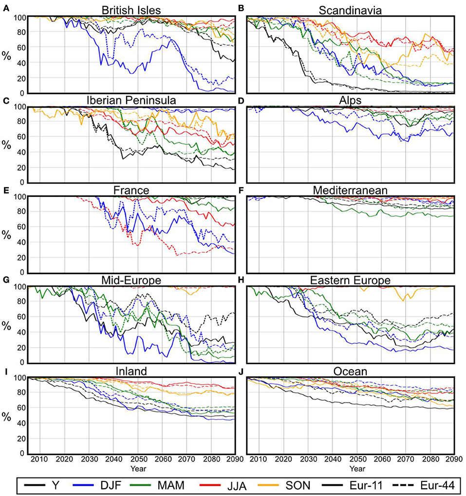
Figure 6. Percentage of inland grid points where S/N < 1 for absolute precipitation for each subdomain (A–H) and for land (I) and ocean (J) grid points in the full domain.

The high value shown for the Alps (Figure 6D) and the Mediterranean (Figure 6F) area is due to a persistently stronger noise (not shown) likely to be produced by the complex topography of the Alps and land/sea effects from the vast coastlines of the Mediterranean. Despite some variations in the evolution of the statistics and relatively low S/N, the movies (Supplementary Video S1) suggest that the underlying emerging patterns are already recognizable from around 2020.

3.3. Comparison Between the Pattern Scaling and the What-If Worlds

The main purpose of this section is to analyze the robustness and persistence of the scaled patterns by comparison to the patterns resulting from the what-if approach.

Figure 7 shows the global average of the ensemble mean of the 2 m temperature from the CMIP5 datasets used to drive the RCMs of this study. The years shown in the legend represent the year where the selected threshold is crossed by the global average of the ensemble mean. The 1°C threshold is crossed in 2031 and 2026, the 2°C is crossed in 2070 and 2050 for RCP4.5 and RCP8.5, respectively, and the 3°C is crossed in 2068 (RCP8.5 only). Overall, we have shown in section 3.2 that the signal increasingly emerges from the noise as we go through the century, which should be considered when comparing the scaled patterns from the patterns resulting from the what-if approach.

FIGURE 7

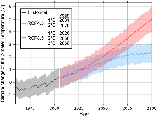
Figure 7. Global average of the ensemble mean of the 2-m temperature from the CMIP5 model used as driving data for this study. The black, blue, and red lines are the historical, RCP4.5 and RCP8.5, respectively. The shadow represents the standard deviation of the model ensemble. The years in the legend represent the year where the i°C was crossed by the global ensemble mean.

The mean what-if result at 1°C warming for JJA temperature (second column of Figure 8) shows a good correspondence (correlation of 0.93 and 0.97) with the scaled patterns for both resolutions (for Figures 8B,F, respectively), which was expected since the scaled temperature patterns converge rapidly (see Figure 5A). The results from the other two thresholds are also similar (showing pattern correlations of 0.98 [0.99] and 0.99 [0.99], respectively, for the 2 and 3°C thresholds for EUR-11 [EUR-44]; Figures 8C,D [Figures 8G,H], respectively). The main difference is seen in the percentage of grid points where S/N < 1 since EUR-11 (Figures 8A–D) shows levels of 0–1% for all temperature thresholds whereas EUR-44 (Figures 8E–H) shows a decrease from 7 to 0% with the increasing threshold from 1 to 3°C as also expected from Figure 5C. This is mostly due to a combination of low change signal and a large noise (Figures 4C,D). However, it is worth noting that the number of available members (lower-left corner) decreases as the threshold increases, since some simulations never reach the higher thresholds.

FIGURE 8

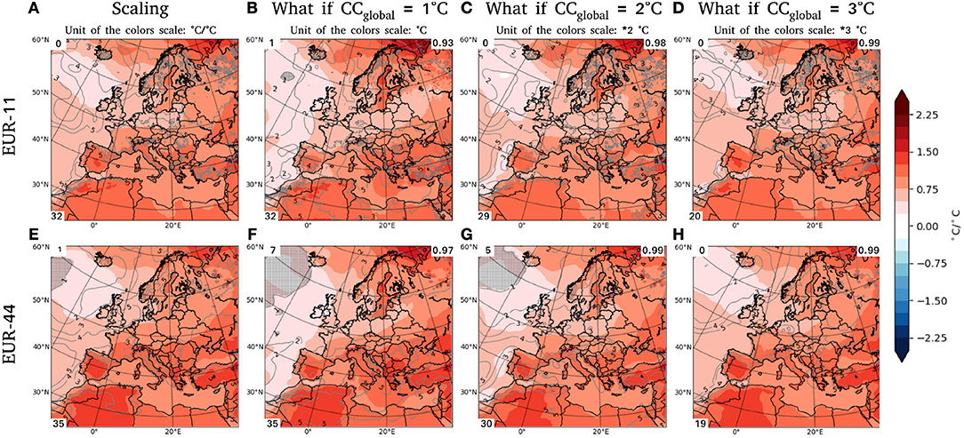
Figure 8. JJA temperature. 2080–2099 scaled fields (A,E), fields from the what-if approach for the 1°C (B,F), 2°C (C,G), and 3°C (D,H) for the EUR-11 domain and EUR-44 domain (A–D and E–H, respectively). The metrics shown in the corners of the figures include the percentage of grid points where S/N < 1 (upper left), the number of model members (lower left) and the correlation between the scaled pattern and the what-if approach (upper right for the what-if subplots). It is worth noting that the scale of the what-if patterns have to be multiplied by their threshold values to obtain actual warming.

For JJA precipitation (Figure 9), S/N is below 1 in 99% of the domain for the 1°C patterns making this scenario unusable (Figures 9B–F) for both resolutions. Also, the overall signal of the 1°C patterns differ from the scaled patterns [with correlations of 0.63 and 0.69 for EUR-11 and EUR-44, respectively (Figures 9B–F)] with the most notable differences south of the Baltic Sea, in the Mediterranean and in the southern parts of the domain. In contrast, the 2 and the 3°C patterns (third and fourth column of Figure 9) are showing a higher correlation than the 1°C pattern. However, in terms of correlation, little improvement is noted going from the 2°C to the 3°C level although some areas do improve such as the Baltic Sea and the Mediterranean area. The percentage of the S/N also decreases from 1, 2 to 3°C (99% [99%], 85% [86%], and 77% [76%], respectively for EUR-11 [EUR-44]) reflecting increasing confidence for a larger proportion of the domain. In summary, the 1°C patterns are likely unusable to reflect climate change patterns, leading to the conclusion that an analysis on 1°C should instead employ higher thresholds which are then subsequently adjusted to 1°C.

FIGURE 9

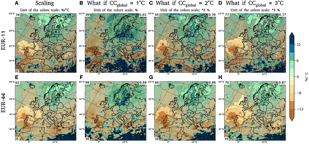
Figure 9. JJA precipitation. Specifications and conventions as in Figure 8.

For DJF temperature (Figure 10), as in JJA, the what-if pattern is similar to the scaled pattern (both resolutions) with a decrease in the percentage of grid points where S/N < 1 as the threshold increases. The S/N levels below 1 in the North Atlantic region is due to a small signal and a medium-to-large noise (not shown).

FIGURE 10

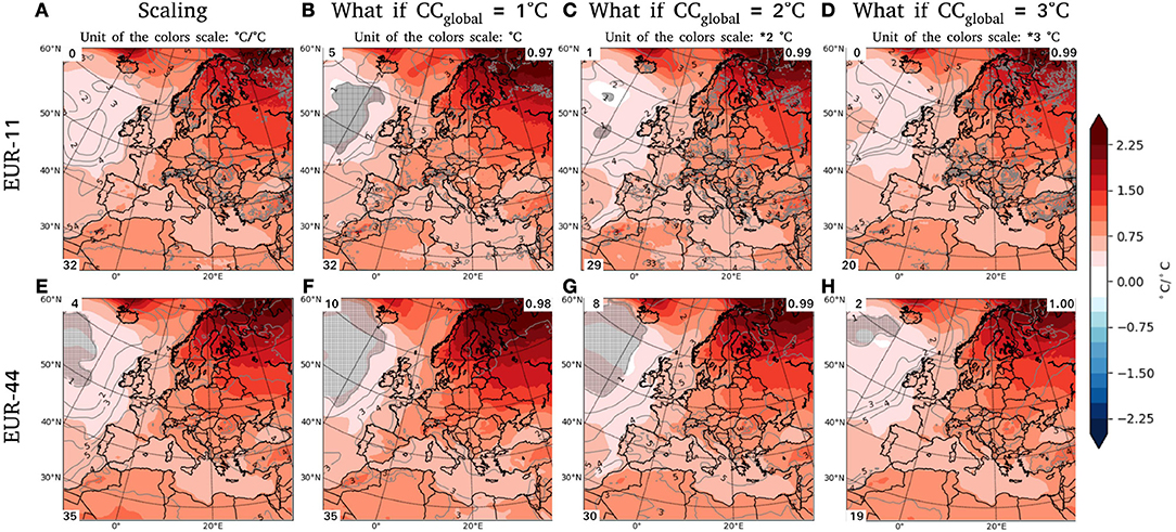
Figure 10. DJF temperature. Specifications and conventions as in Figure 8.

The 1°C patterns for DJF precipitation (second column of Figure 11) shows that the correlation is already high for 1°C and increases very little over the highest thresholds (both resolutions). Yet, the min/max values are distinct and become even more comparable when increasing the thresholds. Unlike the JJA 1°C precipitation pattern of EUR-11 (Figure 9B), DJF is showing a relatively large region where S/N > 1 over Germany, North Atlantic, the Norwegian Sea and North Algeria. The 2°C precipitation patterns have a relatively large area where S/N > 1 increasing to levels similar to the scaled patterns for the 3°C threshold for both resolutions.

FIGURE 11

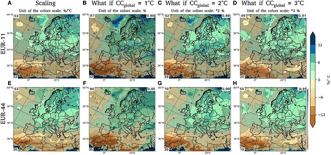
Figure 11. DJF precipitation. Specifications and conventions as in Figure 8.

In summary, the results suggest that patterns extracted from 1°C threshold should not be used whereas the scaled patterns shows a much more robust signal, which is similar to the 2 and 3°C patterns.

3.4. The Trustworthy Change Signal

In this study, we have defined the trustworthy information as the one where the main signal is detectable from the inter-model spread (S/N > 1). This is quite straightforward with temperature since S/N is almost always >1, except occasionally for the North Atlantic area. However, the quantity of information judged untrustworthy for the precipitation patterns is larger. The S/N metric might be misleading since negligible or small change signals are more likely to be judged as untrustworthy although usable information can in fact be extracted. McSweeney and Jones (2013) discuss this issue by using the interannual variability as noise and claim that a clear distinction should be made between “no signal” and a signal overwhelmed by noise. In this section, we wish to present some additional thoughts on this issue.

To deepen our understanding, several other metrics were selected and applied on the absolute field of precipitation. The first column of Figure 12 shows the inter-member noise of the scaled patterns. A bootstrap analysis with replacement using 1,000 samples was used to create 1,000 estimates of the noise. The resulting bootstrap average shows a similar, but weaker, pattern compared to those shown in Figures 3, 4. Furthermore, the 25th–75th range is quite narrow. The results together suggest that a few outlier members have a considerable impact on the noise, especially in the Alps and Mediterranean areas (confirmed by a qualitative visual evaluation).

FIGURE 12

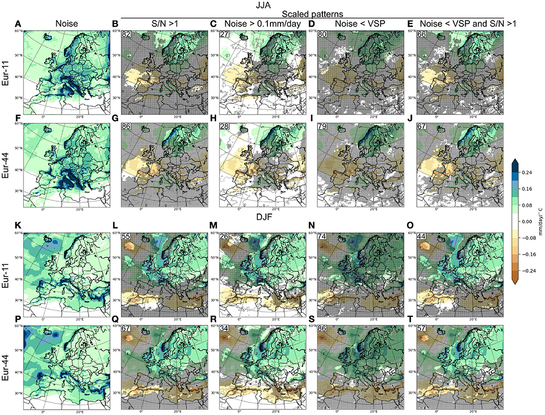
Figure 12. Inter-member noise (A,F,K,P) of the 2080–2099 scaled precipitation patterns where different thresholds have been used: (1) S/N > 1 (B,G,L,Q), (2) considering only grid points with Noise >0.1 mm/day (C,H,M,R), considering only grid points with Noise < VSP (D,I,N,S) and (4) considering only grid points with S/N > 1 together with Noise < VSP (E,J,O,T). The results are shown for JJA and DJF (A–J and K–T, respectively) and both resolutions for absolute precipitation. The contour lines show the S/N ratio and the gray shading depicts “low-trust” areas defined by the metric selected. In the upper left corner of each figure, the percentage of shaded grid points is shown.

As stated, it is expected that areas with high noise relative to the change signal should be judged untrustworthy; in that sense the S/N metric (second column of Figure 12—as also shown in Figures 9, 11) is suitable. But, using this metric, some regions are judged untrustworthy because of a combination of a weak signal and a weak noise (for example the Eastern part of the Mediterranean; subdomain 7 in Figure 2). Such weak noise should be considered when trying to extract a valuable signal. For the rest of the Mediterranean area the noise is large and the change signal weak, making it difficult to extract trustworthy information from this region.

The second metric used to judge the trustworthy information is to apply a quantitative threshold on the noise as shown here using 0.1 mm/day (third column of Figure 12), which in essence is a small change over a three month period (≈10 mm). By applying this threshold, numerous grid points become trustworthy in comparison with the conventional S/N approach (as shown by the decrease in the percentage of the untrustworthy grid points in the upper left of each figure) albeit still keeping all areas with high noise levels out of the trustworthy signal. The subjective selection of threshold level, however, might be disputable and it may also be region-specific.

The third metric is based on the Variability of the Scaled Patterns (VSP). The VSP is calculated by splitting the last 50 years of the scaled patterns evolution (from 2041 to 2090) into five decades (i.e., 2041–2050 and so forth). Using these five times slices an inter-decadal variability was calculated and then temporally averaged. The five decades are basically treated in the same way as would have been done with perturbed members for an internal variability study (see Lucas-Picher et al., 2008, for example). We interpret the VSP as the “natural” variability of the scaled patterns. So, all noise smaller than the VSP should not be considered. In Figure 12, the fourth column shows the available signal when not considering noise < VSP. This method has the advantage to produce trustworthy information using grid points with a low signal. Such an approach could be further complemented with the conventional S/N > 1 metric, which as shown in the fifth column of Figure 12. One can see that the resulting percentage of the available signal is higher than using the S/N metric, but less than using the 0.1 mm/day threshold. It is worth noting that a better description of VSP is needed to understand uncertainties related to scaled patterns.

4. Concluding Remarks

In this study, the robustness and scalability of regional climate projections over Europe have been studied using the EURO-CORDEX dataset. In the first section, the 2080–2099 scaled patterns of temperature and precipitation for DJF and JJA have been shown. In winter, the land is warmer than the ocean with a south-to-north warming gradient. During summer, the land is overall still warmer than the ocean and the warming is more homogeneous than in winter. The noise is smaller for temperature than precipitation for both seasons. In general, the noise is higher in the North Atlantic for all seasons in combination with a weak change signal resulting in areas where S/N < 1. The noise in precipitation is larger for the Alps and the Mediterranean, but weaker for the North Atlantic Ocean.

The second section analyzes the emergence of the scaled patterns, as also visualized in an animation (Supplementary Information). It has been shown that the scaled temperature patterns emerge faster than the corresponding patterns for precipitation. For temperature, the areas of trust (grid points where S/N > 1) increase to 100% toward the end of the century whereas a stabilization of 50–60% is seen for precipitation around 2050. The large noise throughout the century related to the scaled precipitation pattern suggests that the precipitation pattern is not as linear as is the case with temperature. However, although the signal drowns in the inter-member noise (the ratio of which decreases through the century), the consistency in the scaled precipitation patterns from 2020 suggests that the precipitation field is actually scalable at longer timescales.

The third section of the results shows a comparison between the scaled patterns and the pattern extracted from a what-if approach, where thresholds of 1, 2, and 3°C were employed. It has been shown that the patterns from the 2 and 3°C of the what-if approach results were highly similar to the end of century scaled patterns of temperature and also largely to the scaled precipitation pattern. The 1°C what-if patterns differed due to a lack of signal as elaborated below. It could also be seen (for both variables/seasons/resolutions) that the percentage of trustworthy grid points was increasing from the 1 to 2°C results and that no major differences were seen between 2 and 3°C and the scaled pattern. This latter result corresponds to the finding that patterns were stabilized around 2050. Nonetheless, patterns are already recognizable as early as 2020. The major difference was noted while comparing the 1°C precipitation patterns with the scaled ones. The percentage of trustworthy information is almost 0 for the 1°C results and the patterns were poorly represented. This suggests that patterns extracted from analyses with a 1°C threshold should not be used, whereas scaled patterns provide a more robust signal, as do 2 and 3°C patterns. It is worth noting that, although the pattern scaling approach provided important and robust information about the future climate change, this approach does not take into account any non-linear feedback from global warming. Those feedbacks might have a non-negligible impact on pattern scaling whereas processes with longer time scales (e.g., soil processes and permafrost in particular; Christensen 1999; Stendel and Christensen 2002) might be a reason for caution for longer projections and scales of the presented results. In Christensen et al. (2015), the scalability of regional climate signals with global temperature change was studied, and only extreme precipitation showed any strong deviation from linearity in this connection. In taking a pattern scaling approach, as many simulated climate change signals as possible are included, which is a direct way to improve the signal-to-noise ratio suppressing low-frequency variability.

Finally, the last results section is an attempt to raise the challenging issue of the “level of trust” in using a multi-model ensemble climate change signal. At first, the conventional metric S/N was used. It has, however, been suggested that this latter metric might misjudge information where a low-level change signal is located. Therefore, to deepen our understanding, an arbitrary threshold was applied to the noise resulting in increased levels, or areas, of trustworthy information. Only high noise regions, such as the Alps and the Mediterranean, remained below the trust level threshold. To overcome arbitrariness in the selection of this threshold, the variability of scaled patterns was calculated and used as a new threshold for the noise. It has been shown that when this threshold is combined with the conventional S/N, low-level signals, which were otherwise judged as unusable, become available as trustworthy change information. This study shows that pattern scaling can be used to analyze low- to high-level climate change signals with sufficient robustness for climate adaptation and mitigation for the likely climate evolution through the century.

Data Availability Statement

All data used in this study are available on the Earth System Grid Federation website (https://esg-dn1.nsc.liu.se/projects/esgf-liu/).

Author Contributions

JHC conceived the idea. DM led the study, processed the model data, performed the analysis, led the writing, and produced the figures. JHC, DM, MADL, and OBC analyzed the results, contributed to discussions, and the writing of the paper.

Funding

The research leading to these results has received funding from the European Research Council under the European Community's Seventh Framework Programme (FP7/2007-2013) ERC grant agreement 610055 as part of the ice2ice project. This work also received support by the European Union under the Horizon 2020 Grant Agreement 776613, the EUCP project.

Conflict of Interest Statement

The authors declare that the research was conducted in the absence of any commercial or financial relationships that could be construed as a potential conflict of interest.

Acknowledgments

We acknowledge the World Climate Research Programme's CORDEX project for its role in making available the WCRP CORDEX multi-model data set, and we thank the climate modeling groups for producing and making available their model outputs. The authors are grateful to the two reviewers that helped improve this manuscript.

Supplementary Material

The Supplementary Material for this article can be found online at: https://www.frontiersin.org/articles/10.3389/fenvs.2018.00163/full#supplementary-material

References

Christensen, J. H., Carter, T. R., and Giorgi, F. (2002). PRUDENCE employs new methods to assess European climate change. EOS Trans. Am. Geophys. Union 83:147. doi: 10.1029/2002EO000094

CrossRef Full Text | Google Scholar

Christensen, J. H., and Christensen, O. (2007). A summary of the PRUDENCE model projections of changes in European climate by the end of this century. Clim. Change 81, 7–30. doi: 10.1007/s10584-006-9210-7

CrossRef Full Text | Google Scholar

Christensen, J. H., Kjellström, E., Giorgi, F., Lenderink, G., and Rummukainen, M. (2010). Weight assignment in regional climate models. Clim. Res. 44, 179–194. doi: 10.3354/cr00916

CrossRef Full Text | Google Scholar

Christensen, J. H., Larsen, M. A. D., Christensen, O. B., Drews, M., and Stendel, M. (2019). Robustness of European climate projections from dynamical downscaling. Climate Dyn.

Google Scholar

Christensen, O. B. (1999). Relaxation of soil variables in a regional climate model. Tellus A 51, 674–685. doi: 10.3402/tellusa.v51i5.14486

CrossRef Full Text | Google Scholar

Christensen, O. B., Yang, S., Boberg, F., Maule, C. F., Thejll, P., Olesen, M., et al. (2015). Scalability of regional climate change in europe for high-end scenarios. Clim. Res. 64, 25–38. doi: 10.3354/cr01286

CrossRef Full Text | Google Scholar

Déqué, M., Rowell, D. P., Lüthi, D., Giorgi, F., Christensen, J. H., Rockel, B., et al. (2007). An intercomparison of regional climate simulations for Europe: assessing uncertainties in model projections. Clim. Change 81(Suppl. 1), 53–70. doi: 10.1007/s10584-006-9228-x

CrossRef Full Text | Google Scholar

Evans, J. P., and McCabe, M. F. (2013). Effect of model resolution on a regional climate model simulation over southeast Australia. Clim. Res. 56, 131–145. doi: 10.3354/cr01151

CrossRef Full Text | Google Scholar

Giorgi, F., and Gutowski, W. J. (2015). Regional dynamical downscaling and the CORDEX initiative. Annu. Rev. Environ. Resour. 40, 467–490. doi: 10.1146/annurev-environ-102014-021217

CrossRef Full Text | Google Scholar

Gutowski, J. W. J., Giorgi, F., Timbal, B., Frigon, A., Jacob, D., Kang, H., Raghavan, K., et al. (2016). WCRP COordinated Regional Downscaling EXperiment (CORDEX): a diagnostic MIP for CMIP6. Geosci. Model Dev. 9, 4087–4095. doi: 10.5194/gmd-9-4087-2016

CrossRef Full Text | Google Scholar

Harris, I., Jones, P. D., Osborn, T. J., and Lister, D. H. (2014). Updated high-resolution grids of monthly climatic observations-the CRU TS3. 10 Dataset. Int. J. Climatol. 34, 623–642. doi: 10.1002/joc.3711

CrossRef Full Text | Google Scholar

Huntingford, C., and Cox, P. M. (2000). An analogue model to derive additional climate change scenarios from existing GCM simulations. Clim. Dyn. 16, 575–586. doi: 10.1007/s003820000067

CrossRef Full Text | Google Scholar

IPCC (2007). Climate Change 2007: Contribution of Working Group 1 to the Fourth Assessment Report of the Intergovernmental Panel on Climate Change. eds S. Solomon, D. Qin, M. Manning, Z. Chen, M. Marquis, K. B. Averyt, M. Tignor, and H. L. Miller, Cambridge University Press.

IPCC (2018). Special Report on the Impacts of Global Warming of 1.5 °C.

Jacob, D., Petersen, J., Eggert, B., Alias, A., Christensen, O. B., Bouwer, L. M., et al. (2014). EURO-CORDEX: new high-resolution climate change projections for European impact research. Reg. Environ. Change 14, 563–578. doi: 10.1007/s10113-013-0499-2

CrossRef Full Text | Google Scholar

Knutti, R., Rogelj, J., Sedláček, J., and Fischer, E. M. (2016). A scientific critique of the two-degree climate change target. Nat. Geosci. 9:13. doi: 10.1038/ngeo2595

CrossRef Full Text | Google Scholar

Larsen, M. A., Christensen, J. H., Drews, M., Butts, M. B., and Refsgaard, J. C. (2016). Local control on precipitation in a fully coupled climate-hydrology model. Sci. Rep. 6:22927. doi: 10.1038/srep22927

PubMed Abstract | CrossRef Full Text | Google Scholar

Lucas-Picher, P., Caya, D., de Elía, R., and Laprise, R. (2008). Investigation of regional climate models internal variability with a ten-member ensemble of 10-year simulations over a large domain. Clim. Dyn. 31, 927–940. doi: 10.1007/s00382-008-0384-8

CrossRef Full Text | Google Scholar

Lustenberger, A., Knutti, R., and Fischer, E. M. (2014). The potential of pattern scaling for projecting temperature-related extreme indices. Int. J. Climatol. 34, 18–26. doi: 10.1002/joc.3659

CrossRef Full Text | Google Scholar

McSweeney, C. F., and Jones, R. G. (2013). No consensus on consensus: the challenge of finding a universal approach to measuring and mapping ensemble consistency in GCM projections. Clim. Change 119, 617–629. doi: 10.1007/s10584-013-0781-9

CrossRef Full Text | Google Scholar

Meehl, G. A., Covey, C., Delworth, T., Latif, M., McAvaney, B., Mitchell, J. F. B., et al. (2007). The WCRP CMIP3 multimodel dataset: a new era in climate change research. Bull. Am. Meteorol. Soc. 88, 1383–1394. doi: 10.1175/BAMS-88-9-1383

CrossRef Full Text | Google Scholar

Mitchell, T. D. (2003). Pattern scaling: an examination of the accuracy of the technique for describing future climates. Clim. Change 60, 217–242. doi: 10.1023/A:1026035305597

CrossRef Full Text | Google Scholar

New, M., Liverman, D., Schroder, H., and Anderson, K. (2011). Four degrees and beyond: the potential for a global temperature increase of four degrees and its implications. Philos. Trans. R. Soc. Lond. A Math. Phys. Eng. Sci. 369, 4–5. doi: 10.1098/rsta.2010.0304

CrossRef Full Text | Google Scholar

Peters, G. P., Andrew, R. M., Boden, T., Canadell, J. G., Ciais, P., Le Quéré, C., et al. (2012). The challenge to keep global warming below 2°c. Nat. Clim. Change 3:4. doi: 10.1038/nclimate1783

CrossRef Full Text | Google Scholar

Rae, J., Adalgeirsdóttir, G., Edwards, T., Fettweis, X., Gregory, G., Hewitt, H., et al. (2012). Greenland ice sheet surface mass balance: evaluating simulations and making projections with regional climate models. Cryosphere 6, 1275–1294. doi: 10.5194/tc-6-1275-2012

CrossRef Full Text | Google Scholar

Sanderson, M. G., Hemming, D. L., and Betts, R. A. (2011). Regional temperature and precipitation changes under high-end (≥4 c) global warming. Philos. Trans. R. Soc. Lond. A Math. Phys. Eng. Sci. 369, 85–98. doi: 10.1098/rsta.2010.0283

PubMed Abstract | CrossRef Full Text | Google Scholar

Santer, B. D., Wigley, T. M. L., Schlesinger, M. E., and Mitchell, J. F. B. (1990). Developing Climate Scenarios From Equilibrium GCM Results. Report Max Planck Institut für Meteorologie, Max-Planck-Institut fr Meteorologie.

Schwartz, C. S., Kain, J. S., Weiss, S. J., Xue, M., Bright, D. R., Kong, F., et al. (2010). Toward improved convection-allowing ensembles: model physics sensitivities and optimizing probabilistic guidance with small ensemble membership. Weather Forecast 25, 263–280. doi: 10.1175/2009WAF2222267.1

CrossRef Full Text | Google Scholar

Sørland, S. L., Schär, C., Lüthi, D., and Kjellström, E. (2018). Bias patterns and climate change signals in gcm-rcm model chains. Environ. Res. Lett. 13:074017. doi: 10.1088/1748-9326/aacc77

CrossRef Full Text | Google Scholar

Stendel, M., and Christensen, J. (2002). Impact of global warming on permafrost conditions in a coupled gcm. Geophys. Res. Lett. 29, 10–11. doi: 10.1029/2001GL014345

CrossRef Full Text | Google Scholar

Stocker, T. F. (2013). The closing door of climate targets. Science 339, 280–282. doi: 10.1126/science.1232468

PubMed Abstract | CrossRef Full Text | Google Scholar

Taylor, K. E., Stouffer, R. J., and Meehl, G. A. (2012). An overview of CMIP5 and the experiment design. Bull. Am. Meteorol. Soc. 93, 485–498. doi: 10.1175/BAMS-D-11-00094.1

CrossRef Full Text | Google Scholar

Tebaldi, C., and Arblaster, J. M. (2014). Pattern scaling: its strengths and limitations, and an update on the latest model simulations. Clim. Change 122, 459–471. doi: 10.1007/s10584-013-1032-9

CrossRef Full Text | Google Scholar

UNFCCC (2009). Decision 2/cp.15 Copenhagen Accord.

Van der Linden, P., and Mitchell, J. e. (2009). ENSEMBLES: Climate Change and Its Impacts-Summary of Research and Results from the ENSEMBLES Project. Exeter: Met Office Hadley Centre.

Google Scholar

Van Weverberg, K., Vogelmann, A. M., Lin, W., Luke, E. P., Cialella, A., Minnis, P., et al. (2013). The role of cloud microphysics parameterization in the simulation of mesoscale convective system clouds and precipitation in the tropical western Pacific. J. Atmos. Sci. 70, 1104–1128. doi: 10.1175/JAS-D-12-0104.1

CrossRef Full Text | Google Scholar

Vautard, R., Gobiet, A., Sobolowski, S., Kjellström, E., Stegehuis, A., Watkiss, P., et al. (2014). The European climate under a 2°C global warming. Environ. Res. Lett. 9:034006. doi: 10.1088/1748-9326/9/3/034006

CrossRef Full Text | Google Scholar