Abstract
Recent decades have been characterized by a rapid and steady urbanization of the global population. This trend is projected to remain stable in the future and to affect land use patterns in multiple ways. Monitoring and measurement concepts for urbanization processes have presented difficulties with the multitude of driving forces and variations in urban form as well as the assessment of outcomes of sometimes contradictory objectives for economic, social, and environmental policies. The monitoring frameworks that are employed with the aim of assessing the land use changes related to urbanization break down this complexity into singular dimensions that can be measured with individual indicators. Such monitoring allows planners and policy analysts to assess new urban growth against sustainable development criteria. Examples include compact city policies that allow urbanization to happen in suitable locations rather than laisser-faire urbanization that can happen regardless of environmental impacts and resource efficiency. In this context, we note that monitoring methods are most often designed for case studies in Europe or North America where urban structures are rather mature and consolidated. However, such monitoring can provide crucial information on urban development at a phase at which structures are currently evolving and can potentially still be modified. This is frequently the case in developing countries. Given this background, this paper presents an approach to simplifying the measurement of the land use changes related to urbanization with a new methodology. This paper condenses the needed measurement components into two dimensions: land use inefficiency and dispersion. The method can be used globally based on the newly available Global Human Settlement (GHS) layer that is available from the European Commission at no cost. In an initial application of the method to over 600 cities worldwide, we show the land use trends related to urbanization by continent and city size. In summary, we observe a consolidation of urban centers worldwide and continued sprawl on the outskirts. In European cities, a consolidation phase of urban structures began earlier, and cities are more mature and develop less dynamically compared to those in other regions of the world. More in-depth analyses of case studies present results for Paris, France, and Chicago, United States. In the case of Paris, the method helps to illustrate the growth pressures that led to massive urban sprawl on the outskirts with a continued densification of the inner city. In the case of Chicago, we observe a type of urban sprawl that goes along with the waves of suburbanization with population loss in the inner city and continued urban sprawl on the outskirts that are consolidated over time.
Introduction
Urbanization has been a megatrend of global land use change that can be observed in all parts of the world. By 2050 close to 70% of the global population will live in cities (Eurostat, 2016). The reasons that explain why the global population is more attracted to city life than ever have been widely discussed in the literature (see for example Adli, 2017). Many lines of argumentation suggest the so-called “urban advantage” that drives urbanization: city life is associated with better prospects for prosperity and progress, access to services, education, and amenities, as well as a richer cultural life. However, from a sustainability point of view, this promise may only hold true for the most attractive inner city locations where the distances between destinations are walkable, public transportation is good, and there is a density of people and activities result in what is perceived as urbanity. As a matter of fact most urban growth happens in the surrounding areas: We are living on a “suburban planet” and are trying to “make the world urban from the outside in” (Keil, 2017). These processes are not uniform though, the dichotomy between spatial categories has increasingly been contested over the last years. Suburbanization can have functional subcenters of high urbanity, peri-urban areas can consolidate over time to dense urban fabric, rural areas have centers with urban cores, and a high level of centrality and service quality (Hugo, 2017). The continuum between urban and rural areas becomes even more blurry in polycentric regions, where networks of cities form large metropolitan areas that exhibit a diverse set of land uses and urban functions (Danielzyk et al., 2016). It is increasingly becoming difficult for applications in urban land use monitoring to delineate functional urban areas in order to report on land use policies and related objectives. One such objective is to combat excessive forms of urban land take. This can be frequently observed in suburban areas, where the influx of people and the building activities that are needed to accommodate increased residential, industrial, and business land uses give rise to what is often labeled urban sprawl. The term “urban sprawl” has not yet been clearly defined. The term basically describes a form of urban growth whereby residential areas and social classes are highly segregated and dispersed over space, distances to amenities and workplaces can be comparatively long, and architecture lacks diversity (Galster et al., 2001; Wolman et al., 2005; European Environment Agency, 2006; Soule, 2006; Couch et al., 2007; Frenkel and Ashkenazi, 2008; Wei and Ewing, 2018). Urban theory concerned with sustainable planning has identified this form of urban growth as problematic. Expansions of urban areas should not be subject only to demand factors such as the housing preferences of the urban population or land market conditions. Planning regimes must manage urbanization with more foresight before unsustainable and irreversible urban sprawl structures are established to prevent the impacts of inefficient and environmentally harmful urban land use (Soule, 2006). Examples of such planning include urban containment policies or regional planning approaches that work with spatial concepts to optimize land use change (i.e., transit-oriented development or nodal growth, see Calthorpe and Fulton, 2001). Evidence-based policy aims to increase urban densities along development axis and nodes of good public transport accessibility and high quality service provisions, strengthening the links between the urban core and subcenters in such concepts. Favoring urban development in such a way is complemented by development restrictions in the interspaces between development axes. The objective of spatial planning in this line of thinking is to minimize the environmental impact of land conversions to sealed surfaces and ensure good outcomes for resource efficiency, accessibility and mobility and at the same time to prevent social imbalances with mixed-use urban design and affordable housing areas. The monitoring of these processes, however, is complex, since it is almost impossible to assess the causalities of land use change between the effects of spatial planning policies and global trends. Another difficulty is that such functional relationships are difficult to assess when analyzing land use change. Dedicated indicators that measure different aspects of dispersion, density, concentration, and other features of urban land use structures are typically employed to overcome this problem (Tsai, 2005; Herzig et al., 2018).
Early attempts to conceptualize sustainable urban development have identified three main characteristics, which are referred to as the three D's of urban development (diversity, density, and design, Cervero and Kockelman, 1997). Other researchers have enhanced this view and presented measurement concepts for urban sprawl. The work of Siedentop and Fina (2010), for example, takes a similar approach and focuses on the state and trends of land use in terms of surface features (urban land use change), patterns (urban land use structure), and density (population or business density). To date, the implementation of such measurement concepts has mainly been conducted in study areas in the Global North, using advanced geodata structures and population registers to calculate indices. Most scholars agree that there cannot be one combined index to measure urban sprawl. One must approach the topic with multiple criteria and indicators that capture the complexity of the different aspects that drive the land use change related to urbanization (Frenkel and Ashkenazi, 2008; Fina, 2013).
Global measurement concepts for urbanization have been studied in a meta-analysis by Seto et al. (2011). The authors look at 326 studies and applied four indicators of land expansion and population growth. In the results they identify the countries with the highest urbanization rates and analyzed correlations with factors like GDP growth or locational aspects. Zhang and Seto (2011) present an innovative way to display urban expansion in their research by using multi-temporal nighttime light data. This method allows for the differentiation between stable and highly dynamic urban areas, potentially defining urban growth rates for different countries. A more recently published way to present global urban growth is the Atlas of Urban Expansion (2019). Scientists from the New York University, the Lincoln Institute of Land Policy and UN Habitat developed an online visualization of urban land use for 200 cities worldwide. The project website contains information and visualizations of indicators suitable to differentiate between different types of urban form based on extent, density, and the composition of newly developed area. In our study we would like to conceptually advance and test such measures of urban form with a simplified approach that can be applied for multi-temporal data worldwide. Our main interest is to contribute toward monitoring concepts that detect and evaluate trends in urban development for global and regional land use dynamics.
In this context, this paper aims to use the knowledge generated by urban sprawl researchers in selected study areas and extend it to a global dataset that has only recently become available for a time series from 1975 to 2015. We use the global human settlement layers (GHSL) provided by the European Space Agency to calculate representative indices to measure urban growth worldwide. Based on these data, we establish a large database for each country with more than 5 million inhabitants. We apply the processing procedures for indicator calculations to the catchments of the cities with the highest urban land expansion rates in the observation period. To determine a valid logic for comparative analysis, we structure our sample by the selection of the fastest growing city regions in the classes of large, medium, and small cities (in terms of population size). We can thus assess some of the worldwide trends of land use change related to urbanization for growing cities. City borders are modeled using network analysis, taking travel times of up to 1 h in 15 min intervals as threshold values. This approach allows us to model catchments without arbitrary delineations of urban areas based on administrative boundaries. Monitoring applications for the largest urban regions in Germany conducted by the authors have shown that such delineation would not be realistic given the increasingly diverse mobility patterns of commuters. This is particularly true for polycentric city regions where the diversity of urban functions is increasingly becoming detached from theoretical conceptualizations of an urban-rural dichotomy (Fina et al., 2019). This methodology enables us to analyze the resulting land use characteristics in a comparative way, although some data inconsistencies explain deviations from the general logic.
These data and indicators provide the possibility of comparing the indicator results for world regions, planning regimes, or any other grouping logic in which urban researchers might be interested. However, the wealth of information is difficult to communicate and present. This paper therefore suggests a simplification procedure for urban growth assessments that concentrates on the dynamics of two dimensions: land use inefficiency and urban dispersion. We explain how the logic of this method was inspired by the discussion of existing quantification methods for urban sprawl represented in the literature. Subsequently, we apply the methodology in global observation and in two sample implementation areas (Paris, France, and Chicago, United States), including descriptions of the city selection procedure and indicators used. For the first applications of our methodological approach, we focus on the growth of cities and portray how the urban land use change has progressed in growing cities. We discuss interpretation prospects, methodological potentials and limitations as well as concepts for further research. By doing so, we hope to initiate discussion on the value of such a monitoring approach. In addition, the suggested approach could be a contribution to the spatial monitoring. Our two dimensional approach simplifies the measurement of urban form and provides policy makers and planning practitioners new information about regional and urban development trends, especially in terms of sustainable city development (United Nations, 2018).
Background
The growth of urban land use is a worldwide trend that threatens a range of ecosystem functions through the loss of vegetation and biodiversity, habitat functions, agricultural resources, and soil (Hasse and Lathrop, 2003; Haase et al., 2018). Such growth conflicts with climate change mitigation strategies in coastal locations that are susceptible and vulnerable to the effects of sea level rise and the higher frequency of extreme events (McGranahan et al., 2007). The actual impact of these effects varies; geographic conditions and specific sets of drivers of urban growth on global, regional and local scales as well as regulatory planning each play a role. There is a large consensus in the research community that some cities are more successful in terms of urban growth management than other cities (Fregolent and Tonin, 2015). In this respect, Tosics et al. (2010) classified the regulatory regimes of Europe in terms of land use controls and related it to the topic of urban growth. The authors basically consider the governance system to be either fragmented or consolidated and the planning policy system to have either strong or weak control at the regional or national governance levels. The findings of that study are instructive in comparing current planning systems across Europe but do not relate the findings to actual assessments of land use change in terms of urban growth. The influence of planning thus remains unknown, with some authors arguing that it may not be sufficiently effective to remedy the power of other driving forces in the context of urban sprawl. In this context, Angel et al. (2011) found that despite all planning efforts to control urban sprawl, such as compact city policies and urban growth management initiatives, urban land use change will continue to increase worldwide. The main reason for this increase is a rise in living standards that goes along with more land consumption per person. It is very rare that citizens dispense with less space for living and activities over time, although quite a few initiatives promote this way of thinking where high inner city density is proclaimed to be a factor for quality of life (see for example the OECD compact city policies, Organization for Economic Cooperation and Development, 2013). Besides the problems of decreasing densities in growing cities, Wolff et al. (2018) detected this process also in shrinking urban areas. As the demand (e.g., for infrastructure) decreases, shrinking cities are more challenged with dedensification than their growing counterparts. These efforts, however, are outmatched by a strong global trend for more land consumption. The most recent population prospects published by the United Nations shows that the main driver for more urban land, population growth, is expected to bring the global population from 7.7 million people in 2019 to 9.7 million in 2050, a 26% increase. This growth is expected to occur with varying rates across world regions, ranging from 99% increase in Sub-Saharan Africa to only 2% in Europe and North America. As a matter of fact, more than half of the projected growth is expected in only nine countries: India, Nigeria, Pakistan, the Democratic Republic of the Congo, Ethiopia, the United Republic of Tanzania, Egypt, and the United States of America. In contrast, 27 countries or areas are already experiencing population decline today, including the most populous country, China. Fertility rates are decreasing worldwide, so that population growth can actually reverse over the generations. The increase of life expectancy compensates for some of this dynamic, and some countries will see a high increase in elderly people over the next decades (United Nations, 2019).
With regard to the consequences of population growth for urbanization, any regulatory approach must be based on robust information about the current state and development trends of urban land use change. Beginning in the 2000s, a line of research focused on this topic with studies that have given considerable research attention to land use dynamics. Cervero and Kockelman (1997) showed how to identify the influential factors of urban form with a view toward travel demand. The landmark study by these authors on the influence of the “density,” “diversity,” and “design” of urban neighborhoods (the so-called “three D's”) inspired subsequent studies to work with multiple indicators to quantify urban land use patterns. In this line of thinking, authors such as Galster et al. (2001), Wolman et al. (2005), and Ewing and Rong (2008), established theories and measurement frameworks for urban sprawl assessments in the United States. These studies consider the drivers of urban sprawl and acknowledge the fact that the assessment of urban areas is very complex in terms of urban land use change. For example, Galster et al. (2001) identify eight criteria (density, continuity, concentration, clustering, centrality, nuclearity, mixed uses, proximity) related to land use and its distribution over an urban area for urban sprawl assessment in the United States. The criteria can be measured individually and are used in that study as inputs for a factor analysis to apply a form of multicriteria assessment for the ranking of US cities. Such rankings are useful for comparative analysis of development paths between cities but provide no normative information on the success of planning interventions or the criticality of urban sprawl in terms of its impacts. For such purposes, time series in monitoring frameworks dedicated to the testing of policy interventions are needed. In this context, the European Environment Agency inspired further research with a technical report on urban sprawl in 2006 in which it identified the challenges of measuring urban sprawl with a matrix of drivers that are differentiated by topic (land, transport, governance, economy, society) and scale (global, regional, local) (European Environment Agency, 2006). Subsequent state-of-the-environment studies adopted these ideas by applying a so-called pressure-state-response model to the assessment of undesirable land use changes, resulting in rather alarming qualitative assessments of urban sprawl perspectives for the near (five-plus years) and more distant (20-plus years) future (European Environment Agency, 2011, 2015). The measurement approach considers the interrelationships among the current state of land use, the driving forces that exert pressure on the system (for example, population growth), the actual impacts on ecosystem functions (in a normative assessment), and the effects of policies. Other work that was later taken up by the European Union to report on landscape fragmentation with a view toward urban sprawl adopted measurement methods based on landscape metrics. The aim was to assess the configuration and patterns of urban land use using geographic information systems (Siedentop, 2005; Jaeger and Bertiller, 2006; Jaeger et al., 2009; Siedentop and Fina, 2010; European Environment Agency, 2011; Fina, 2013; Behnisch et al., 2018).
Our interpretation of the literature is that the US literature seems to focus more on economic urban functions and their resource efficiency within cities (e.g., Galster et al., 2001) whereas the European literature is more concerned with the environmental impacts of urban sprawl (e.g., European Environment Agency, 2006). However, there is no clear research agenda that explains this observation, and there are certainly many overlapping areas. A range of indicators are presented in the literature to measure the degree of urban sprawl that are applied to geographic datasets on different scales, from a binary view of urban vs. non-urban land, to the study of the building blocks of different land uses, to analysis at the level of street addresses and types of households and enterprises. There are too many indicators to discuss in this paper. However, the common denominator of most measurement concepts is the use of selected indicators that represent different dimensions of urban land use change. In this context, the study by Galster et al. (2001) mentioned above was able to operationalize eight dimensions based on census block data in the United States. Such data structures are not available for international comparative analyses on such a detailed level. Some authors have therefore employed simplified measurements, grouping the dimensions with the most essential indicators. A research group from Switzerland worked with only three indicators to determine the amount of urban structures in a study area (“degree of urban permeation”), their locational setup (“degree of urban dispersion”) and the intensity of use that might justify a higher urbanization level (“sprawl per capita”; Jaeger et al., 2010). These authors combined the indicator values for their study area to only one measure (“total sprawl”). Frenkel and Ashkenazi (2008) work with three dimensions of urban sprawl (“density,” “scatter,” “mixture of land uses”), to which they refer as configuration and composition parameters. The indicators to operationalize these dimensions are as follows: population density, irregularity of the shape of the central built-up area boundary, fragmentation, land-use segregation, and land-use composition. Both of these studies require datasets that are not available everywhere. Similarly, a study from an environmental government institution in the German state of Baden-Württemberg suggested a measurement based on three dimensions that can be translated as density, efficiency, and quality of urban land use. This concept places explicit emphasis on indicators that detect changes over time in addition to indicators that measure the state of urban land uses at the beginning of an observation period (Landesanstalt für Umwelt, 2007).
Another example is the theoretical framework by Siedentop and Fina (2010) (see Supplementary Figure 1). This framework differentiates three dimensions of urban sprawl as being subject to singular indicator assessments. These dimensions include (1) surface characteristics, such as the amount of urban land use and its increase over time, the sealing degree of different urban land uses or the amount of urban green spaces and mixed land use functions. The resulting land use pattern (2) is the second dimension and addresses the configuration and position of different land uses toward one another as being dispersed or compact, fragmenting open space or forming planned and optimized structures, such as transit-oriented development or nodal growth. Urban density (3) considers the number of users in a given residential population, for example, based on their reliance on certain urban land uses, such as public transportation. In that case, more users would create a higher demand for such services, which would improve cost-efficiency.
The framework attributes certain impacts of urbanization to the sphere of influence of these dimensions (e.g., the loss/degradation of farmland, urban heat islands). Subsequent attempts to operationalize this concept have resulted in a challenging demand on data availability and time series consistency. The indicators that were implemented as representative are urban density; change in urban density; greenfield development rate (dimension: density); effective share of open space; patch density; mean shape index; openness index (dimension: pattern); and share of urbanized land and new consumption (dimension: surface). A full description would exceed the scope of this paper; however, references can be found in Siedentop and Fina (2010). Nevertheless, it is important to note that the pattern indicators are especially complex study objects in themselves. For example, the effective share of open space as a measure of landscape fragmentation is employed to reflect the value of habitat size for the health of flora and fauna. The resulting value is higher for large habitats and smaller for small habitats based on complex procedures to geographically extract habitat sizes among urban areas for a given study area and to assess the remaining connected size (Ackermann and Schweiger, 2008). The important aspect to note here is that many of the indicators presented in these studies can only be operationalized in administrations with advanced capacities to provide detailed geographic objects on urban land use and statistical data (e.g., on population development) on small-scale urban units. The results are convincing and promising; however, they cannot be extended to other regions with limited data availability. From this viewpoint, it is regrettable that monitoring methods are being designed in regions of the world with advanced data structures in rather mature and consolidated environments that cannot be easily applied where they are needed most, namely, in regions where urbanization is still very dynamic and information on the alarming trajectories of land use change could be used in crucial decision-making processes and adjustments to land use policies. In this context, Wei and Ewing (2018) recently published a call for new research efforts on the topic with a view toward capturing the variety of urban land use change worldwide. The following sections present a dataset that we tested in this context. These are worldwide data, and they provide a consistent time series from 1975 to 2015.
Materials and Methods
Land Use and Population Data
We use the GHSL as our main source for the analysis. This source, which is based on Landsat satellite and census data, is a dataset that is available worldwide. This dataset covers built land areas (built-up layer) and population data (population layer) for 1975, 1990, 2000, and 2015 (Pesaresi et al., 2013). The GHS built-up layer, with a high resolution of 38 m, provides the opportunity to monitor changes in urban land use and the resulting patterns using indicators that are applicable in a global context. In addition, we have information on population development from the GHS population layer on a 250 m cell size so that we can report on the demographic impact on urban growth. This data is available for 1975, 1990, 2000, and 2014 and stems from population estimation and disaggregation models (Freire et al., 2016). There are some caveats that come with the use of the dataset, although we generally assess it to be a unique source for the observation and analysis of global urban developments in the future. In their research, Pesaresi et al. (2016) described challenges and problems with the GHSL and its validation. A relevant issue for our study is that, due to a lack of available image data for 1975, there are problems in identifying built-up areas for this year. As the information of population is a result of the census data and the built-up layer, we also expect inaccuracies in the population dataset (see for the example of the German city of Pirmasens in Supplementary Table 25). We documented such inconsistencies found during data processing in the population (Supplementary Table 25) and in the remote sensing data (Supplementary Figure 2). This led to an exclusion of possible cities to analyse and to a drop in sample size (see Supplementary Table 3).
City Selection Procedure
To find a representative dataset of the most growing cities from different world regions, we defined a specific selection procedure. In a pre-analysis step, we used a 60 km buffer around every city centroid as a typical catchment for cities. The source is a point dataset provided by Esri and Garmin (Esri Word Populated Places), which contains a centroid for the administrative boundaries of every city with more than 50,000 inhabitants. This distance can generally be managed in 1 h travel time by car, which represents a maximum commuting time in Europe (Eurostat, 2019). We are aware that this not applicable for every country or city, but we need equal distances for our selection procedure. In comparison to the delimitation of functional urban areas of the urban audit, which includes employment and population data, we could identify similar catchment areas for the larger cities (Eurostat, 2013). As the research focus is set on cities with increasing urbanized areas, we concentrate on two kinds of city: those with most absolute growth and most relative growth in built-up land in city regions. The calculation of growth makes use of the GHS change layer of built-up areas and identifies the time period with the largest values from 1975 to 2015. Considering the fact that the most populated cities are often also the most growing cities, we decided to divide cities into three size classes: category A (over 500,000 inhabitants), category B (100,000–500,000 inhabitants) and category C (50,000–100,000 inhabitants). The information about the population classes is also part of the Esri world populated places with 2017 as reference year.
We also applied two filtering steps. The first approach eliminates the dataset entries for smaller countries, giving effect to the assumption that the growth of cities in small countries, such as Liechtenstein or Luxembourg, is highly influenced by neighboring metropolitan regions in other countries and does not provide the number of cities to present a solid selection base (e.g., small island country states, such as Samoa or Cape Verde). As a result, we excluded countries with fewer than 2 million inhabitants from this part of the research. To avoid agglomeration and overlap effects in polycentric urban regions—cities affecting the growth of catchments of neighboring cities—such as in the Ruhr area in Germany or the east coast of China, we implemented the second filtering rule: the cities of category A are not subject to any special restrictions. The cities of category B cannot be in a radius of 60 km from a city of category A. We dropped the cities of category C from the sample if they are in 60 km proximity to a larger city from categories A and B. Excluded cities remain part of the larger city region. Subsequently, the sample for a specific city category is filled with the next entry in the ordered list of growing cities in its category. For example, if a city of category B is part of the catchment of a city from category A, it will be part of the analysis for the larger city and will no longer be considered individually. Then, the city that is next in rank in category B is taken into consideration for spatial analysis. In its final state, the database contains a maximum of six cities per country, with the exception of smaller countries where many cities are geographically close to one another and affected by the application of filtering rules. As a result, some city categories are missing in such countries. For a total overview of all of the selected cities (see Supplementary Table 4).
Table 1 shows the resulting cities for the example of France. Of the largest cities, Paris had the highest absolute growth in hectares (4,614 km2 from 1975 to 2015), which is certainly due to its extraordinary size compared to the next-largest cities. However, in relative terms, Reims had a higher growth rate in percentage terms (150% from 1975 to 2015). For cities with 100,000–500,000 inhabitants, Lille had the highest absolute growth rate, Avignon had the highest relative growth rate. In category C (under 100,000 inhabitants) Saint Quentin had the highest absolute growth and Beziers the highest relative growth.
Table 1
| City/growth | Absolute | Relative |
|---|---|---|
| A (more than 500,000 population) | Paris (4,614 km2) | Reims (150%) |
| B (between 100,000 and 500,000 population) | Lille (3,554 km2) | Avignon (221%) |
| C (under 100,000 population) | Saint Quentin (1,208 km2) | Beziers (271%) |
Cities with the highest urban development dynamics in France, by population class (in brackets: absolute and relative change of urban land).
Processing and Analysis
Our logic for delineating catchments for cities uses travel time areas from the city centers as its core element. This approach reflects the functional relationships between the city center and its surroundings better than linear rings or squares. Processes of urbanization (e.g., sub- or re-urbanization) and related phenomena (i.e., commutersheds) rely on street networks. Indicators that measure such processes are therefore better calculated in alignment with network geographies. In particular, the analysis of urban growth will provide more realistic and comprehensible results in this context. Topographic features such as mountains, water surfaces, forests, or conservation areas are usually not accessible by road and were therefore intentionally excluded from the research area. If frozen boundaries were used, inaccessible or unconnected areas would also be part of the analysis. However, defining the catchment areas by travel time polygons also contains some deficiencies. Although indicators for cities can be compared, they are based on different geometry sizes in contrast to static squares or circles. We have to consider this in the interpretation of the results.
The resulting polygons represent so-called isochrones (polygons of equivalent travel time for the centroid) or spatial units such as those shown in Figure 1. The travel time polygon for the city of Innsbruck in Austria runs through the valley locations to the east, south, and west. Northern parts in the alpine valleys are more difficult to reach and thus take longer. Another example is shown on the right-hand side, which is located in the desert. The isochrones of Hafar al Batin in Saudi-Arabia span the first two rings, the outer rings are singular radial roads, which are officially labeled as highways, and other parts are not accessible by sealed roads (excluding dirt tracks). Unaffected by any topographic restrictions, the city of Dusseldorf in Germany approximates circular travel time rings, albeit with some deviations.
Figure 1
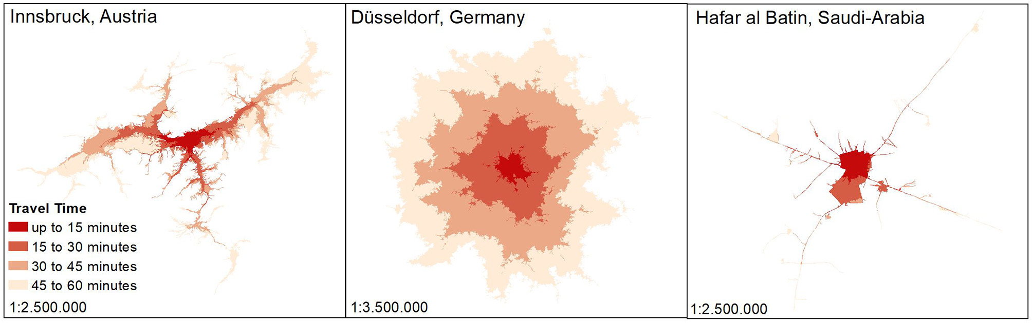
Examples of travel time polygons.
For our analysis of individual cities, we calculated isochrones for car travel times of 15, 30, 45, and 60 min to the city center. Data basis for the analysis is the ESRI ArcGIS Online network analysis services, which delivers “up-to-date” road data by HereMaps. With an almost worldwide available routing network, this source ensures our requirements for the analysis with a given reference year of 2018 (Esri, 2019). We use the resulting isochrones for all observation years to make the results comparable. For the application on the global level in section Global Observation, we simplify and aggregate the database by reducing the research area to a single catchment ring per city category. The travel time used to create the rings relies on city size. For the cities of category A (over 500,000 inhabitants), we assigned a travel time of 45 min; for the cities of category B (between 100,000 and 500,000 inhabitants), we assigned a travel time of 30 min; and for the cities of category C (<100,000 inhabitants), we assigned a travel time of 15 min. Restrictions such as toll roads or unpaved roads are ignored for this purpose because they prevent general accessibility and would have yielded unrealistic and complex isochrones, including islands, and possibly disconnected polygons. Such restrictions are therefore set to the minimum in the software we used, the ESRI ArcGIS Online network creation tool. Excluding toll roads or unpaved roads also leads to better results in the US and rural parts of Asia and Africa, where a large number of roads are actually unpaved. The only restriction we considered is the use of ferries to avoid areas that are inaccessible by car. Despite its good usability, there are some limitations in the use of Esri service areas. In general, there are problems in countries, such as North Korea, Afghanistan or Yemen, where the street network data do not seem to be very reliable and yielded inconclusive results (mainly visible in the form of the resulting polygons). In addition, there are potential problems when calculating drive time areas in smaller cities in Asia, Africa and South America, most likely also due to deficiencies in the available street network data. Countries and cities with inconclusive results had to be excluded from the city selection to avoid unrealistic indicator calculations. It is important to note that especially smaller cities in the named continents have outer rings with smaller areas. We suspect that the definition problems in street hierarchy and connectivity in rural areas are responsible for this issue. In the interpretation of the results, it is crucial to check the forms of the catchments to reflect the topographic conditions in the area. It is also important to note that the isochrones are valid for the recent past when the street network we used was in place. Therefore, for the previous years of our observation period, we may have potentially overestimated accessibility. From a methodological point of view, this is a necessary specification and provides a solid framework for the analysis of trends from the past. For future monitoring purposes, such fixed spatial units could impose restrictions when excessive growth renders these polygons outdated.
Indicators
As shown in the literature review the measurement and analysis of urban land use trends requires a multitude of indicators. According to the framework depicted in Supplementary Figure 1, multiple indicators are selected to represent the three dimension of growth (see Table 2): change of land surface characteristics (dimension 1), change of urban density (dimension 2), and change of land use patterns (dimension 3). The indicators we selected for our study can be implemented with the GHSL. With this background, we condensed the three dimensions of urban sprawl to only two dimensions: the dimensions of land use (in-) efficiency and dispersion.
Land use inefficiency: we borrowed this concept from a range of reporting tools on urban form but could not identify who published the idea first1; however, it is a simple comparison of population growth vs. urban area growth. If the population growth is higher, the urban footprint will become denser. If the population growth is much lower, the urban structure will become less dense, which is typical for urban sprawl. This dimension therefore measures the economic use of land resources over time in light of population development. This approach is sometimes labeled as land use efficiency, a term we adopt but invert the logic in terms of land use inefficiency to make our results more accessible in light of the indicator values. Land use efficiency is also an indicator in the United Nations Sustainable Development Goals and therefore highly relevant for policy formulation (Number 11, see United Nations, 2018; Florczyk et al., 2019). Put simply, land use inefficiency covers the dynamics of the surface and density dimensions.
Dispersion: we monitor and assess the pattern dimension with the changes observed for the so-called “dispersion index.” The methodology for this indicator was first presented by Taubenböck et al. (2018) with a very simple binary analysis of settlement and non-settlement areas. Dispersion index derives two spatial metrics from these land use classes, the largest patch, and the number of patches (McGarigal, 2015), and it positions these metrics in relation in one another. The share of the largest settlement patch in the entire area represents the dominance of one patch in a landscape. The number of patches equals the total number of all patches in the landscape. By normalizing the values of the number of patches and the largest patch, we obtain equal ranges from 0 to 100 (see Figure 2). Low values indicate a compact settlement structure, and high values indicate dispersion.
Table 2
| Indicator | Range | Calculation |
|---|---|---|
| Growth rate of built land per year (n) (BuiltGR) | (–∞) to (+∞) | |
| Growth rate of population per year (n) (PopGR) | (–∞) to (+∞) | |
| Land use inefficiency (LUI) | (–∞) to (+∞) | LUI = BuiltGR−PopGR |
| Dispersion index change (DIC) | −100 to + 100 | DIC = End DI−Start DI |
| Dispersion index (DI) | 0 to 100 | |
| Largest patch (normalized) (LPn) | 0 to 100 | |
| Largest patch (LP) | 0 to 100 | |
| Number of patches (normalized) (NPn) | 0 to 100 | |
| Number of patches (NP) | 0 to (+∞) | NP = NP (absolute) |
Overview of indicators and their calculation (gray = main indicators).
Figure 2

Example for urban land use patterns and the corresponding largest patch index (LPn), normalized number of patches (NPn), and dispersion index (DI) values (urbanized land in black, largest patch in red).
Based on these indicators, we can portray the development of a city in a two-dimensional matrix. On the y-axis, we translate the surface and density dimension of our measurement concept into a value for the land use inefficiency as a result of land consumption and population growth in a given time period. If the population and urban land use grow at similar rates, the land use inefficiency remains constant (see Figure 3). Urban land use change that exceeds population growth considerably is an indication of wasteful land use management and a decrease in urban density (“less dense” in Figure 3, upper two quadrants). If the population grows much more than the urban land use, we obtain densification and higher efficiency (“denser,” lower two quadrants).
Figure 3
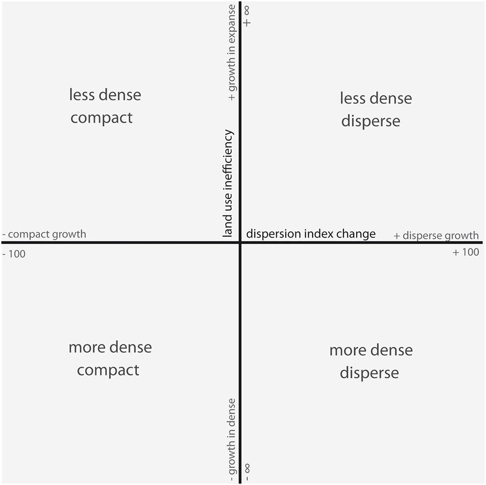
Trends of urbanization, divided into the four quadrants.
In other words, land use inefficiency measures the difference of built-up area growth in relation to population growth and indicates whether urban density is increasing or decreasing. The x-axis, in contrast, is defined by the development of the dispersion index over time. If urban areas grow from a very patchy (or “sprawling”) condition to more compact structures, the values will be negative (“more compact,” two quadrants toward the left). Accordingly, if new patches of urban land are built in isolation from existing urban areas, the dispersion (and urban sprawl) will increase (positive values), placing the value of the dispersion index change further to the right (two quadrants on the right-hand side).
Based on this idea, we can now depict the development of urban areas in terms of land use inefficiency and the change in the dispersion index in combination. A positive land use inefficiency value refers to less dense growth with a higher consumption of land; a negative land use inefficiency value refers to denser growth in the particular period. The objective of this approach is to portray the urban land use changes for the three time periods from 1975 to 1990, 1990 to 2000, and 2000 to 2015. To present the results on the full time series (1975 to 2015), we use the geometrical mean as the average of the growth rates between single time periods (e.g., 1975–1990, 1990–2000, 2000–2015). The complete mathematical definitions of the single indicators required to fill the land use inefficiency and dispersion index change matric is shown in Table 2.
Results
In the first step, we apply the introduced methodology on a global observation level. For this purpose, we work with only one catchment ring, simplifying outputs to one value for a city per year, categorized by city size classes.
Global Observation
The overview in Figure 4 shows the average values for urbanization trends by continent, taking the mean indicator values for each city type. The general development trajectories of urban land use change are comparable. Every continent exhibits a highly dynamic, less dense, and compact growth in the first period with some specific deviations. The growth development in Asia is more intense than, for example, in Europe, Australia and Africa. North and South American cities are characterized by a development compaction where the existing sprawling structures have been filled with new built-up areas over time; thus, urban footprints consolidate over the observation period and become denser. The time periods from 1990 to 2000 and 2000 to 2015 suggest that the growth dynamics on every continent have accelerated. Differences can be observed when examining the location of the darker red points in the quadrants of Figure 4. The growth dynamics in African cities do not lead to the same densification as on other continents, i.e., the land use inefficiency increases on the y-axis. At the same time, the growth curve in Asia moves across the quadrants to the 3rd quadrant, illustrating a compaction and densification of the urban footprint. In Australia, built areas change from being less dense and dispersed to denser and more compact. European urbanization since 1990 is characterized by a starting point that is already quite consolidated, i.e., closer to the zero points of the x- and y-axis in Figure 4.
Figure 4
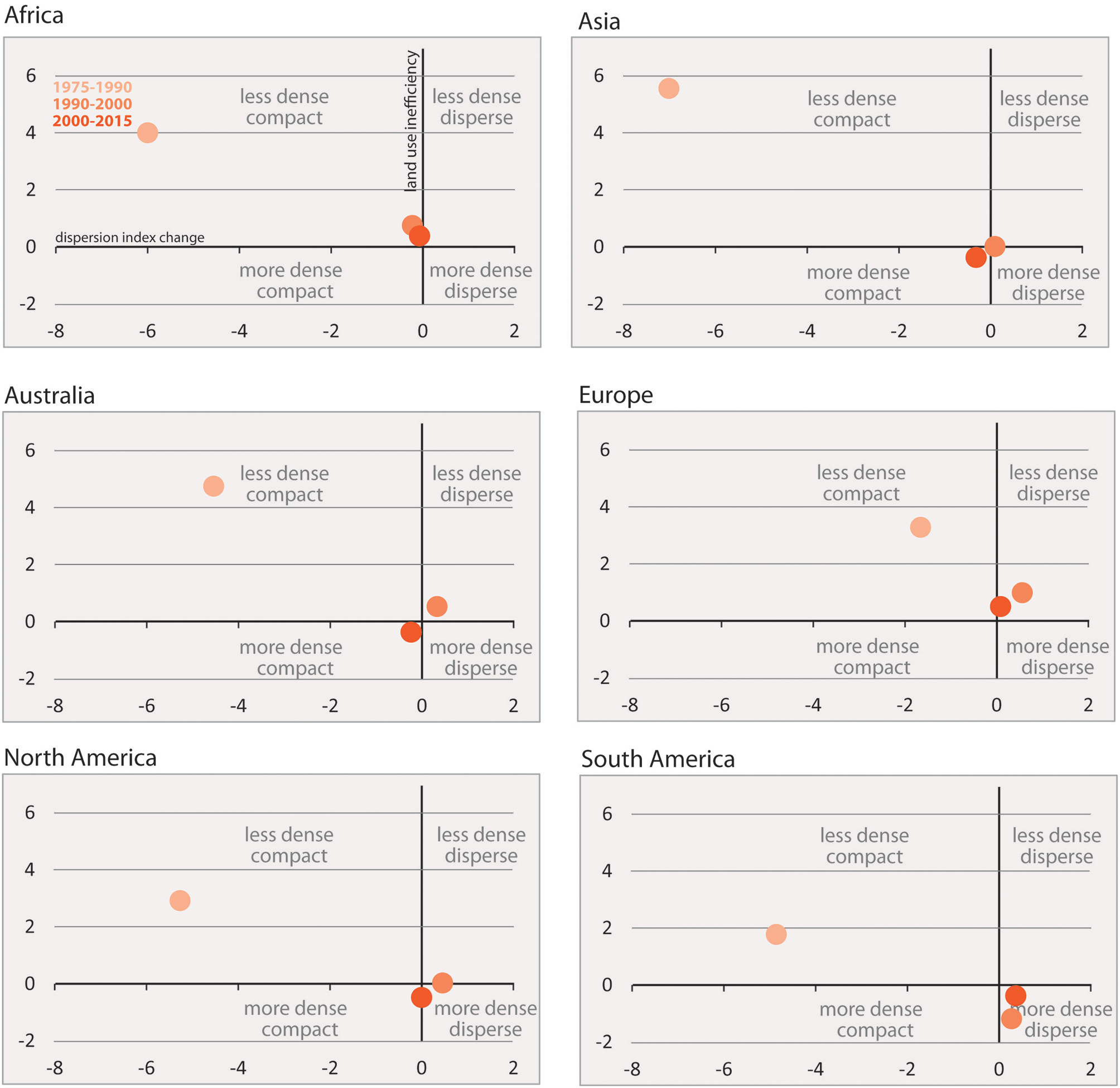
Urbanization trends for the continents.
The above findings are typical for mature urban development with comparatively slow dynamics; however, the results show urban areas steadily becoming less dense and more dispersed due to fewer people on average using and increasing amount of urban land. In North and South America, the growth patterns can be described as becoming denser but dispersed over time, with a slowing dynamic in the most recent observation period from 2000 to 2015. In this context, it would be of great value to enhance this analysis with ring structures, which we demonstrate in further analyses for Paris and Chicago in the next section. The presence of rings around the inner city allows for a differentiation of urban structures from the historical core to the latest phases of urban extensions and for the monitoring of the land use inefficiency and dispersion dimensions for each ring. This analysis could be conducted for all of the cities in the sample if the validity of the measurement concept can further be substantiated in future studies.
For the time being, we would like to highlight that the interpretation of the results presented here follows the movements of points from paler shades of red to the location of the darkest red point. This dark red point symbolizes the end of our observation period. The values very close to the zero point of both axes show a decreasing dynamic that we interpret as a mature level of consolidation for urban development. The analytical value of this observation lies in the future monitoring of these points across the four quadrants. Once policies for urban containment and land saving densification are in place, one can detect progress toward policy objectives using this method.
In order to examine the difference of indicator results between the continents we apply the Kruskal-Wallis-Test (Vargha and Delaney, 1998) to all city regions in the sample, grouped by continent. The calculations were done in the SPSS statistical software package. Complete tables for the summary results presented here can be found in Supplementary Tables 5–24. If the value of the asymptotic significance p of the test is <0.05, there is a difference in the central tendency, otherwise the sample is homogenous. We computed these numbers for the various time periods and the two indicators. If there is indeed a difference, a post-hoc-test determines which continents exhibit significantly different values. In such cases we use the Dunn-Bonferroni-Test df (Cohen, 1992; Dinno, 2015). The results are presented in Tables 3, 4, including the Qui-Square values as context information.
Table 3
| 1975–1990 | 1990–2000 | 2000–2015 | ||||
|---|---|---|---|---|---|---|
| Land use inefficiency | Dispersion index change | Land use inefficiency | Dispersion index change | Land use inefficiency | Dispersion index change | |
| Qui-square | 17,566 | 32,185 | 41,513 | 2,223 | 29,345 | 2,149 |
| Dunn-bonferroni-test (df) | 5 | 5 | 5 | 5 | 5 | 5 |
| Asymptotic significance (p) | 0.004 | 0.000 | 0.000 | 0.817 | 0.000 | 0.828 |
Results of the Kruskal-Wallis-test (continents).
Table 4
| 1975–1990 | 1990–2000 | 2000–2015 | ||||
|---|---|---|---|---|---|---|
| Land use inefficiency | Dispersion index change | Land use inefficiency | Dispersion index change | Land use inefficiency | Dispersion index change | |
| Qui-square | 22,873 | 4,245 | 29,605 | 5,759 | 28,131 | 14,173 |
| Dunn-bonferroni-test (df) | 2 | 2 | 2 | 2 | 2 | 2 |
| Asymptotic significance (p) | 0.000 | 0.120 | 0.000 | 0.056 | 0.000 | 0.001 |
Results of the Kruskal-Wallis-test (city-size).
In the first time period the values for both indicators in the sample are not significantly related, the urban development paths are therefore heterogeneous. The pairwise comparison in the post-hoc-test shows that this result is mainly due to the large difference between urban development paths of South America in comparison to Asian city regions. The medium effect size of r = 0.45 shows that the land use inefficiency deviates significantly, the data shows that it is Asian cities that densify over time, South American cities much less. The heterogeneity of the dispersion index change can mainly be attributed to the difference between Asia and Europe (r = 0.32, medium effect size) and Asia and Africa (r = 0.32, medium effect size). In contrast, the continents in the subsequent periods are homogenous with regards to the dispersion index change. For the land use inefficiency we can also identify differences in the central tendency in the more recent observation periods. For 1990–2000, we see a multitude of relations that emphasize the inequality of urban development paths across continents. The effect size is small and varies between 0.23 and 0.29. In the last period the inequality can mainly be attributed to the difference between Europe and North America (r = 0.23, small size effect), Europe and South America (r = 0.29, small size effect) as well as Europe and Asia (r = 0.21, small size effect).
In addition, we can aggregate the data on the city size level with the same methodology as above. Figure 5 presents the results for the three city categories A, B, and C. The results are similar to the comparison by continent. From 1975 to 1990, the growth dynamic was higher in the smaller cities. The cities in categories B and C develop in a less dense and compact fashion on average at this point as well as in the succeeding time periods. The largest category, cities over 500,000 inhabitants, moves from the quadrant with less density but a compaction of development (upper left) to the denser but dispersed quadrant on the lower right. We interpret these effects as maturing urban development where urban sprawl in the 1980s was followed by a densification and consolidation of suburban areas in the more recent observation periods.
Figure 5
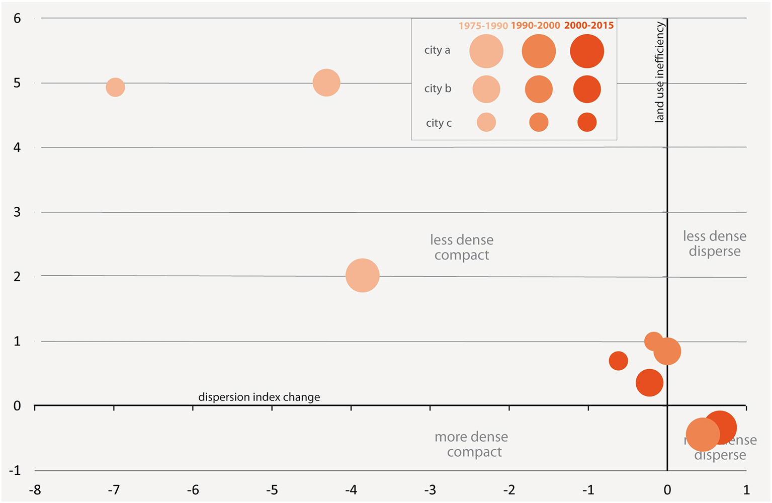
Urbanization trends by city size.
Similar to city region groupings by continent we also conducted the Kruskal-Wallis-Test for city region groupings by city category. For the dispersion index change we identified homogeneity in the sample for the first two decades. However, the asymptotic significance value p for 1990–2000 is close to the level of significance and in the last period it falls under the threshold. This is due to major differences between cities of city category A and the smaller city categories, effect sizes are small. In contrast, we see a continuous heterogeneity between the size classes in terms of land use inefficiency. In all time periods we determine differences in the central tendency between major cities (City A) and the smaller cities (City B and C). Checking for the position of the city size. A symbol in the matrix of Figure 5 which is closer to the x and y axis we can conclude that large cities over 500,000 population have experienced less dispersion and dedensification than smaller cities in the observation period.
Urbanization Trends for Selected Cities
To apply this new methodology for individual cities, we selected Chicago and Paris. Both cities have similar populations (city category A), and they show the largest increase of total urbanized land in their respective countries, the United States of America and France (for more detailed information on city statistics see Supplementary Tables 1, 2). In addition, we can reflect on the urbanization trends for these two cities based on a rich body of literature on their historical development and influential factors (e.g., Dear, 2001; Hudson, 2006; Angel et al., 2010). Such knowledge is valuable in testing new measurement concepts such as the one we present here.
Urbanization Trends in Chicago
With over 2 million inhabitants in the core city and over 9 million in the metropolitan area, Chicago is one of largest cities in the United States. Located at the Western edge of Lake Michigan, Chicago is subject to specific growth conditions that have been a prominent subject of research in urban theory for a long time (Dear, 2001). Waves of suburbanization and reurbanization have changed and enlarged the outskirts of Chicago and have placed pressure on land resources and changes in land rents (McMillen, 2003; Hudson, 2006). To measure the resulting growth patterns since 1975, we have delineated the expansion area toward the west with travel time rings formed as semicircles around the city core, not covering the water area of Lake Michigan. Figure 6 shows that the main areas of rings 1 and 2 were covered by built-up land before 1975. Urban land built between 1975 and 1990 closed the gaps in rings 1 and 2. Urban land extended toward the existing built-up areas in rings 3 and 4. New urban land that was developed after 1990 is mainly located in the outer two rings. Some parts extended new settlement areas in ring 2.
Figure 6
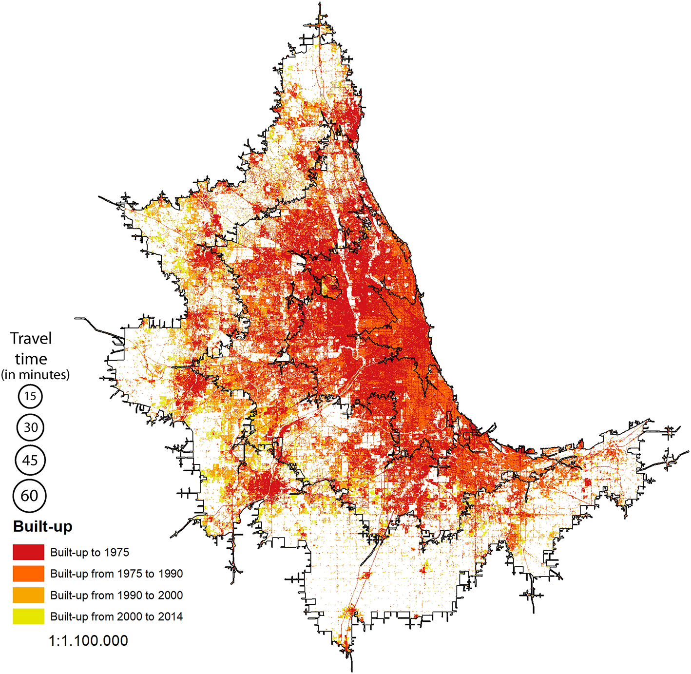
Urbanization periods in Chicago, based on the GHSL.
Figure 7 illustrates urban land use change in Chicago for the three time periods subdivided into the different rings (graphs on the left). To put the values into context, additional graphs on the right show the development of built-up areas (green graph) and population growth (red graph) since 1975. The values are indexed and normalized for the starting value in 1975, which is set to 80. Subsequent developments show the deviation from 80 for the different years after 1975 on the x-axis. This information is complemented by the absolute change of the dispersion index (dark yellow graph) from 1975 to 2015. It is important to note that all of the values represented here are calculated as change rates based on the starting point in 1975.
Figure 7
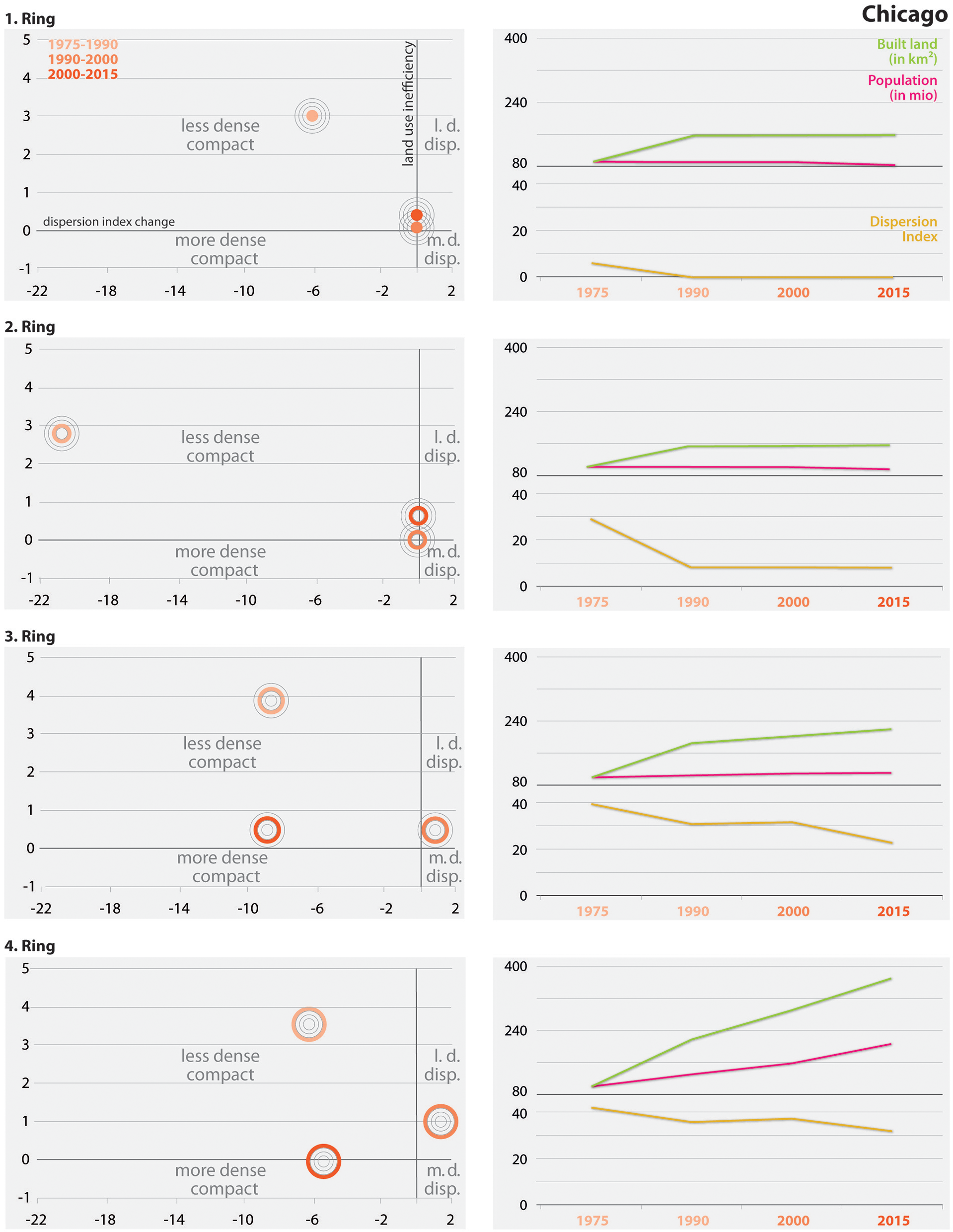
Urbanization trends for Chicago divided into the four rings. The line charts illustrate the corresponding development of built-up land, population, and dispersion index over time.
The resulting graphs on the left-hand side show that the inner core ring represents high growth dynamics in the first time period from 1975 to 1990. This trend reflects a compaction of urban form with a loss of urban density and can be seen as a consequence of the strong suburbanization in this time period during which large shares of the affluent population fled the inner city problems of industrial pollution and crime in deprived neighborhoods (also known as “white flight”) (Boustan, 2010; Boustan and Margo, 2013). The following two periods indicate a further consolidation of the built-up area in the first ring with a decreasing value for the dispersion index change. The decrease in population in the city core continued, leading to a less dense settlement structure during the whole research period. Similar trends can be seen in ring 2. From 1975 to 1990, the total built area increased by ~50 %, while we find no significant changes in the population numbers and a strong decrease in the dispersion index change. Development is found to be less dynamic in the following time periods. We can see a form of stagnation from 1990 to 2000 and decreasing urban density in the last time period due to a shrinking population base. The exterior rings 3 and 4 are similar in their development paths.
Overall, we determine an increasing population in these zones, extraordinary growth rates of built-up land that are typical of suburbanization (graphs on the right-hand side) and shrinking dispersion from 1975 to 2015. Here, the development path during the first period was less dense and very compact. This development is a reflection of continued development in formerly dispersed land use patterns that are typical for the outskirts of large cities. In both outer rings, the second time period from 1990 to 2000 shows a temporal increase in dispersion until 2010, probably a result of newly developed built-up land in isolated locations. However, this trend reversal does not continue in the last given period from 2010 to 2015, where we find a decreasing dispersion index and, therefore, a compaction of urban land use patterns. In this sense, the indicator values in Figure 7 suggest a convergence of the urbanized land in the outer rings.
In summary, we can characterize the urbanization in Chicago as a form of urban consolidation with compact development in the inner rings, and a subsequent compaction of dispersed land use patterns in the outer rings. This is a typical form of suburbanization. The example of Chicago lends itself to the application of this new monitoring concept that provides information about dispersion and land use inefficiency for such urban sprawl conditions. The trend analysis for Chicago shows that the growth in urban land was accompanied by a continuous decrease in urban density over all rings in the research area. We attribute this result to a massive migration of the inner city population to the outer rings in the wake of suburbanization, largely surpassed by the tremendous growth of urbanized land in rings 3 and 4.
Urbanization Trends in Paris
In contrast to Chicago, our second test case, the city of Paris, has no substantial topographic or natural restrictions for urban growth around the city. This lack of restrictions is why Paris has equal travel time rings in a radial growth pattern around the city core, with strong concentrations of newly built urban land along the major transport routes into the hinterland. As the capital of France, Paris has historically attracted urban growth with a concentration of government and business functions for centuries, dominating spatial development with strong transportation linkages to second-tier cities in France. It is therefore not surprising that Figure 8 shows the inner rings as already vastly built-up at the beginning of our observation period in 1975. Newer urban growth mainly occurred in the third ring along the main transportation axis. Ring 4 contains some smaller separated settlement areas in 1975, which we identify as formerly self-contained cities that attracted new growth in our observation period. The urban areas that were created after 1990 extend existing settlements, visible here in the orange and yellow patches of new urban land in rings 3 and 4.
Figure 8
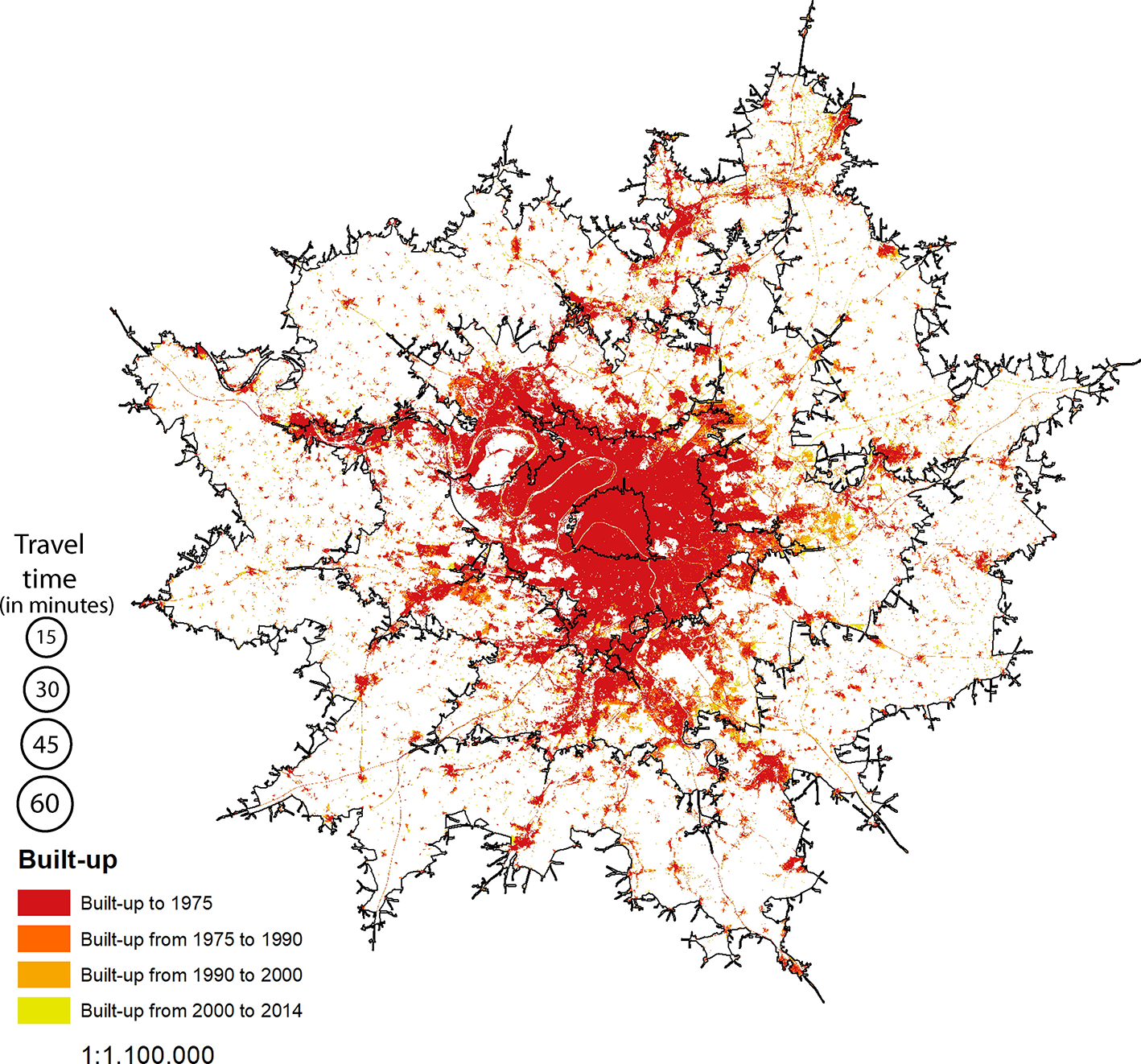
Urbanization periods in Paris, based on the GHSL.
In the city core, the existing urban layout did not allow for much compaction in our observation period; it was already built-up. Our measurement concept reflects this observation accurately: the built-up land and subsequent dispersion remain constant, and the added area of 1.1 km2 of urban land in 39 years of our observation period is marginal considering the area. Nevertheless, we identify continuous population growth in the first ring and therefore a denser settlement structure. The popularity of Paris for city dwellers obviously led to new infill development or perhaps denser forms of living arrangements on average. The second ring, also part of the inner city of Paris, is characterized by dense and compact growth based on the negative land use inefficiency (e.g., population growth exceeding the growth of urban land) and development trends for the dispersion dimension. Figure 9 presents a shift over the time periods from 1975 to 1990, 1990 to 2000, and 2000 to 2015 along the x-axis to the zero point of the dispersion index change dimension.
Figure 9
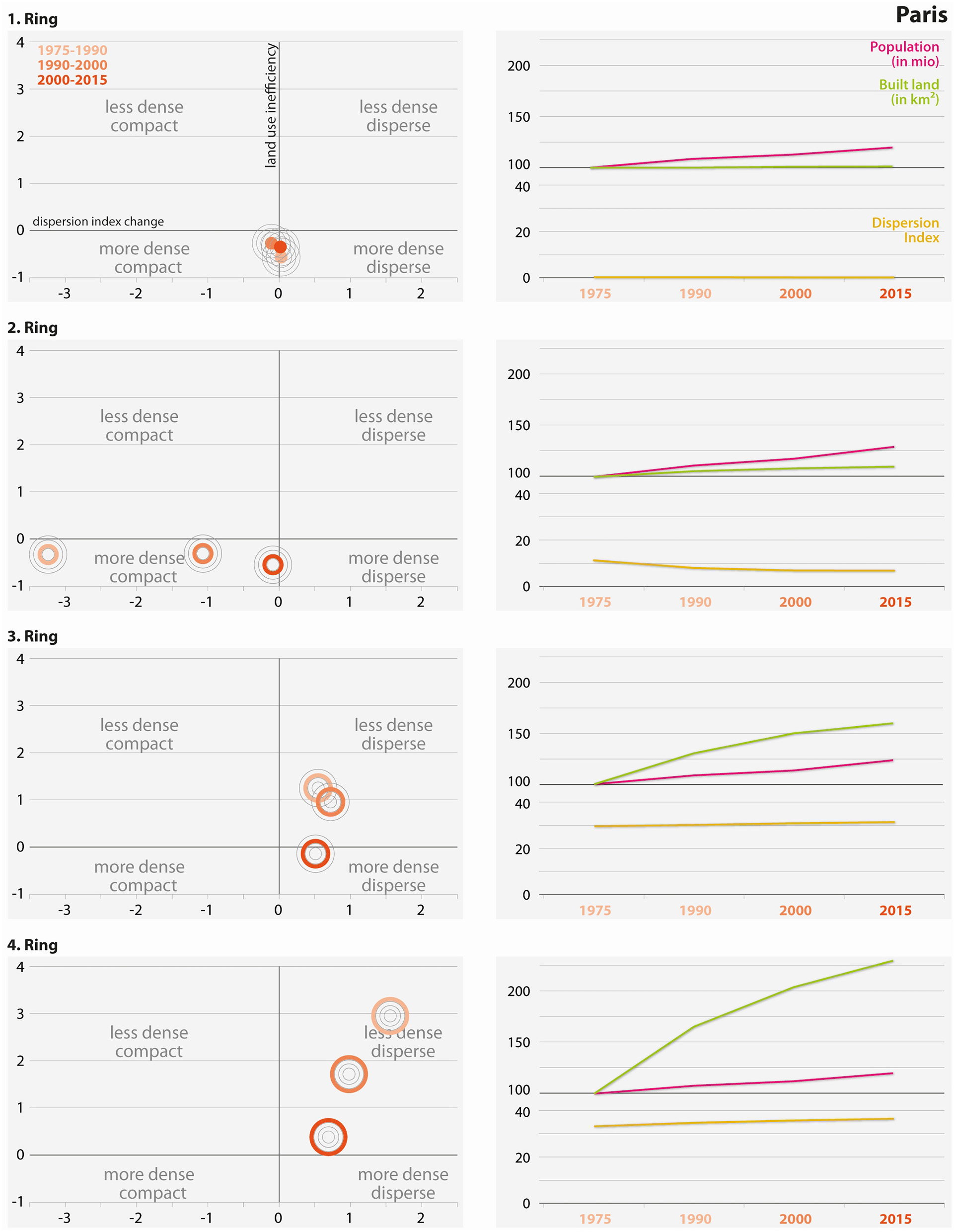
Urbanization trends for Paris divided into the four rings. The line charts illustrate the corresponding development of built-up land, population, and dispersion index over time.
We interpret these changes as a form of spillover effect from the first ring to the second ring where continued population pressure led to a compaction of neighboring suburbs. In contrast to the urban center of Paris, the third ring exhibits a different development path. We can observe increasing values of population and urbanized land but also a growing dispersion in the first two periods. Because we find a higher growth in built-up areas than in population in ring 3, we can assume a form of sprawling suburbanization with less dense and dispersed growth in the first two time periods. However, this trend was reversed in the third time period where population growth exceeds the built-up area growth. The land use inefficiency shows the effect along the y-axis, and the result is a gain of urban density. This minor trend of densification and dispersion in the last period could be a result of densification policies in the city-region (Touati-Morel, 2015). The exterior ring follows this trend with higher dynamics. Notable is the change in the urbanized land, which increases by a factor of 2.5 since 1975 and promotes the dispersion and the decrease in urban density in the fourth ring. We suspect that advantages in land rents and accessibility for commuters shifted the suburbanization from the city core further out to rings 3 and 4 of the research areas. This phenomenon is a typical process for European cities where historically compact cities have seen massive forms of urban sprawl on the outskirts. This is an observation that is often overlooked in theories on urban form that falsely idealize European cities as blueprints for compact city policies (European Environment Agency, 2006).
In summary, in Paris, we can identify different trends from rings 1 through 4. The city core is very compact and can only grow in density; ring 2 experiences a consolidation of urban form as a consequence since 1975. The low value for the dispersion index change in 2015 suggests that this process is largely completed, and the urban form is fully built-up. The developments in rings 3 and 4 have been subject to massive processes of suburbanization and urban sprawl in our observation period, with less dense and disperse growth of urban land and very high land consumption rates.
Discussion
The main results of our study inform about global urbanization trends and new monitoring methods based on remote sensing data. In terms of selected examples on urbanization we show that the highest growth dynamics occurred in the period from 1975 to 1990. In most world regions, this result is typical for the expansive building policies in the wake of the automobile-oriented suburbanization that dominated urban development from the 1950s onward for some decades. This trend is global, although with variations in timing and scale (MacLean, 2008). Our results deliver additional evidence for such variations for selected cities and city groupings in this time period. In the following periods, from 1990 onwards, we see a general compaction of urban development. We attribute this compaction to a consolidation of suburban developments over time with new built-up areas. However, the results of densification or land use inefficiency are not as clear. Most of the cities in our sample show densification in the inner rings and later in the outer rings. Generally, cities exhibit a time lag between the growth of built-up areas and the influx of inhabitants that leads to higher densities. The dichotomy between urban and rural areas becomes blurry.
The additional results of our analysis indicate the following urbanization patterns in the study areas:
Chicago shows a decreasing density that is in line with the results obtained by Angel et al. (2010) from the early 1950s onwards. According to the results of that study, the share of urbanized land increased from 1970 to 2000 from 50 to 100%. We can verify this result with the urbanization shown in Figure 7 that illustrates a steadying trend of increasing land consumption per inhabitant.
Due to the historically established high density in the urban core of Paris, the growth of urbanized land occurred in the outer rings, although the inner city is still growing in population. As a typical characteristic of this process, the settlement patterns are most compact in the city core, and they become more dispersed in the outer rings, following the main transport routes. In the outer rings, the settlement density decreases as a consequence of the high land consumption rate, which is typical for urban sprawl.
Angel et al. (2011) already showed that the growth of urbanized areas in European cities had already peaked before 1975. In contrast, cities in Asia, Africa and South America are still experiencing high growth rates, after 1970 and continuing until the last year of data availability in 2015. These trends were also identified by Seto et al. (2011). Figure 4 shows these differences in land use inefficiency and dispersion dimensions. The results of the statistical analysis present a major difference in the dispersion index change between the continents for the first time period. Since 1990 the sample seems to be more equal. In comparison, the differences of the land use inefficiency for the continents are tremendous for the complete observation time.
From a methodological point of view, our findings show that monitoring methods need to be complemented by validation procedures to test for data reliability. Future analysis must work with ground truth data and more in-depth case studies to assess the accuracy of monitoring results. This aspect is important due to doubts about data quality. As explained in the section on data, we cannot rule out that the limited data quality for the 1975 data is responsible for the large deviations of this time period compared to the trends of the whole observation period. This warning especially applies to the population data presented in section Land Use and Population Data. In terms of land use we expect an improvement of data reliability for more recent years based on the introduction of higher quality sensors and classification procedures. Due to our city selection procedure, our interpretation results on the global level refer only to growing cities. Therefore, we cannot comment on shrinking or stagnating cities. Other methodological findings are:
The differentiation of growth trends according to city size is affected by the cities' catchment areas. For cities with more than 500,000 inhabitants, we used a 45 min travel time polygon as the research unit, which may also include suburban and rural areas in cities with a high density gradient. This area is mostly where urban sprawl happens, namely, at the outskirts along motorways, often as a result of suburbanization processes. In these cities, the urban density can increase in the core. On the outskirts, the urban patterns become more sprawled due to newly developed settlement structures. This effect is evidenced by major differences in land use inefficiency and dispersion between city size categories. Statistical analysis shows that large cities with more than 500,000 inhabitants have consolidated dispersed and inefficient sprawling conditions much more over time than smaller sized cities.
Our analysis of cities by continent does not obtain clear differences for interpretation. Grouping cities by continent obviously mixes too many specific city types with unique development paths, and the resulting average values disguise the analytical power of a single portrayal of development trends such as those we presented for Chicago and Paris. To extract more analytical value from city classes, we aim to concentrate on planning regimes and other characteristic properties of cities for future groupings and the inclusion of different rings of observation.
In essence, we used this study to test a new methodology for a rich database. Our initial results show that the results can be conclusive and reflect global urbanization trends in a new and simplified way. In comparison to other global assessment methodologies (e.g., Seto et al., 2011; Zhang and Seto, 2011) that utilize more measures, we manage to combine the dimensions of population, land expansion, and urban sprawl in one measurement approach. The strength of this methodology is in the analysis of the individual cities and their different catchment areas, which can be adapted for further analysis. Thus, we can assign the development in the individual city rings to different trends of urban land use change. The delineation of cities and their catchments remains a problem for monitoring applications. Our approach to use network analysis and the most recent street network to model multiple rings around an urban core provides the flexibility to analyze urban development phases over time. Based on this approach we can capture land use changes in the rings without relying on the stability of administrative areas. In addition, we do not have to differentiate arbitrarily between urban fringes, suburbia and the rural hinterland, categories that have changed highly dynamically in many city regions of our observation period. In addition, we can customize our methodology. With far-reaching methodological changes of our previous dataset, we are able to exchange the GHSL with similar data sources. The minimum requirements include small-scale information about population and built-up land. Such requirements also apply to our indicators as long as the new indicators are based on the same theoretical and methodological foundations. However, we have also identified limitations in the methodology. To interpret and compare the results additional information such as the initial absolute values of the indicators are useful. Further, our selected indicators also have strengths and weaknesses. As already determined, the application of the dispersion index does not consider the intensity of urban land use or functional centrality (Taubenböck et al., 2018). The indicator focuses on adjacent cells, where minimal inaccuracies in the dataset can break topological adjacency. However, we assess this problem as a minor inaccuracy that is acceptable with a view toward capturing general trends. It is also clear that aspects like urban density could be more accurate when using construction volume or 3D-building data. However, our approach is designed to work with data that is available worldwide, which is not the case for 3D data (e.g., Jahn et al., 2015; Krehl et al., 2016). For future analysis, it would be interesting to compare the results of our simplified analysis to a more complex and detailed measurement. For the time being we can validate the results based on the literature on urban development trends. Future analysis on drivers and impacts will certainly demand additional indicators and qualitative assessments.
We are aware that this idea initially requires some effort to conceptualize. However, once it has been understood and established as a monitoring concept, we expect benefits from its continuous use. In addition, this idea can be a relatively accessible and easy-to-communicate approach for the measurement of urban land use change. The advantage we envisage is that the data requirements are by far not as demanding as in most other measurement concepts. We also expect that further research is needed to make the analytical power more accessible to planning practitioners. Such research must include working with advanced visualization techniques and incorporating other reference data to validate the results. For example, further research could consider planning regimes or economic conditions to obtain information about the development paths of land use change. Such analysis will be left to future endeavors once we have established, communicated, and received feedback on the explanatory value of our methodological approach.
Conclusion
This study was designed to extend measurement methods on urban land use change for worldwide assessments of cities by city size. To achieve this goal, we explored several methods and produced a simplified framework based on the previous studies in Western countries. The idea of this framework is to condense the dimensions of urban land use change suggested in the literature without compromising the analytical depth. Our new approach combines the dimension of urban area, land use patterns, and urban densities into a unified measurement model on two axes: land use inefficiency (built-up area growth divided by population growth) and dispersion of urban patches in the research area.
Overall, the portrayal of global development based on this method provides a first glimpse into the analytical potential of both the method and dataset. Indicator results can be used as single measurements or in the combined analysis of the land use inefficiency and dispersion matrix. Future analysis will provide more insight into the actual development trends by using several rings and other groupings of cities, for example, with a view toward the planning culture or other specific dynamics. For the time being, we introduce this new analytical concept for discussion in the research community. Ideally, we would like to see such analysis used in monitoring applications in planning practice to inform decision makers about urban development paths. Put simply, our recommendation is to capture the starting point of the urban footprint in terms of density and compactness, formulate appropriate objectives, and then begin to monitor development paths with this new method.
The understanding of how cities have grown is an essential facet of the spatial sciences. Newly available, small-scale population and built-up area data serve as the basis for innovative but conceptually challenging analysis options. It is up to the scientific community to improve planner's abilities to effectively employ such data. In this sense, the results presented here deliver on the call of Wei and Ewing (2018) for the development of new monitoring methods for urban land use change.
Statements
Data availability statement
The datasets analyzed for this study can be found in the Global Human Settlement Layer data repository of the European Commission at https://ghsl.jrc.ec.europa.eu/datasets.php (last accessed March 29, 2019). The dataset for the city selection procedure can be found in the world populated places layer package by Esri and Garmin International at https://www.arcgis.com/home/item.html?id=587c838521864164acd245ea03315006 (last accessed August 29, 2019).
Author contributions
CG conducted the analysis and data processing for this paper. The concept and methodology was established by all authors.
Acknowledgments
Jutta Rönsch, cartographer at the Research Institute of Urban Development, assisted in the preparation of Figures 4, 5, 7, 9.
Conflict of interest
The authors declare that the research was conducted in the absence of any commercial or financial relationships that could be construed as a potential conflict of interest.
Supplementary material
The Supplementary Material for this article can be found online at: https://www.frontiersin.org/articles/10.3389/fenvs.2019.00140/full#supplementary-material
Tables with indicator values for Paris and Chicago, excluded countries, list of selected cities per country and the results of the Kruskal-Wallis-Test are provided as Supplementary Material.
Footnotes
1.^See for example the planning tool “Vitalitätscheck” [vitality check] for rural settlements in Bavaria, Germany at http://www.stmelf.bayern.de/landentwicklung/dokumentationen/059178/index.php (March 31, 2019).
References
1
AckermannW.SchweigerM. (2008). F+E-Vorhaben Indikatoren für die nationale Strategie zur biologischen Vielfalt–Bericht zur PAG “Zersiedelungsindikator”. München: PAN Planungsbüro für angewandten Naturschutz GmbH.
2
AdliM. (2017). Stress and the City. Warum Städte uns Krank Machen. Und Warum Sie Trotzdem gut Für uns Sind. München: Bertelsmann Verlag.
3
AngelS.ParentJ.CivcoD. L.BleiA.PotereD. (2011). The dimensions of global urban expansion: Estimates and projections for all countries, 2000–2050. Progr. Plan.75, 53–107. 10.1016/j.progress.2011.04.001
4
AngelS.ParentJ.CivcoD. L.BleiA. M. (2010). The Persistent Decline of Urban Densities: Global and Historical Evidence of Sprawl. Lincoln InstituteWorking Paper. Cambridge, MA: Lincoln Institute of Land Policy. Available online at: http://www.lincolninst.edu/pubs/1834_The-Persistent-Decline-in-Urban-Densities (accessed March 5, 2019).
5
Atlas of Urban Expansion (2019). Available online at: www.atlasofurbanexpansion.org/ (accessed August 15, 2019).
6
BehnischM.KretschmerO.MeinelG. (eds.). (2018). Flächeninanspruchnahme in Deutschland. Auf dem Wege zu einem besseren Verständnis der Siedlungs- und Verkehrsflächenentwicklung. Leibniz-Institut für ökologische Raumentwicklung. Heidelberg: Springer.
7
BoustanL. P. (2010). Was postwar suburbanization “White flight”? Evidence from the black migration. Q. J. Econ.125, 417–443. 10.1162/qjec.2010.125.1.417
8
BoustanL. P.MargoR. A. (2013). A silver lining to white flight? White suburbanization and African–American homeownership, 1940–1980. J. Urban Econ.78, 71–80. 10.1016/j.jue.2013.08.001
9
CalthorpeP.FultonW. (2001). The Regional City. Planning for the End of Sprawl. Washington, DC: Island Press.
10
CerveroR.KockelmanK. (1997). Travel demand and the three ds: density diversity, and design. Transp. Res. D2, 199–219. 10.1016/S1361-9209(97)00009-6
11
CohenJ. (1992). A power primer. Pychol. Bull.112,155–159. 10.1037/0033-2909.112.1.155
12
CouchC.KoeontidouL.Petschel-HeldG. (eds.). (2007). Urban Sprawl in Europe–Landscapes, Land-UseChange & Policy. Oxford: Blackwell Publishing (RICS Research). 10.1002/9780470692066
13
DanielzykR.MünterA.WiechmannT. (eds.). (2016). Polyzentrale Metropolregionen. Cologne: Rohn Verlag.
14
DearM. (2001). From Chicago to LA: Making Sense of Urban Theory.Thousand Oaks, CA: Sage.
15
DinnoA. (2015). Nonparametric pairwise multiple comparisons in independent groups using Dunn's test. Stata J.15, 292–300. 10.1177/1536867X1501500117
16
Esri (2019). ArcGIS-Online – Network analysis coverage. Available online at: https://doc.arcgis.com/en/arcgis-online/reference/network-coverage.htm (accessed August 14, 2019).
17
European Environment Agency (2006). Urban Sprawl in Europe. The Ignored Challenge. EEA Report No 10/2006. Copenhagen: European Environment Agency.
18
European Environment Agency (2011). Landscape Fragmentation in Europe. Joint EEA-FOEN report Copenhagen 9292132156, EEA Report No 2/2011. European Environment Agency.
19
European Environment Agency (2015). The Euroepan Environment. State and Outlook 2015. Synthesis Report. Copenhagen: European Environment Agency.
20
Eurostat (2013). Territorial Typologies for European Cities and Metropolitan Regions. Available online at: https://ec.europa.eu/eurostat/statistics-explained/index.php?title=Territorial_typologies_for_European_cities_and_metropolitan_regions#Functional_urban_areas:_a_city_and_its_commuting_zone (accessed August 14, 2019).
21
Eurostat (2016). Urban Europe. Statistics on Cities, Towns and Suburbs. Edited by European Commission. Luxembourg. Available online at: http://ec.europa.eu/eurostat/web/products-statistical-books/-/KS-01-16-691 (accessed March 29, 2019).
22
Eurostat (2019). Mean Duration of Commuting Time One-Way Between Work and Home by Sex and Age. Available online at: https://appsso.eurostat.ec.europa.eu/nui/show.do?dataset=qoe_ewcs_3c3&lang=en (accessed August 14, 2019).
23
EwingR.RongF. (2008). The impact of urban form on U.S. residential energy use. Hous. Policy Debate19, 1–30. 10.1080/10511482.2008.9521624
24
FinaS. (2013). Indikatoren der Raumentwicklung. Flächeninanspruchnahme und Landschaftszersiedelung. Tübingen: Eberhard Karls Universität Tübingen; Geographisches Institut.
25
FinaS.OsterhageF.RönschJ.RuscheK.SiedentopS.VolgmannK.et al. (2019). Monitoring stadtregionen–neue suburbanisierungsprozesse, in Housing and Housing Politics in European Metropolises, eds WehrhahnR.HannemannC.OthengraphenF.PohlanJ.Schmidt-LauberB. (Leverkusen: Verlag Barbara Budrich).
26
FlorczykA. J.CorbaneC.SchiavinaM.PesaresiM.MaffeniniL.MelchiorriM.et al. (2019). GHS Urban Centre Database 2015, Multitemporal and Multidimensional Attributes, R2019A. Brussels: European Commission; Joint Research Centre (JRC).
27
FregolentL.ToninS. (eds.). (2015). Growing Compact. 1 Band: FRANCOANGELI/Urbanistica. Milan: Franco Angeli Edizioni.
28
FreireS.MacManusK.PesaresiM.Doxsey-WhitfieldE.MillsJ. (2016). Development of New Open and fRee Multi-temporal Global Population Grids at 250 m Resolution. Available online at: https://agile-online.org/conference_paper/cds/agile_2016/shortpapers/152_Paper_in_PDF.pdf (accessed February 5, 2019).
29
FrenkelA.AshkenaziM. (2008). Measuring urban sprawl. How can we deal with it?Environ. Plann. B.35, 1–24. 10.1068/b32155
30
GalsterG.HansonR.WolmanH.ColemanS. (2001). Wrestling sprawl to the ground. Defining and measuring an elusive concept. Hous. Policy Deb. 12, 681–717. 10.1080/10511482.2001.9521426
31
HaaseD.GüneralpB.DahiyaB.BaiX.ElmqvistT. (2018). Global urbanization, in Urban Planet: Knowledge towards Sustainable Cities, eds ElmqvistT.BaiX.FrantzeskakiN.GriffithC.MaddoxD.McPhearsonT.et al. (Cambridge: Cambridge University Press), 19–44.
32
HasseJ. E.LathropR. G. (2003). Land resource impact indicators of urban sprawl. Appl. Geogr.23, 159–175. 10.1016/j.apgeog.2003.08.002
33
HerzigA.NguyenT. T.AusseilA. G. E.MaharjanG. R.DymondJ. R.et al. (2018). Assessing resource-use efficiency of land use. Environ. Model. Softw.107, 34–49. 10.1016/j.envsoft.2018.05.005
34
HudsonJ. (2006). Chicago: A Geography of the City and its Region. Chicago, IL: University of Chicago.
35
HugoG. (2017). New Forms of Urbanization. Beyond the Urban-Rural Dichotomy. London: Routledge.
36
JaegerJ.BertillerR. (2006). Aufgaben und grenzen von messgrössen für die landschaftsstruktur –das beispiel zersiedelung, in Landschaftsqualitäten. Festschrift für Prof. Dr. Klaus C. Ewald, Anlässlich Seiner Emeritierung im Jahr 2006, eds TannerK. M.BürgiM.CochT. (Bern; Stuttgart; Wien: Haupt Verlag), 159–184.
37
JaegerJ.BertillerR.SchwickC.CavensD.KienastF. (2010). Urban permeation of landscapes and sprawl per capita. New measures of urban sprawl. Ecol. Indic.10, 427–441. 10.1016/j.ecolind.2009.07.010
38
JaegerJ.BertillerR.SchwickC.KienastF. (2009). Suitability criteria for measures of urban sprawl. Ecol. Indic.10, 397–406. 10.1016/j.ecolind.2009.07.007
39
JahnA.HechtR.MeinelG. 3D.-Gebäudemodelle (2015). Grundlage siedlungsstruktureller analysen am beispiel sachsens, in Flächennutzungsmonitoring VII: Boden, Flächenmanagement, Analysen und Szenarien, eds MeinelG.SchumacherU.BehnischM.KrügerT. (Berlin: Rhombos-Verlag), 233–243.
40
KeilR. (2017). Suburban Planet. Making the World Urban From the Outside In. Hoboken, NJ: John Wiley & Sons.
41
KrehlA.SiedentopS.TaubenböckH.WurmM. (2016). A comprehensive view on urban spatial structure: urban density patterns of German city regions. Int. J. Geo-Inf.5:76. 10.3390/ijgi5060076
42
Landesanstalt für Umwelt Messungen und Naturschutz Baden-Württemberg. (2007). Indikatoren zur Flächeninanspruchnahme und Flächensparenden Siedlungsentwicklung in Baden-Württemberg. Karlsruhe: Landesanstalt für Umwelt, Messungen und Naturschutz Baden-Württemberg.
43
MacLeanA. (2008). Over. Der American Way of Life oder Das Ende der Landschaft. München: Schirmer/Mosel.
44
McGarigalK. (2015). Fragstats Help. Available online at: https://www.umass.edu/landeco/research/fragstats/documents/fragstats.help.4.2.pdf (accessed January 31, 2019).
45
McGranahanG.BalkD.AndersonB. (2007). The rising tide: assessing the risks of climate change and human settlements in low elevation coastal zones. Environ. Urban.19, 17–37. 10.1177/0956247807076960
46
McMillenD. (2003). Employment subcenters in Chicago: past, present, and future. Econ. Persp.27, 2–14.
47
Organization for Economic Cooperation and Development (2013). Compact City Policies. OECD Green Growth Studies. Paris: OECD
48
PesaresiM.EhrlichD.FerriS.FlorczykA. J.FreireS.HalkiaS.et al. (2016). Operating Procedure for the Production of the Global Human Settlement Layer from Landsat data of the epochs 1975, 1990, 2000, and 2014. EUR 27741 EN, 2016. Brussels: Publications Office of the European Union.
49
PesaresiM.HuadongG.BlaesX.EhrlichD.FerriS.GueguenL.et al. (2013). A global human settlement layer from optical HR/VHR RS data: concept and first results. IEEE J. Sel. Top. Appl. Earth Observ. Remote Sens.6, 2102–2131. 10.1109/JSTARS.2013.2271445
50
SetoK. C.FragkiasM.GüneralpB.ReillyM. K. (2011). A meta-analysis of global urban land expansion. PLoS ONE6:e23777. 10.1371/journal.pone.0023777
51
SiedentopS. (2005). Urban sprawl–verstehen, messen, steuern. DISP160, 23–35. 10.1080/02513625.2005.10556903
52
SiedentopS.FinaS. (2010). Monitoring urban sprawl in Germany towards a GIS-based measurement and assessment approach. J. Land Use Sci. 5, 73–104. 10.1080/1747423X.2010.481075
53
SouleD. C. (2006). Urban Sprawl. A Comprehensive Reference Guide. Santa Barbara, CA: Greenwood Publishing Group.
54
TaubenböckH.WurmM.GeißC.DechS.SiedentopS. (2018). Urbanization between compactness and dispersion: designing a spatial model for measuring 2D binary settlement landscape configurations. Int. J. Dig. Earth12, 1–20. 10.1080/17538947.2018.1474957
55
TosicsI.SzemzoH.IllésD.GertheisA.LalenisK.KalergisD. (2010). National Spatial Planning Policies and Governance Typology. Copenhagen (Peri-Urban Land Use Relationships – Strategies And Sustainability Assessment Tools For Urban-Rural Linkages).
56
Touati-MorelA. (2015). Hard and soft densification policies in the Paris city-region. Int. J. Urban Reg. Res.39, 603–612. 10.1111/1468-2427.12195
57
TsaiY. (2005). Quantifying urban form. Compactness versus ‘sprawl'. Urban Stud.42, 141–161. 10.1080/0042098042000309748
58
United Nations (2018). Sustainable Development Goal 11–Make Cities and Human Settlements Inclusive, Safe, Resilient and Sustainable. Available online at: https://sustainabledevelopment.un.org/sdg11 (accessed February 26, 2019).
59
United Nations (2019). World Population Prospects 2019: Highlights. United Nations. Available online at: https://population.un.org/wpp/Publications/Files/WPP2019_Highlights.pdf (accessed August 16, 2019).
60
VarghaA.DelaneyH. (1998). The Kruskal-Wallis test and stochastic homogeneity. J. Educ. Behav. Stat.23, 170–192. 10.3102/10769986023002170
61
WeiY. D.EwingR. (2018). Urban Expansion, Sprawl and Inequality.Amsterdam: Elsevier.
62
WolffM.HaaseD.HaaseA. (2018). Compact or spread? A quantitative spatial model of urban areas in Europe since 1990. PLoS ONE13:192326. 10.1371/journal.pone.0192326
63
WolmanH.GalsterG.HansonR.RatcliffeM.FurdellK.SarzynskiA. (2005). The fundamental challenge in measuring sprawl: which land should be considered?Prof. Geogr.57, 94–105. 10.1111/j.0033-0124.2005.00462.x
64
ZhangQ.SetoC. (2011). Mapping urbanization dynamics at regional and global scales using multi-temporal DMSP/OLS nighttime light data. Remote Sens. Environ. 115, 2320–2329. 10.1016/j.rse.2011.04.032
Summary
Keywords
urban land use change, urban sprawl, density, dispersion, global human settlement
Citation
Gerten C, Fina S and Rusche K (2019) The Sprawling Planet: Simplifying the Measurement of Global Urbanization Trends. Front. Environ. Sci. 7:140. doi: 10.3389/fenvs.2019.00140
Received
09 April 2019
Accepted
10 September 2019
Published
25 September 2019
Volume
7 - 2019
Edited by
Ioan Cristian Ioja, University of Bucharest, Romania
Reviewed by
Simona R. Gradinaru, University of Bucharest, Romania; Michael W. Strohbach, Technische Universitat Braunschweig, Germany; Manuel Wolff, Humboldt University of Berlin, Germany
Updates
Copyright
© 2019 Gerten, Fina and Rusche.
This is an open-access article distributed under the terms of the Creative Commons Attribution License (CC BY). The use, distribution or reproduction in other forums is permitted, provided the original author(s) and the copyright owner(s) are credited and that the original publication in this journal is cited, in accordance with accepted academic practice. No use, distribution or reproduction is permitted which does not comply with these terms.
*Correspondence: Christian Gerten christian.gerten@ils-forschung.de
This article was submitted to Land Use Dynamics, a section of the journal Frontiers in Environmental Science
Disclaimer
All claims expressed in this article are solely those of the authors and do not necessarily represent those of their affiliated organizations, or those of the publisher, the editors and the reviewers. Any product that may be evaluated in this article or claim that may be made by its manufacturer is not guaranteed or endorsed by the publisher.