Efficient gHMC Reconstruction of Contaminant Release History

1. Introduction

An accurate reconstruction of the release history of contaminants in geophysical systems is essential to regulatory and remedial efforts. These efforts rely on measurements of pollutant concentration to identify the sources and/or release history of a pollutant. Unfortunately, available concentration data are typically sparse in both space and time and are corrupted by measurement errors. Source identification and reconstruction of release history are further complicated by both spatial heterogeneity of model parameters and their insufficient characterization, although we do not consider these effects in the present work.

Detailed reviews of the historic developments and state-of-the-art in the field of inverse modeling as related to contaminant source identification are presented in Atmadja and Bagtzoglou (2001b) and Hutchinson et al. (2017). The existing approaches can be subdivided into two broad classes: deterministic and probabilistic. Deterministic approaches include, but are not limited to, Tikhonov regularization of convolution integrals (Liu and Ball, 1999; Ito and Jin, 2015), least-square estimation from analytical approximations (Butcher and Gauthier, 1994), least-square solution of an optimal control problem (Gugat, 2012), the method of quasi-reversibility (Skaggs and Kabala, 1995; Bagtzoglou and Atmadja, 2003), and the backward beam equation method (Atmadja and Bagtzoglou, 2001a; Bagtzoglou and Atmadja, 2003). These approaches provide estimates of the release history from a source of known locations and are not designed for quantifying the uncertainty associated with these estimates. The robustness of these methods is highly sensitive to measurement errors, and their mathematical formulations are often fundamentally ill-posed.

While existing probabilistic approaches, such as random walk particle tracking for the backward transport equation (Bagtzoglou et al., 1992), minimum relative entropy (Woodbury and Ulrych, 1996), and adjoint methods (e.g., Neupauer and Wilson, 1999), alleviate some of these problems, others remain. For example, these and similar methods do not take advantage of the regularizing nature of the measurement noise and, hence, are often ill-posed. Thus, the minimum relative entropy method treats concentration measurements as ensemble averages. Additionally, there are some outstanding issues with quantifying uncertainty (Neupauer et al., 2000) and the inability of many existing approaches to handle more than one observation point (Neupauer and Wilson, 2005).

Finally, most existing approaches to the reconstruction of release history are restricted to linear transport phenomena, that is, transport phenomena for which the transport equation is linear in the concentration, and thus are limited to migration of contaminants that are either conservative (all the references above) or exhibit first-order (linear) reaction rates (Neupauer and Wilson, 2003, 2004). This is because such approaches are based on either Green's functions (Skaggs and Kabala, 1994; Woodbury and Ulrych, 1996; Stanev et al., 2018) or analytically derived adjoint equations (Neupauer and Wilson, 1999, 2005). The use of Kalman filters for source identification (Herrera and Pinder, 2005) is formally limited to linear transport phenomena and Gaussian errors. While both limitations can be relaxed by employing various generalizations of the Kalman filter such as the extended and ensemble Kalman filter (e.g., Xu and Gömez-Hernández, 2016, 2018), these generalizations are known to fail if the nonlinearity is too strong. Bayesian optimization approaches (Pirot et al., 2019), accelerated by the use of Gaussian process models as surrogates, provide a promising alternative to the Kalman filter since they impose no linearity requirements.

Purely statistical approaches to history reconstruction, such as the geostatistical inversion with Bayesian updating (Snodgrass and Kitanidis, 1997) and various machine learning techniques (Vesselinov et al., 2018, 2019), are applicable to nonlinear transport. Since this is achieved by ignoring governing equations, the reconstructed release histories could have non-physical characteristics, including negative concentrations. These problems have been alleviated by introducing additional constraints into an optimization functional and requiring the reconstructed field to be Gaussian (Michalak and Kitanidis, 2003, 2004a). Combining these geostatistical approaches with analytically derived adjoint equations (Michalak and Kitanidis, 2004b; Shlomi and Michalak, 2007) however brings back the linearity requirement.

We present an optimal reconstruction of contaminant release history that fully utilizes all available information and requires neither the linearity of governing transport equations nor the Gaussianity of the underlying fields. In section 2 we formulate the problem of reconstructing the contaminant release history from noisy observations. Section 3 introduces our general computational framework, which is further implemented in section 4 for various examples.

2. Problem Formulation

2.1. Reconstruction of Contaminant Release History

We consider migration of a single chemically active contaminant in a porous medium Ω ⊂ ℝ^d, d ∈ [1, 3]. We assume that reactive transport is adequately described by the advection-dispersion-reaction equation with reaction term R(c):

$\begin{array}{ll}\frac{\partial c}{\partial t}=\nabla ·(\text{D}\nabla c)-\nabla ·(\text{u}c)-R(c)+r(\text{x},t),\text{x}\in \Omega ,t>0,& (1)\end{array}$

together with corresponding boundary conditions. Here c = c(x, t) is the solute concentration at point x and time t, u is the average macroscopic pore velocity, D is the dispersion coefficient tensor, and r(x, t) is the source function. Both the location and duration of the contaminant release, i.e., the source function r(x, t), can be unknown, but only the former source of uncertainty is treated in the computational examples of section 4, that is, we assume that r(x, t) = r(x)δ(0).

Introducing the dimensionless quantities

$\begin{array}{lll}{c}^{\prime }& =& \frac{c}{c_0},x_i^{\prime }=\frac{x_i}{x_0},i\in \left[1,d\right],t^{\prime }=\frac{t}{t_0},{\text{D}}^{\prime }=\text{D}\frac{t_0}{x_0^2},\\ {\text{u}}^{\prime }& =& \text{u}\frac{t_0}{x_0},r^{\prime }=r\frac{t_0}{c_0},\end{array}$

and the normalized reaction term $R^{\prime }=R{t}_0/c_0$, we rewrite (1) in terms of dimensionless quantities,

$\begin{array}{ll}\frac{\partial c^{\prime }}{\partial t^{\prime }}={\nabla }^{\prime }·({\text{D}}^{\prime }{\nabla }^{\prime }{c}^{\prime })-{\nabla }^{\prime }·({\text{u}}^{\prime }{c}^{\prime })-R^{\prime }+r^{\prime }{\text{x}}^{\prime }\in {\Omega }^{\prime },t^{\prime }>0.& (2)\end{array}$

The non-dimensionalization of the reaction term is specific to its functional form. The non-dimensionalization of a particular case employed in this manuscript is discussed in section 4. For all the following discussions we will consider the dimensionless Equation (2) and we will drop the prime notation for denoting dimensionless quantities.

For the remainder of this work we assume that u, D, and the boundary conditions are known, while the source function r(x, t) is unknown. Our goal is to reconstruct the release history r(x, t) from concentration data ${\bar{c}}_{mi}=\bar{c}({\mathbf{\text{x}}}_m,t_i)$ collected at points ${\left\{{\mathbf{\text{x}}}_m\right\}}_{m=1}^M$ at times ${\left\{t_i\right\}}_{i=1}^I$, and for known u, D, and boundary conditions.

Concentration measurements are corrupted by measurement errors. We assume that the measured concentrations ${\bar{c}}_{mi}$ differ from the true concentration by an additive measurement noise, so that

$\begin{array}{ll}{\bar{c}}_{mi}=c({\text{x}}_m,t_i)+{ϵ}_{mi},& (3)\end{array}$

where the errors ϵ_mi are zero-mean Gaussian random variables with covariance 𝔼[ϵ_miϵ_nj] = δ_ijR_mn, where 𝔼[·] is the expectation operator, δ_ij denotes the Kroneker delta function, and the R_mn, m, n ∈ [1, M], are components of the spatial covariance matrix R ∈ ℝ^M×M of measurement errors. This treatment of measurement noise assumes that the measurements are well separated in time to neglect any temporal correlations, but the model can be easily extended to include temporal correlations. We use the additive error model (3) of Woodbury and Ulrych (1996) rather than the multiplicative error model of Skaggs and Kabala (1994) for the purpose of illustration only. Both models have similar effects on the accuracy of history reconstruction (Neupauer et al., 2000) and can be handled by our approach.

In a typical situation, one has prior information (or a belief) about potential sources of contamination (a region Ω_c within the flow domain Ω) and a time period [T_l, T_u] during which the release has occurred. Examples of Ω_c include spatially distributed zones of contamination (e.g., landfills) and a collection of point sources (e.g., localized/small industrial sites or storage facilities), some of which have contributed to contamination. The lower (T_l) and upper (T_u) bounds of the release interval might represent the time when a landfill became operational and the time when contamination has first been detected, respectively. In the absence of prior information about the release occurrence, one can assume a uniform random distribution of the release in [T_l, T_u] × Ω. We allow for an arbitrary number of measurement points and for either discrete or continuous-in-time measurements.

2.2. Likelihood Function

To simplify the exposition, we assume a spatially distributed chemical release at time t = 0 only, i.e., r(x, t) = c(x, 0)δ(t). Given the measurements $\overline{c}({\mathbf{\text{x}}}_m,t_i)$ and the noise model (3), our goal is to determine the likelihood of a given release configuration c(x, 0). Unfortunately, the measurements, generally taken at later times, do not estimate directly the likelihood of a release configuration. Nevertheless, because the transport Equation (2) is deterministic, we can implicitly assess the likelihood of a given release configuration, P[c(x, 0)], from the probability (likelihood) of a given (computed) concentration history c(x, t). This likelihood can be expressed as (Alexander et al., 2005)

$\begin{array}{ll}P\left[c(\text{x},0)\right]~exp\left\{-{\tilde{H}}_{\text{obs}}\left[c(\text{x},t)\right]\right\},& (4)\end{array}$

where ${\tilde{H}}_{\text{obs}}\left[c(\mathbf{\text{x}},t)\right]$ is the so-called “Hamiltonian” or log-likelihood function,

$\begin{array}{ll}{\tilde{H}}_{\text{obs}}\left[c(\text{x},t)\right]=\frac{1}{2}{\displaystyle \sum _{m,n=1,i=1}^{M,I}}{\Delta }_{mi}{({\text{R}}^{-1})}_{mn}{\Delta }_{ni},& (5)\end{array}$

where ${\Delta }_{mi}\equiv c({\mathbf{\text{x}}}_m,t_i)-\bar{c}({\mathbf{\text{x}}}_m,t_i)$, and R is the covariance matrix of measurement errors, as defined in section 2.1. Since (2) uniquely determines the evolution of the solute concentration from its initial state c(x, 0), the Hamiltonian (5) is a nonlinear functional of the initial conditions c(x, 0), i.e., ${\tilde{H}}_{\text{obs}}\left[c(\mathbf{\text{x}},t)\right]=H_{\text{obs}}\left[c(\mathbf{\text{x}},0)\right]$.

This formulation assumes that the measurement errors ϵ_mi are Gaussian and uncorrelated with the state of the system. Other distributions of the measurement noise and the stochasticity of governing equations can be handled as well (Alexander et al., 2005). The Hamiltonian for stochastic systems, which can represent, e.g., uncertain hydraulic conductivity and flow velocity that are treated as random fields, can be reformulated to explicitly include the transport equation (Alexander et al., 2005; Archambeau et al., 2007).

The contribution of highly fluctuating or unphysical initial conditions is reduced by adding a regularization term H_reg[c(x, 0)] to the observation Hamiltonian (5) and replacing the likelihood function (4) with

$\begin{array}{ll}P\left[c(\text{x},0)\right]~exp\left\{-H\left[c(\text{x},0)\right]\right\},& (\mathrm{6a})\end{array}$

where

$\begin{array}{ll}H\left[c(\text{x},0)\right]=H_{\text{obs}}\left[c(\text{x},0)\right]+\gamma H_{\text{reg}}\left[c(\text{x},0)\right],& (\mathrm{6b})\end{array}$

and the weight γ > 0 is a tuning hyperparameter. The regularization term H_reg is equivalent to a Bayesian log-prior distribution on the initial condition. The selection of an appropriate regularization Hamiltonian is particularly important for problems in which the observation Hamiltonian does not specify a proper probability distribution for c(x, 0) due to a lack of measurements. For a one-dimensional source profile, the squared gradient of the initial spatial profile can play the role of the regularization Hamiltonian. In higher dimensions, one can use a thin-plate penalty functional (Wahba, 1990).

A conceptual difference between our approach and maximum likelihood methods is worth emphasizing. Rather than sampling the Gibbs distribution exp{−H[c(x, 0)]}, as we do here, maximum likelihood methods minimize the Hamiltonian (6b) over c(x, 0). While standard maximum likelihood methods determine the mode and variance of the posterior distribution under a Gaussian approximation, the approach described below can be used to determine the mean and higher-order statistics, and it is valid even when the posterior distribution is multi-modal.

3. Monte Carlo Sampling

In principle, one can sample the Gibbs distribution by using Markov-chain Monte Carlo (MCMC) (e.g., Michalak and Kitanidis, 2003). However, quite often, the disadvantage of local MCMC-based methods is their slow convergence. To improve convergence, we apply a Generalized Hybrid Monte Carlo (gHMC), which enables one to efficiently sample release configurations c(x, 0) with probability given by (6a).

3.1. Hybrid Monte Carlo (HMC)

Hybrid Monte Carlo (HMC) refers to a class of methods that combine Hamiltonian molecular dynamics with Metropolis-Hastings Monte Carlo simulations (see Neal, 1993 for an introductory survey). Specifically, a time-discretized integration of the molecular dynamics equations is used to propose a new configuration, which is then accepted or rejected by the standard Metropolis-Hastings Monte Carlo criteria. The change in total energy serves as the acceptance/rejection criteria.

In HMC one treats the log-likelihood function H in (6b) as the configurational Hamiltonian for a system of N “particles,” each of which has unit mass and generalized coordinates q₁, q₂, …, q_N. Each of these generalized positions corresponds to the solute concentration c(x, t) at a space-time point (x, t). In the following, the particle positions correspond to the initial concentration at time t = 0, e.g., q_i = c(x_i, 0), x_i = iL/(N − 1), i = 0, …, N − 1 for a contaminant release over the one-dimensional domain [0, L].

At any given time, the state of the system is completely described by (q, p), where $\mathbf{\text{q}}={\left\{q_i\right\}}_{i=1}^N$ and $\mathbf{\text{p}}={\left\{p_i\right\}}_{i=1}^N$. Here, the momentum of the ith particle, p_i, is dq_i/dτ = p_i, where τ is the fictitious time of the molecular dynamics. The kinetic energy of the system of N particles is given by

$\begin{array}{ll}{H}_K(\text{p})=\frac{1}{2}{\displaystyle \sum _{i=1}^N}{p}_i^2,& (7)\end{array}$

and the total Hamiltonian of the system is

$\begin{array}{ll}Ĥ(\text{q},\text{p})=H(\text{q})+H_K(\text{p}).& (8)\end{array}$

It follows that the Hamiltonian dynamics are given by

$\begin{array}{ll}\frac{\text{d}{q}_i}{\text{d}\tau }=p_i,\frac{\text{d}{p}_i}{\text{d}\tau }=F_i,F_i=-\frac{\partial H}{\partial q_i},& (9)\end{array}$

where F_i is the force acting on the ith particle, that is to be computed from the governing transport equation. During the time interval Δτ, the system evolves from its current state (q, p) to a new state $(\widetilde{\mathbf{\text{q}}},\widetilde{\mathbf{\text{p}}})$, which can be computed by discretizing the Hamiltonian dynamics (9). An example of such a discretization is the standard leapfrog method, which is written as

$\begin{array}{lll}{\tilde{q}}_i=& q_i+\Delta \tau p_i+\frac{\Delta {\tau }^2}{2}F(\text{q})& (\mathrm{10a})\end{array}$

$\begin{array}{lll}{\tilde{p}}_i=& p_i+\frac{\Delta \tau }{2}\left\{F(\text{q})+F(\tilde{\text{q}})\right\},& (\mathrm{10b})\end{array}$

for i = 1, …, N. Multiple leapfrog steps, i.e., multiple applications of Equation (10), can be performed. For the hybrid Monte Carlo method, the number of leapfrog steps S is larger than one. For S = 1 we obtain the Langevin Monte Carlo method (Neal, 1993). This completes the “proposal part” of HMC.

The remaining part of HMC consists of deciding whether to accept or reject the new state $(\widetilde{\mathbf{\text{q}}},\widetilde{\mathbf{\text{p}}})$. This is done by the Metropolis-Hastings sampling strategy, according to which the new state $(\widetilde{\mathbf{\text{q}}},\widetilde{\mathbf{\text{p}}})$ is accepted with probability

$\begin{array}{ll}Q=min\left\{1,exp\{Ĥ(\text{q},\text{p})-Ĥ(\tilde{\text{q}},\tilde{\text{p}})\}\right\}.& (11)\end{array}$

The momenta variables $\widetilde{\mathbf{\text{p}}}$ are resampled after each acceptance/rejection of the position variables according to a Gaussian distribution of independent variables ~ exp(−H_K). The time-marching and acceptance/rejection process represents one step in the Markov chain, and therefore one Monte Carlo sample. It is important to note that the update from (q, p) to $(\widetilde{\mathbf{\text{q}}},\widetilde{\mathbf{\text{p}}})$ does not conserve energy as a result of the time discretization. The extent to which energy is not conserved is controlled by the time step Δτ. Detailed balance is achieved if the configuration obtained after evolving several steps is accepted with probability Q in (11). Thus, the Metropolis step corrects for time discretization errors.

As we have noted before, the method samples from the multivariate target distribution, ~ exp(−Ĥ), by computing a Markov chain. Sampling from this density allows us to estimate the mean state (reconstructed initial configuration) and its variance. Markov chain sampling from the posterior distribution involves a transient phase, in which we start from some initial state and simulate the Markov chain for a period long enough to reach its stationary density, followed by a sampling phase, in which we assume that the Markov chain visits states from this stationary density. If the chain has converged and the sampling phase is long enough to cover the entire posterior distribution, accurate inferences about any quantity of interest are made by computing the sample mean, variance, and other desired statistics (Landau and Binder, 2009).

3.2. Generalized Hybrid Monte Carlo (gHMC)

In many cases, the generalized hybrid Monte Carlo (gHMC) of Toral and Ferreira (1994) can improve the efficiency of standard HMC by means of the nonlocal sampling strategy described in some detail below. For q,p ∈ ℝ^N, gHMC replaces the Hamiltonian dynamics in (9) with a more general formulation,

$\begin{array}{ll}\frac{\text{d}\text{q}}{\text{d}\tau }=\text{A}\text{p},\frac{\text{d}\text{p}}{\text{d}\tau }={\text{A}}^{\top }\text{F},& (12)\end{array}$

where A is a linear operator represented by a ℝ^N×N matrix. The corresponding leapfrog discretization is then given by

$\begin{array}{lll}\text{q}(\delta \tau )& =\text{q}+\delta \tau \text{A}\text{p}+\frac{\delta {\tau }^2}{2}\text{A}{\text{A}}^{\top }\text{F}\left[\text{q}\right],& (\mathrm{13a})\end{array}$

$\begin{array}{lll}\text{p}(\delta \tau )& =\text{p}+{\text{A}}^{\top }\frac{\delta \tau }{2}\left\{\text{F}\left[\text{q}\right]+\text{F}\left[\text{q}(\delta \tau )\right]\right\}.& (\mathrm{13b})\end{array}$

The two formulations, (9) and (12), are identical if A is the identity matrix. The goal is to find a matrix A that leads to a significant reduction of the temporal correlations of the Markov chain without appreciably increasing the cost of the update due to matrix-vector multiplications.

In order to illustrate how the introduction of the matrix A can help to reduce the correlations of the Markov chain, consider the problem with q ∈ ℝ^N and Hamiltonian

$\begin{array}{l}H(\text{q})=\frac{1}{2}{(\text{q}-\mu )}^{\top }{\Sigma }^{-1}(\text{q}-\mu ),\end{array}$

so that the forcing is given by −Σ⁻¹(q − μ). For the case A = I, it can be seen from (13) that the different components q_i are updated at different rates, given by the covariance matrix Σ. For a given δτ, some components would be updated with long steps, while others would be updated with shorter steps.

The disadvantage of such a configuration is that too long of a step for a certain component might increase the total Hamiltonian enough to produce a rejection according to (11). If the rejection rate of the chain is too large, one would have to reduce δτ, which affects all components. The issue of the rejection rate would be addressed, but then some components would be updated with very short steps, increasing their correlation. To solve this issue, one can remove the appearance of Σ altogether by choosing A such that AA^⊤Σ = I. If Σ is a valid covariance matrix, this is trivially accomplished by choosing A as the Cholesky factor of Σ. We therefore refer to A as the “acceleration” matrix.

Unfortunately, in general, the Hamiltonian (6b) for our problem does not have a simple bilinear form for which an appropriate selection of acceleration matrix A can be derived. Nevertheless, it stands to reason that one can build acceleration matrices for more complex systems to partially reduce the correlation of the Markov chain.

4. Numerical Experiments

In this section we illustrate how the framework outlined above can be applied to source identification problems. In the first case we study the implementation of HMC to contaminant transport problems with a nonlinear reaction term for different configurations of observations. In the second case we study a linear advection-dispersion problem and explore possible selections of the gHMC acceleration matrix.

4.1. Discrete in Space, Continuous in Time Measurements

We consider a one-dimensional transport with uniform velocity u and dispersion coefficient D. We employ as the regularization operator the ℓ₂-norm of the gradient of the initial spatial distribution. Furthermore, we assume that the time of the contaminant release is precisely known and we impose no constraints on the total mass of the released contaminant. The measurements are taken continuously over the time interval (0, T) at a subset J of discrete locations in the spatial domain. We assume that the measurement errors are uncorrelated in space and time and have the same variance ${\sigma }_{ϵ}^2$ at every point. This setup represents observations of contaminant breakthrough curves at a number of sampling locations.

The Hamiltonian corresponding to this setup is

$\begin{array}{ll}H=\frac{1}{2{\sigma }_{ϵ}^2}{\displaystyle {\int }_0^T}{\displaystyle {\sum }_{j\in J}}{\left[c({\text{x}}_j,t)-\bar{c}({\text{x}}_j,t)\right]}^2\text{dt}+\gamma {\displaystyle \underset{\Omega }{\int }}|\nabla c(\text{x},0){|}^2\text{d}x.& (14)\end{array}$

It is evaluated, together with its sensitivity with respect to the initial condition, by using a method-of-lines discretization of the concentration field c(x, t). Once the governing equation has been discretized into a system of ordinary differential equations (ODEs), one can compute the sensitivity ∇_qH via the adjoint sensitivity method (Cao et al., 2003; Li and Petzold, 2004). The disadvantage of this approach is that it incurs two levels of numerical error: the integration error of the forward problem, which affects the initial condition of the adjoint problem, and the integration error of the backward problem. If these errors are significant, both the quality of the estimator and the rejection rate of the Markov chain can be compromised. Reducing the error requires one to decrease the time step used for integration in both directions, which would increase the computational cost per leapfrog step.

To partially alleviate this problem, we use a single-step ODE integration scheme for the forward problem and compute the sensitivity of H with respect to the initial condition via multiple applications of the chain rule (Daescu et al., 2000). Let cⁱ (i = 0, …, I) be a vector of discretized states evaluated at time t = iT/I and ${\widetilde{\mathbf{\text{c}}}}^i$ be a vector of the measurements at time t_i in the elements corresponding to the J measurements' locations and zeros in the other elements. Let C be a diagonal matrix with ones on the diagonal elements corresponding to the J subset of measurement locations and zeros in all other locations. We use this notation to rewrite the observation Hamiltonian and the sensitivity as

$\begin{array}{l}{H}_{\text{obs}}(\text{c},\text{q})=\frac{1}{2{\sigma }_{ϵ}^2}\Delta t{\displaystyle \sum _{i=1}^I}{({\text{c}}^i-{\tilde{\text{c}}}^i)}^{\top }\text{C}({\text{c}}^i-{\tilde{\text{c}}}^i),\end{array}$

and

$\begin{array}{l}{\nabla }_{\text{q}}{H}_{\text{obs}}=\frac{1}{{\sigma }_{ϵ}^2}\Delta t{\displaystyle \sum _{i=1}^I}{\left(\frac{\text{d}{\text{c}}^i}{\text{d}}\text{q}\right)}^{\top }\text{C}({\text{c}}^i-{\tilde{\text{c}}}^i),\end{array}$

respectively, where dcⁱ/dq denotes the Jacobian of cⁱ with respect to q. Using the chain rule, the sensitivity ∇_qH_obs can be rewritten as

$\begin{array}{l}{\nabla }_{\text{q}}{H}_{\text{obs}}=\frac{1}{{\sigma }_{ϵ}^2}\Delta t{\left(\frac{\text{d}{\text{c}}^1}{\text{d}\text{q}}\right)}^{\top }\left[\text{C}({\text{c}}^1-{\tilde{\text{c}}}^1)+{\left(\frac{\text{d}{\text{c}}^2}{\text{d}{\text{c}}^1}\right)}^{\top }\left[\text{C}({\text{c}}^2-{\tilde{\text{c}}}^2)+\cdots \right]\right].\end{array}$

This implies that the sensitivities can be evaluated by repeatedly computing products of the form (dcⁱ⁺¹/dcⁱ)^⊤u. If these products can be computed exactly, then this approach provides the exact sensitivity of the (space-time discretized) system, which is useful for problems with costly forward and backward solutions. The disadvantage of this approach is that it is highly application-specific and restricts the selection of ODE solvers to a specific family. Details of the implementation of this discrete sensitivity analysis approach are presented in Appendix.

We test this formulation on a one-dimensional transport problem defined in the domain [0, L], L = 1 with constant velocity u, dispersion coefficient D, and the reaction model (Lichtner and Tartakovsky, 2003)

$\begin{array}{ll}R(c)=2k(c^2-c_{eq}^2),& (15)\end{array}$

corresponding to a nonlinear heterogeneous (precipitation/dissolution) reaction with equilibrium concentration c_eq. Here k denotes the dimensionless kinetic rate constant normalized by porosity, given by $k=\widehat{k}{t}_0{c}_0$, where $\widehat{k}$ is the kinetic rate constant normalized by porosity, with dimensions of inverse concentration times inverse time, and t₀ and c₀ are the time and concentration scales defined in section 2.1. The parameter values are set to D = 1.0, u = 50.0, c_eq = 0.4, and k = 1.0. Boundary conditions are dc/dx = 0 at x = 0, L. The transport equation is discretized employing a finite-volumes scheme consisting of N = 128 cells of uniform size Δx. Concentration measurements are taken at the M = 3 spatial locations x = L/2, x = 3L/4, and x = L over the time period (0, 2.5 × 10⁻²) (Figure 1). The standard deviation of these measurements is set to σ_ϵ = 0.02.

FIGURE 1

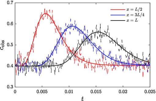
Figure 1. Breakthrough curves of contaminant at observation locations along the transport domain. Noisy measurements used for inference are shown in dashed.

The release configuration is inferred using the HMC scheme, carried out with hybrid timestep Δτ = 0.17, number of leapfrog steps S = 5, and regularizing parameter γ = 0.05. A total of 1 × 10⁵ samples of the release profile were retained after the burn-in period, which are employed to compute the Monte Carlo estimates ${\bar{c}}_0$ and ${\widehat{\sigma }}_{c_0}$ of the posterior mean and standard deviation, respectively. These estimates are shown in Figure 2. In particular, Figure 2A shows the posterior mean estimate ${\bar{c}}_0$ compared to the true release profile, c₀. We also show the 95% confidence interval of the posterior mean estimate. It can be seen that the HMC scheme is able to infer the main features of the initial condition, namely the location of the release and the total mass of contaminant released. For comparison, we also compute the Bayesian maximum a posteriori (MAP) point estimate c_MAP of the release profile, also presented in Figure 2A. The MAP is given by

$\begin{array}{l}{c}_{\text{MAP}}={\displaystyle \underset{c}{arg min}}H\left[c\right],\end{array}$

where H[·] is the Hamiltonian given in (6b). MAP estimation is similar to the method of Bayesian global optimization (BGO) (Pirot et al., 2019) in that both aim to minimize the data misfit. BGO yields an estimate guaranteed to be the global minima over the search space, while MAP may converge toward local minima of the data misfit function. It can be seen that the MAP estimate and the posterior mean estimate are similar, although in general they need not coincide, as they correspond to different statistics. We note that, unlike MAP estimation and Bayesian global optimization, the HMC method is not limited to point estimates and can be used to quantify the uncertainty in the reconstruction. Nevertheless, MAP and Bayesian global optimization estimates are useful when quantifying uncertainty is not critical as their computational cost is smaller than that of HMC.

FIGURE 2

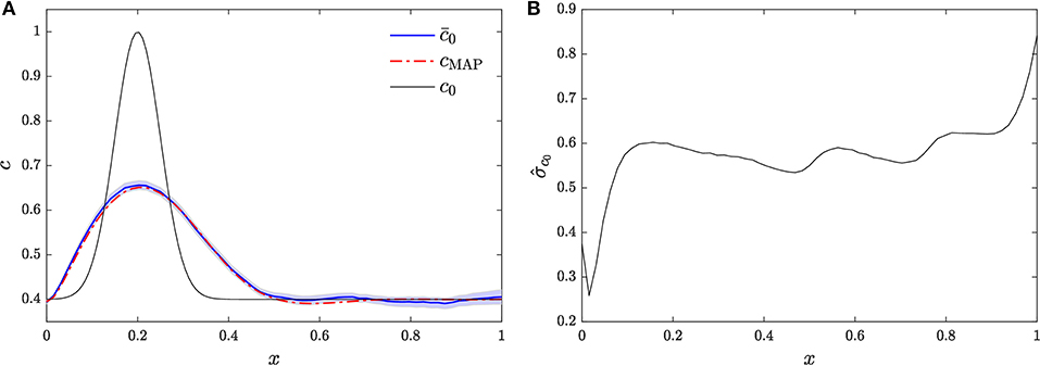
Figure 2. Reconstruction of release profile via HMC. (A) Posterior mean ${\bar{c}}_0$ compared against MAP estimate c_MAP and the actual release profile c₀. (B) Posterior standard deviation.

Figure 2B shows the posterior standard deviation. It can be seen that the posterior standard deviation is large, which is due to the dearth of data available and the ill-posedness of the inversion problem. We also note that the posterior standard deviation is the largest for x = L. Due to the strong advective velocity together with the outflow boundary condition, c₀(L) is only informed by the observations at x = L at early times.

4.2. Application of gHMC to Linear Transport

In order to study the construction of an acceleration matrix A appropriate for contaminant transport, we consider a 1-D advection-dispersion (no reaction) problem

$\begin{array}{ll}\frac{\partial c}{\partial t}+u\frac{\partial c}{\partial x}=D\frac{{\partial }^{2}c}{\partial x^2},x\in \left[0,2\pi \right],t=(0,T],& (16)\end{array}$

with uniform coefficients u and D. This equation is subject to the periodic boundary condition

$\begin{array}{ll}c(0,t)=c(2\pi ,t),& (17)\end{array}$

and (unknown) initial condition

$\begin{array}{ll}c(x,0)=c_0(x).& (18)\end{array}$

Similar to the case studied in section 4.1, available concentration data consist of a set of measurements continuous in time on the interval (0, T) collected at a subset J of the discrete locations x_j, c_{obs, j} = c_obs(x_j, t). The measurements are subject to space-time uncorrelated additive errors of equal variance ${\sigma }_{ϵ}^2$.

4.2.1. Observation Hamiltonian

The state variable c(x, t) is discretized into N functions c_j(t) = c(x_j, t), where x_j = 2πj/N, j = 0, …, N − 1 are N equidistant nodes along the domain [0, 2π). We define the measurement Hamiltonian as

$\begin{array}{ll}{H}_{\text{obs}}=\frac{1}{2{\sigma }_{ϵ}^2}{\displaystyle \sum _{j\in J}}{\displaystyle {\int }_0^T}{\left[c_j(t)-c_{\text{obs},j}(t)\right]}^2\text{dt},& (19)\end{array}$

which defines the likelihood of the measurements given an initial release vector q with components q_j = c_{0, j}. The solution to (16)–(18) can be represented in terms of its discrete Fourier transform (DFT)

$\begin{array}{ll}{ĉ}_k=\frac{1}{N}{\displaystyle \sum _{j=0}^{N-1}}{c}_j{e}^{-ik{x}_j},k=-N/2,\dots N/2-1,& (20)\end{array}$

which defines the N Fourier modes ĉ_k. The backward or inverse transform is given by

$\begin{array}{ll}{c}_j={\displaystyle \sum _{k=-N/2}^{N/2-1}}{ĉ}_k{e}^{ik{x}_j},j=0,\dots ,N-1.& (21)\end{array}$

Let c denote a vector of discrete values c_j and $\widehat{\mathbf{\text{c}}}$ denote its DFT. Then, (20) and (21) can be rewritten as

$\begin{array}{ll}\widehat{\text{c}}=\frac{1}{N}{F}\text{c},\text{c}={{F}}^{*}\widehat{\text{c}},& (22)\end{array}$

where ${F}$ is the DFT matrix whose elements are

$\begin{array}{ll}{{F}}_{pq}={\omega }^{(p-N/2)q},\omega =e^{-2\pi i/N}& (23)\end{array}$

and (·)^* denotes the Hermitian adjoint. By projection, (16) is discretized into the set of uncoupled ODEs for the Fourier modes

$\begin{array}{l}\frac{\partial {ĉ}_k(t)}{\partial t}=-(D{k}^2+iku){ĉ}_k,k=-N/2,\dots N/2-1,\end{array}$

with initial conditions ${ĉ}_k(0)={\widehat{q}}_k$, where the ${\widehat{q}}_k$, k = −N/2, …N/2−1 are the components of $\widehat{\mathbf{\text{q}}}$, the DFT of q ≡ c(0). The solution to the ODEs is then given by

$\begin{array}{ll}{ĉ}_k={\widehat{q}}_{k}exp\left\{-(D{k}^2+iku)t\right\}.& (24)\end{array}$

Substituting (22) and (24) into (19) yields the following expression for the measurement Hamiltonian:

$\begin{array}{l}{H}_{\text{obs}}=\frac{1}{2{\sigma }_{ϵ}^2}{(\widehat{\text{q}}-{\widehat{\text{q}}}_{\text{obs}})}^{*}\left({\displaystyle {\int }_0^T}{\text{B}}^{*}{{F}}_J{{F}}_J^{*}\text{B}\text{d}t\right)(\widehat{\text{q}}-{\widehat{\text{q}}}_{\text{obs}}),\\ =\frac{1}{2{\sigma }_{ϵ}^2}{(\widehat{\text{q}}-{\widehat{\text{q}}}_{\text{obs}})}^{*}{\widehat{\text{G}}}_{\text{obs}}(\widehat{\text{q}}-{\widehat{\text{q}}}_{\text{obs}}),& (25)\end{array}$

where ${\widehat{\mathbf{\text{q}}}}_{\text{obs}}$ is the DFT of c_obs(0), ${{F}}_J$ corresponds to the J columns of ${F}$, B(t) is a diagonal matrix with elements $B_{kk}=exp\left[-(D{k}^2+iku)t\right]$, and ${\widehat{\mathbf{\text{G}}}}_{\text{obs}}$ is a Hermitian (semi)positive definite matrix. The measurement Hamiltonian specifies a multivariate normal distribution for $\widehat{\mathbf{\text{q}}}$, and given that q and $\widehat{\mathbf{\text{q}}}$ are related via a linear transformation, it follows that the measurement Hamiltonian specifies a multivariate normal distribution for q.

If the measurements are available at every node of the computational domain, i.e., if ${{F}}_J={F}$, then ${F}{{F}}^{*}=N\mathbf{\text{I}}$ and (25) simplifies to

$\begin{array}{l}{H}_{\text{obs}}=\frac{N}{2{\sigma }_{ϵ}^2}{(\widehat{\text{q}}-{\widehat{\text{q}}}_{\text{obs}})}^{*}\left({\displaystyle {\int }_0^T}{\text{B}}^{*}\text{B}\text{d}t\right)(\widehat{\text{q}}-{\widehat{\text{q}}}_{\text{obs}}),\end{array}$

which is equivalent to

$\begin{array}{ll}{H}_{\text{obs}}=\frac{N}{2{\sigma }_{ϵ}^2}{\displaystyle \sum _{k=-N/2}^{N/2-1}}|{\widehat{q}}_k-{\widehat{q}}_{\text{obs},k}{|}^2{\widehat{g}}_k& (26)\end{array}$

where the coefficients ĝ_k are given by

$\begin{array}{ll}{\widehat{g}}_k=& {\displaystyle {\int }_0^T}|exp\left\{-(D{k}^2+iku)t\right\}{|}^2\text{d}t\\ =& {\displaystyle \underset{0}{\overset{T}{\int }}}{\text{e}}^{-2D{k}^{2}t}\text{d}t=\frac{1-exp(-2D{k}^{2}T)}{2D{k}^2}.\end{array}$

Note that all coefficients ĝ_k are real, symmetric (ĝ_k = ĝ_−k), and depend only on the dispersion coefficient D.

It follows from (25) that

$\begin{array}{l}{\nabla }_{\text{q}}{H}_{\text{obs}}=\frac{1}{{\sigma }_{ϵ}^2}{{F}}^{*}{\widehat{\text{G}}}_{\text{obs}}(\widehat{\text{q}}-{\widehat{\text{q}}}_{\text{obs}})={{F}}^{*}{\widehat{\text{G}}}_{\text{obs}}{F}(\text{q}-{\text{q}}_{\text{obs}})\\ ={\text{G}}_{\text{obs}}(\text{q}-{\text{q}}_{\text{obs}})\end{array}$

where ${\mathbf{\text{G}}}_{\text{obs}}={{F}}^{*}{\widehat{\mathbf{\text{G}}}}_{\text{obs}}{F}$. That brings the forcing into the form F[q] = −Σ⁻¹(q − μ) required by our analysis in section 3.2, which suggests a possibility of computing the acceleration matrices as $\mathbf{\text{A}}{\mathbf{\text{A}}}^{*}={\mathbf{\text{G}}}_{\text{obs}}^{-1}$. Unfortunately this is not generally feasible, because the matrix G_obs is singular unless the measurements are taken at every node of the domain. The singularity of G_obs implies the singularity of the multivariate normal distribution of $\widehat{\mathbf{\text{q}}}$ given by H_obs, which means the distribution is concentrated in a r-dimensional subspace of ℂ^N, r < N. Since q results from a linear transformation of $\widehat{\mathbf{\text{q}}}$, the multivariate normal distribution of q is also degenerate. This implies that there is a linear subspace of configurations q for which H_obs does not assign a probability, and therefore cannot be identified.

An empirical study of the SVD decomposition ${\widehat{\mathbf{\text{G}}}}_{\text{obs}}=\mathbf{\text{U}}\mathbf{\text{S}}{\mathbf{\text{V}}}^{*}$ of the matrix ${\widehat{\mathbf{\text{G}}}}_{\text{obs}}$ computed for the example of section 4.2.5 provides some insight into features of the degenerate distribution of q defined by the observations. Specifically, the vectors forming a basis for $ker{\widehat{\mathbf{\text{G}}}}_{\text{obs}}$ have negligible terms associated with the lower Fourier modes of q, i.e., |V_{k, j}| ≈ 0 for small |k| and $rank{\widehat{\mathbf{\text{G}}}}_{\text{obs}}<j$. This implies that the lower frequency components of q fall mostly on the subspace of identifiable configurations. In general, |V_{k, j}| ≠ 0 for high |k| and $rank{\widehat{\mathbf{\text{G}}}}_{\text{obs}}<j$, which implies that in general high frequency features cannot be identified.

4.2.2. Regularization Hamiltonian

The regularization Hamiltonian extends the distributions of q and $\widehat{\mathbf{\text{q}}}$ in order to make them well-defined. After a real-space discretization, and accounting for the periodic boundary conditions (17), the ℓ₂-norm regularization Hamiltonian takes the form

$\begin{array}{ll}{H}_{\text{reg}}=\gamma {\text{q}}^{\top }{\text{G}}_{\text{reg}}\text{q},& (27)\end{array}$

where γ is a regularization hyperparameter and G_reg is the circulant matrix

$\begin{array}{l}{\text{G}}_{\text{reg}}=\frac{1}{\Delta x}\left[\begin{array}{ccccc}2& -1& & & -1\\ -1& 2& -1& & \\ & \ddots & \ddots & \ddots & \\ & & -1& 2& -1\\ -1& & & -1& 2\end{array}\right],\end{array}$

or ${\mathbf{\text{G}}}_{\text{reg}}=circ{\left\{\mathbf{\text{r}}\right\}}^{\top }$, where r = (2, −1, 0, …, 0, −1)^⊤/Δx and Δx = 2π/N. The matrix G_reg extends the probability distribution by assigning a high energy (low probability) to configurations with large high-frequency components. To demonstrate this, we rewrite G_reg as

$\begin{array}{l}{\text{G}}_{\text{reg}}=circ{\left\{\text{r}\right\}}^{\top }={\text{F}}^{*}diag\left\{\widehat{\text{r}}\right\}\text{F},{\widehat{r}}_k=\frac{1}{\pi }\left[1-cos\left(\frac{2\pi k}{N}\right)\right],\end{array}$

where $\widehat{\mathbf{\text{r}}}$ is the DFT of r. The components ${\widehat{r}}_k$ of vector $\widehat{\mathbf{\text{r}}}$ increase with frequency k, with the zeroth frequency giving rise to ${\widehat{r}}_0=0$. The latter is to be expected since the regularization operator does not affect the observability of the zeroth frequency, which corresponds to the average of the initial release.

Note that a Fourier-space discretization of the regularization Hamiltonian leads to a similar bilinear form for G_reg, with ${\widehat{r}}_k=2\pi k^2/N^2$. Indeed, these ${\widehat{r}}_k$ have a similar asymptotic behavior as k → 0.

4.2.3. Acceleration Matrix

For the full Hamiltonian H = H_obs+H_reg, the forcing is given by

$\begin{array}{ll}{F}\left[\text{q}\right]=-{\widehat{\text{G}}}_{\text{obs}}(\widehat{\text{q}}-{\widehat{\text{q}}}_{\text{obs}})-{\widehat{\text{G}}}_{\text{reg}}\widehat{\text{q}}=-{\text{G}}_{\text{obs}}(\text{q}-{\text{q}}_{\text{obs}})-{\text{G}}_{\text{reg}}\text{q}& (28)\end{array}$

where ${\text{G}}_{\text{obs}}={{F}}^{*}{\widehat{\mathbf{\text{G}}}}_{\text{obs}}{F}$ and ${\mathbf{\text{G}}}_{\text{reg}}={{F}}^{*}{\widehat{\mathbf{\text{G}}}}_{\text{reg}}{F}$. This suggests that choosing the acceleration matrix A, such that $\mathbf{\text{A}}{\mathbf{\text{A}}}^{*}({\mathbf{\text{G}}}_{\text{obs}}+{\mathbf{\text{G}}}_{\text{reg}})=\mathbf{\text{I}}$, would reduce the correlation of the Markov chain. Since G_obs and G_reg are Hermitian (semi)positive definite, their sum G = G_obs+G_reg is at least Hermitian (semi)positive definite. In fact, G is a full rank matrix and thus can be factorized via a Cholesky decomposition G = S^⊤S. The matrix A, defined by AA^*G =I, is then given by

$\begin{array}{ll}\text{A}={\text{A}}_1={\text{S}}^{-1},{\text{S}}^{\top }\text{S}=\text{G}.& (29)\end{array}$

The added cost of computing the acceleration matrix A is the Cholesky factorization cost, and the leapfrog scheme for gHMC incurs four matrix-vector products. For dense matrices, these costs are ${O}(N^3)$ and ${O}(N^2)$, respectively.

An advantage of the Cholesky factorization is that the vector of momenta p in (13) can be chosen as real and multivariate normal, with zero mean and identity covariance matrix. A drawback is its relatively high cost per step in the Markov chain. Moreover, the matrix G becomes more poorly conditioned as γ → 0, which affects the stability of the Cholesky decomposition.

A less computationally costly alternative for the construction of A is to employ the following heuristic: Instead of using the full correlation matrices in Fourier space, ${\widehat{\mathbf{\text{G}}}}_{\text{obs}}$ and ${\widehat{\mathbf{\text{G}}}}_{\text{reg}}$, to define G, we approximate it as $\mathbf{\text{G}}\approx {{F}}^{*}diag\left\{\overline{\mathbf{\text{g}}}\right\}{F}$, where $\overline{\mathbf{\text{g}}}$ is the vector with components ${ḡ}_i={\left\{{\widehat{\mathbf{\text{G}}}}_{\text{obs}}+{\widehat{\mathbf{\text{G}}}}_{\text{reg}}\right\}}_{ii}$. This approximation allows one to factorize G as $\mathbf{\text{G}}\approx \overline{\mathbf{\text{G}}}={{F}}^{*}\mathbf{\text{D}}{\mathbf{\text{D}}}^{*}{F}$, where $\mathbf{\text{D}}=diag\left\{{(\overline{\mathbf{\text{g}}})}^{1/2}\right\}$ with the square root understood as element-wise. This argument suggests that the acceleration matrix A can be constructed as

$\begin{array}{lll}\text{A}& =& {\text{A}}_2=\frac{1}{N}{{F}}^{*}{\text{D}}^{-1},\text{D}=diag\left\{{(\bar{\text{G}})}^{1/2}\right\},\end{array}$

$\begin{array}{llll}\bar{\text{g}}& =& diag\left\{{\widehat{\text{G}}}_{\text{obs}}+{\widehat{\text{G}}}_{\text{reg}}\right\},& (30)\end{array}$

which gives

$\begin{array}{l}\text{A}\text{p}=\frac{1}{N}({{F}}^{*}{\text{D}}^{-1}\text{p}),{\text{A}}^{*}{F}={\text{D}}^{-1}\left(\frac{1}{N}{F}{F}\right).\end{array}$

Note that we have replaced the transpose of A with its Hermitian transpose due to the complex nature of the DFT. This implies that the transpose in (12) and (13) must be replaced with a Hermitian transpose, and that in order to guarantee that q ∈ ℝ^N we must generalize the momenta such that p ∈ ℂ^N. Once the acceleration matrix A in (30) is constructed, products of the form Ap and A^*F can be computed using DFTs. The computational cost per leapfrog step is reduced from four matrix-vector products of cost $~{O}(N^2)$ to four of cost $~{O}(NlogN)$, and no Cholesky decomposition is necessary.

Since $\overline{\mathbf{\text{g}}}={\partial }^{2}H/\partial {\widehat{\mathbf{\text{q}}}}^2$, the approximation (30) can be thought as building A from the diagonal of the Hessian of H with respect to $\widehat{\mathbf{\text{q}}}$ (a similar heuristic is employed in Neal, 1995 for Bayesian learning). This observation begs the following question: Why do we take $\overline{\mathbf{\text{g}}}={\partial }^{2}H/\partial {\widehat{\mathbf{\text{q}}}}^2$ instead of $\overline{\mathbf{\text{g}}}={\partial }^{2}H/\partial {\mathbf{\text{q}}}^2$, which would produce a similar acceleration matrix A without the Fourier transforms? The answer is that the matrix ${\widehat{\mathbf{\text{G}}}}_{\text{obs}}+{\widehat{\mathbf{\text{G}}}}_{\text{reg}}$ is more concentrated along its diagonal than G is. Hence, more information about the observation operator is conserved by taking the diagonal of ${\widehat{\mathbf{\text{G}}}}_{\text{obs}}+{\widehat{\mathbf{\text{G}}}}_{\text{reg}}$ than the diagonal of G.

4.2.4. Sampling of Momentum Vector

In order to retain the validity of the leapfrog method with generalized momenta, we require said momenta to be associated with a kinetic energy following a bilinear form. We achieve this by assuming that p ∈ ℂ^N has a general complex normal distribution ${C}{N}(0,\Gamma ,\mathbf{\text{C}})$ with unit covariance Γ and

$\begin{array}{ll}\text{C}={\text{A}}^{*}\bar{\text{G}}(conj\text{ A})=\frac{1}{N}\text{D}{F}{{F}}^{\top }{\text{D}}^{-1}.& (31)\end{array}$

For ${{F}}_{pq}$ given by (23),

$\begin{array}{l}\frac{1}{N}{\left({F}{{F}}^{\top }\right)}_{pq}={\displaystyle \sum _{r=0}^{N-1}{\omega }^{r(p+q-N)}}=P_{pq}\\ =\{\begin{array}{ll}1\hfill & \text{ if }p+q=kN,k=\dots ,-1,0,1,\dots ,\hfill \\ 0\hfill & \text{ otherwise}.\hfill \end{array}\end{array}$

where P_pq are the components of the permutation matrix P. Since D is diagonal and P is a permutation matrix (23), yields C = P.

Let p = X + iY with X,Y ∈ ℝ^N. The vector V^⊤ = [X^⊤Y^⊤] is multivariate normal with zero mean. Given Γ and C, the cross-covariance matrix of this vector is

$\begin{array}{l}𝔼\left[\text{X}{\text{Y}}^{\top }\right]=\frac{1}{2}Im\left\{\Gamma +\text{C}\right\}=0,𝔼\left[\text{Y}{\text{X}}^{\top }\right]=\frac{1}{2}Im\left\{-\Gamma +\text{C}\right\}=0,\end{array}$

since both Γ and C are real. In other words, the real and imaginary parts of p are mutually uncorrelated. The covariance matrix of this vector is

$\begin{array}{ll}𝔼[X_i{X}_j]=\frac{1}{2}\mathrm{Re}\{{\Gamma }_{ij}+C_{ij}\}=\{\begin{array}{ll}1\hfill & \text{ if }i=j=0,-N/2\hfill \\ 1/2\hfill & \text{ if }i=-j,i,j\ne 0\hfill \\ 0\hfill & \text{ otherwise},\hfill \end{array}& (\mathrm{32a})\end{array}$

$\begin{array}{ll}𝔼[Y_i{Y}_j]=\frac{1}{2}\mathrm{Re}\{{\Gamma }_{ij}+C_{ij}\}=\{\begin{array}{ll}1/2\hfill & \text{ if }i=-j,i,j\ne 0\hfill \\ 0\hfill & \text{ otherwise}.\hfill \end{array}& (\mathrm{32b})\end{array}$

It follows from (32) that only the components p_k = X_k + iY_k with k = −k are correlated. Their covariances are 𝔼[X_kX_−k] = 0.5, 𝔼[Y_kY_−k] = −0.5. Since p must be complex-symmetric to guarantee that q remains real, we generate p as

$\begin{array}{cc}{X}_{-N/2}~N(0,1),& \\ X_{-N/2+1}~N(0,1/2),& Y_{-N/2+1}~N(0,1/2)\\ ⋮& \\ X_0~N(0,1),& \\ X_1=X_{-1},& Y_1=-Y_{-1},\\ ⋮& \\ X_{N/2-1}=X_{-N/2+1},& Y_{N/2-1}=-Y_{-N/2+1}.\end{array}$

Hence the vector p is generated with N independent identically distributed normal random variables.

4.2.5. Computational Example

We apply the gHMC algorithm to the model problem (16) with parameters D = 1.0, u = 10.0, N = 64, and σ_ϵ = 0.02. Measurements are taken at locations x_j, j ∈ J = {47, 63} over the time period (0, 6 × 10⁻¹). The measurements are shown in Figure 3. To infer the release profile from the observations, we employ A = A₁, S = 5 leapfrog steps, regularization parameter γ = 1 × 10⁻², and hybrid timestep tuned to achieve a rejection rate of 30–35%. A total of 10 chains were generated, each with 2 × 10⁴ samples retained after burn-in. These samples are employed to compute Monte Carlo estimates of the posterior mean and standard deviation, shown in Figure 4.

FIGURE 3

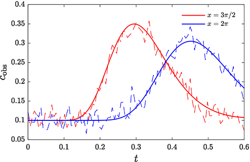
Figure 3. Breakthrough curves of contaminant at observation locations along the transport domain. Noisy measurements used for inference are shown in dashed lines.

FIGURE 4

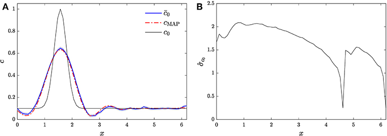
Figure 4. Reconstruction of release profile via gHMC and A = A₁. (A) Posterior mean ${\bar{c}}_0$ compared against MAP estimate c_MAP and the actual release profile c₀. (B) Posterior standard deviation.

Figure 4A compares the posterior mean estimate of the release profile, together with its 95% confidence interval, against the MAP estimate and the true release profile. It can be seen that the gHMC scheme is able to infer the main feature of the release profile. The gHMC estimate also compares favorably to the MAP estimate. Figure 4B shows the posterior standard deviation, which, as in section 4.1, is largely due to the relatively small number of observation locations, the relatively high measurement error, and the ill-posedness of the inverse problem.

Next, we study the effect of the choice of acceleration matrix A on the Markov chains produced by the gHMC algorithm and the Monte Carlo standard error of the posterior mean estimate. Three alternatives for A are considered: A = A₁ in (29), A = A₂ in (30), and A = I (no acceleration). The Monte Carlo standard error is given by $\widehat{\sigma }/\sqrt{n_{\text{eff}}}$, where $\widehat{\sigma }$ is the posterior standard deviation of the inferred parameter, and n_eff denotes the MCMC effective sample size, given by n_eff ≡ n/η (Kass et al., 1998), where n is the number of MCMC samples, and η > 1 is a reduction factor due to the correlation between MCMC samples. This reduction factor is given by

$\begin{array}{l}\eta =1+2{\displaystyle \sum _{s=1}^{\infty }}\rho (s),\end{array}$

where ρ(s) is the autocorrelation of the MCMC chain at lag s. We note that, after convergence, gHMC chains for different choices of A converge to the same posterior mean and standard deviation. The difference of performance between choices of A is in terms of the reduction factor η: Better-performing choices of acceleration matrix result in smaller values of η, so that fewer samples are necessary to achieve a certain target error in the estimation of the posterior mean.

We compute 10 gHMC chains for each choice of A and for two choices of regularization parameter γ, 1 × 10⁻² and 1 × 10⁻³, and employ the samples to compute the autocorrelations ρ(s) and the effective sample size reduction ratios for each q_j, j = 0, …, N − 1, except for j = 47, 63, which are included in the observations. Figure 5 presents the autocorrelations for γ = 1 × 10⁻³ and each choice of A. It can be seen that A = A₁ produces highly uncorrelated chains for each of the q_j studied, A = A₂ produces more correlated chains, and A = I produces the most correlated chains. As expected, A₂ provides a compromise between the low autocorrelation / high expense of the full Cholesky decomposition and the high autocorrelation / low cost of A = I.

FIGURE 5

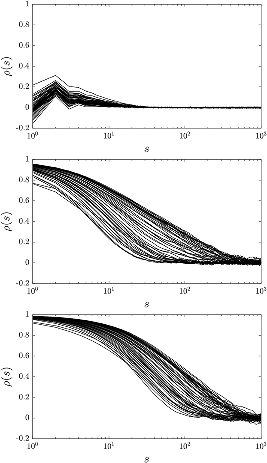
Figure 5. Autocorrelation functions for q_j, j = {0, …, 63}\{47, 63}, and A = A₁ (top), A = A₂ (middle), and A = I (bottom).

The maximum effective sample size reduction ratio η for each choice of A and γ is shown in Table 1. It can be seen that, consistent with Figure 5, A = A₁ produces highly uncorrelated chains, which leads to low values of η, and therefore to smaller standard errors. Similarly, A = I leads to the most correlated chains, the highest values of η, and the highest standard errors, while the choice A = A₂ leads to values of η between those of A = A₁ and A = I. We also note that the values of η for A = A₂ and A = I increase significantly by going from γ = 1 × 10⁻² to γ = 1 × 10⁻³, which is to be expected as the latter is a more challenging case due to weaker regularization. On the other hand, the value of η for A = A₁ does not increase as dramatically when going from γ = 1 × 10⁻² to γ = 1 × 10⁻³, which indicates that A₁ is the best choice of acceleration matrix despite its higher computational cost per leapfrog step. We conclude that the gHMC scheme leads to a significant reduction in the estimation error over the use of HMC without an acceleration matrix.

TABLE 1

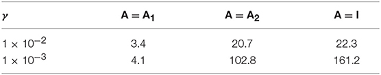
Table 1. Effective sample size reduction ratio η for various choices of regularization parameter γ and acceleration matrix A.

For problems with reaction terms, the forcing F = −∇_qH is not a linear function of q as in (28). In such cases, the selection of the acceleration matrix A is not straightforward. The challenge is to find an approximation to the forcing that is linear in q, i.e., preserves the form (28) with G_obs and G_reg independent of q. This is required to guarantee the reversibility of the Hamiltonian dynamics.

Such an approximation can be obtained by disregarding the nonlinear reaction term and using G_obs in (25) and G_reg in (27), which are functions only of the temporal and spatial domain properties and the hyperparameters ${\sigma }_{ϵ}^2$ and γ. This selection is equivalent to taking F ≈ −G_lin(q − q_obs), where G_lin is the Hessian of the advection-diffusion (linear) portion of the Hamiltonian. It gives the acceleration matrix A₁ of (29). This choice is justified for non-periodic boundary conditions if the contaminant plume does not reach the domain's boundaries during the simulation time. An alternative is to take only the diagonal portion of the Hessian of an advection-diffusion portion of the Hamiltonian. This would produce the acceleration matrix A₂ in (30).

5. Conclusions and Further Work

We presented a computationally efficient and accurate algorithm for identification of sources and release histories of (geo)chemically active solutes. The algorithm is based on a generalized hybrid Monte Carlo approach, in which MC sampling is accelerated by the use of discrete adjoint equations. Some of the salient features of our approach are: (1) its ability to handle nonlinear systems, since it requires no linearizations, and (2) its compatibility with various regularization strategies.

The introduction of an acceleration matrix to the gHMC scheme was tested for an advection-dispersion problem. While the example presented was limited to one-dimensional domains, periodic boundary conditions, and homogeneous porous media, our analysis demonstrated that the proposed acceleration matrices improve upon basic HMC; therefore, we consider the proposed acceleration strategy to be promising. The generalization of these constructions to problems with nonlinear reaction terms, two- and three-dimensional, heterogeneous media, and non-periodic boundary conditions, will be the subject of future work.

Finally, we note the importance of considering the heterogeneity of flow and transport parameters, such as the hydraulic conductivity and dispersion coefficient tensors, for source identification tasks (Xu and Gömez-Hernández, 2018). Attempting to perform Bayesian inference when the values of these coefficients are assumed to be known but their values are erroneous may lead to model misspecification and consequently to posterior densities with little predictive value. Fortunately, the HMC and gHMC schemes presented in this work can accommodate the simultaneous identification of heterogeneous coefficients together with the release history by extending the state vector q to include the discretized heterogeneous coefficients. The calculation of the gradient of the data misfit with respect to the extended state vector can be accomplished via discrete adjoint sensitivity analysis (Zhang et al., 2017) for complex dynamical systems. The extension of the presented framework to the identification of heterogeneous parameters of geophysical models will be considered in future work.

Author Contributions

DB-S implemented the presented algorithms in MATLAB. All authors contributed equally to the preparation of this manuscript.

Funding

This work was supported in part by the Applied Mathematics Program within the U.S. Department of Energy Office of Advanced Scientific Computing Research Mathematical Multifaceted Integrated Capability Centers (MMICCS) project—AEOLUS—Advances in Experimental Design, Optimal Control, and Learning for Uncertain Complex Systems under award number DE-SC0019393, by the U.S. National Science Foundation under award number DMS-1802189, and by the U.S. Department of Energy Office of Basic Energy Research under award number DE-SC0019130. Pacific Northwest National Laboratory is operated by Battelle for the DOE under Contract DE-AC05-76RL01830.

Conflict of Interest

The authors declare that the research was conducted in the absence of any commercial or financial relationships that could be construed as a potential conflict of interest.

The handling editor is currently co-organizing a Research Topic with one of the authors DT, and confirms the absence of any other collaboration.

Acknowledgments

We thank N. Gulbahce and T. Bewley for fruitful discussions.

References

Alexander, F. J., Eyink, G. L., and Restrepo, J. M. (2005). Accelerated Monte Carlo for optimal estimation of time series. J. Stat. Phys. 119, 1331–1345. doi: 10.1007/s10955-005-3770-1

CrossRef Full Text | Google Scholar

Archambeau, C., Opper, M., Shen, Y., Cornford, D., and Shawe-Taylor, J. (2007). “Variational inference for diffusion processes,” in Advances in Neural Information Processing Systems, Vol. 20, eds J. C. Platt, D. Koller, Y. Singer, and S. Roweis (Boston, MA: MIT Press), 1–8.

Google Scholar

Atmadja, J., and Bagtzoglou, A. C. (2001a). Pollution source identification in heterogeneous porous media. Water Resour. Res. 37, 2113–2125. doi: 10.1029/2001WR000223

CrossRef Full Text | Google Scholar

Atmadja, J., and Bagtzoglou, A. C. (2001b). State of the art report on mathematical methods for groundwater pollution source identification. Environ. Forensics 2, 205–214. doi: 10.1080/15275920127949

CrossRef Full Text | Google Scholar

Bagtzoglou, A. C., and Atmadja, J. (2003). Marching-jury backward beam equation and quasi-reversibility methods for hydrologic inversion: application to contaminant plume spatial distribution recovery. Water Resour. Res. 39. doi: 10.1029/2001WR001021

CrossRef Full Text | Google Scholar

Bagtzoglou, A. C., Dougherty, D. E., and Tompson, A. F. B. (1992). Application of particle methods to reliable identification of groundwater pollution sources. Water Resour. Manage. 6, 15–23. doi: 10.1007/BF00872184

CrossRef Full Text | Google Scholar

Butcher, J. B., and Gauthier, T. D. (1994). Estimation of residual dense NAPL mass by inverse modeling. Ground Water 32, 71–78. doi: 10.1111/j.1745-6584.1994.tb00613.x

CrossRef Full Text | Google Scholar

Cao, Y., Li, S., Petzold, L., and Serban, R. (2003). Adjoint sensitivity analysis for differential-algebraic equations: the adjoint DAE system and its numerical solution. SIAM J. Sci. Comput. 24, 1076–1089. doi: 10.1137/S1064827501380630

CrossRef Full Text | Google Scholar

Daescu, D., Carmichael, G. R., and Sandu, A. (2000). Adjoint implementation of rosenbrock methods applied to variational data assimilation problems. J. Comput. Phys. 165, 496–510. doi: 10.1006/jcph.2000.6622

CrossRef Full Text | Google Scholar

Gugat, M. (2012). Contamination source determination in water distribution networks. SIAM J. Appl. Math. 72, 1772–1791. doi: 10.1137/110859269

CrossRef Full Text | Google Scholar

Herrera, G. S., and Pinder, G. F. (2005). Space-time optimization of groundwater quality sampling networks. Water Resour. Res. 41. doi: 10.1029/2004WR003626

CrossRef Full Text | Google Scholar

Hutchinson, M., Eyink, G. L., and Restrepo, J. M. (2017). A review of source term estimation methods for atmospheric dispersion events using static or mobile sensors. Inf. Fusion 36, 130–148. doi: 10.1016/j.inffus.2016.11.010

CrossRef Full Text | Google Scholar

Ito, K., and Jin, B. (2015). Inverse Problems: Tikhonov Theory and Algorithms, Vol. 22. Series in Applied Mathematics. Singapore: World Scientific.

Google Scholar

Kass, R. E., Carlin, B. P., Gelman, A., and Neal, R. M. (1998). Markov chain Monte Carlo in practice: a roundtable discussion. Am. Stat. 52, 93–100. doi: 10.1080/00031305.1998.10480547

CrossRef Full Text | Google Scholar

Landau, D. P., and Binder, K. (2009). A Guide to Monte Carlo Simulations in Statistical Physics. Cambridge, UK: Cambridge University Press.

Google Scholar

Li, S., and Petzold, L. (2004). Adjoint sensitivity analysis for time-dependent partial differential equations with adaptive mesh refinement. J. Comput. Phys. 198, 310–325. doi: 10.1016/j.jcp.2003.01.001

CrossRef Full Text | Google Scholar

Lichtner, P. C., and Tartakovsky, D. M. (2003). Upscaled effective rate constant for heterogeneous reactions. Stochas. Environ. Res. Risk Assess. 17, 419–429. doi: 10.1007/s00477-003-0163-3

CrossRef Full Text | Google Scholar

Liu, C., and Ball, W. P. (1999). Application of inverse methods to contaminant source identification from aquitard diffusion profiles at Dover AFB, Delaware. Water Resour. Res. 35, 1975–1985. doi: 10.1029/1999WR900092

CrossRef Full Text | Google Scholar

Michalak, A. M., and Kitanidis, P. K. (2003). A method for enforcing parameter nonnegativity in Bayesian inverse problems with an application to contaminant source identification. Water Resour. Res. 39. doi: 10.1029/2002WR001480

CrossRef Full Text | Google Scholar

Michalak, A. M., and Kitanidis, P. K. (2004a). Application of geostatistical inverse modeling to contaminant source identification at Dover AFB, Delaware. J. Hydraul. Res. 42, 9–18. doi: 10.1080/00221680409500042

CrossRef Full Text | Google Scholar

Michalak, A. M., and Kitanidis, P. K. (2004b). Estimation of historical groundwater contaminant distribution using the adjoint state method applied to geostatistical inverse modeling. Water Resour. Res. 40. doi: 10.1029/2004WR003214

CrossRef Full Text | Google Scholar

Neal, R. M. (1993). Probabilistic Inference Using Markov Chain Monte Carlo Methods. Technical Report CRG-TR-93-1, University of Toronto.

Google Scholar

Neal, R. M. (1995). Bayesian learning for neural networks (Ph.D. thesis). University of Toronto, Toronto, ON, Canada.

Google Scholar

Neupauer, R. M., Borchers, B., and Wilson, J. L. (2000). Comparison of inverse methods for reconstructing the release history of a groundwater contamination source. Water Resour. Res. 36, 2469–2475. doi: 10.1029/2000WR900176

CrossRef Full Text | Google Scholar

Neupauer, R. M., and Wilson, J. L. (1999). Adjoint method for obtaining backward-in-time location and travel time probabilities of a conservative groundwater contaminant. Water Resour. Res. 35, 3389–3398. doi: 10.1029/1999WR900190

CrossRef Full Text | Google Scholar

Neupauer, R. M., and Wilson, J. L. (2003). Backward location and travel time probabilities for a decaying contaminant in an aquifer. J. Contam. Hydrol. 66, 39–58. doi: 10.1016/S0169-7722(03)00024-X

CrossRef Full Text | Google Scholar

Neupauer, R. M., and Wilson, J. L. (2004). Forward and backward location probabilities for sorbing solutes in groundwater. Adv. Water Resour. 27, 689–705. doi: 10.1016/j.advwatres.2004.05.003

CrossRef Full Text | Google Scholar

Neupauer, R. M., and Wilson, J. L. (2005). Backward probability model using multiple observations of contamination to identify groundwater contamination sources at the Massachusetts Military Reservation. Water Resour. Res. 41. doi: 10.1029/2003WR002974

CrossRef Full Text | Google Scholar

Pirot, G., Krityakierne, T., Ginsbourger, D., and Renard, P. (2019). Contaminant source localization via Bayesian global optimization. Hydrol. Earth Sys. Sci. 23, 351–369. doi: 10.5194/hess-23-351-2019

CrossRef Full Text | Google Scholar

Shlomi, S., and Michalak, A. M. (2007). A geostatistical framework for incorporating transport information in estimating the distribution of a groundwater contaminant plume. Water Resour. Res. 43. doi: 10.1029/2006WR005121

CrossRef Full Text | Google Scholar

Skaggs, T. H., and Kabala, Z. J. (1994). Recovering the release history of a groundwater contaminant. Water Resour. Res. 30, 71–79. doi: 10.1029/93WR02656

CrossRef Full Text | Google Scholar

Skaggs, T. H., and Kabala, Z. J. (1995). Recovering the history of a groundwater contaminant plume: method of quasi-reversibility. Water Resour. Res. 31, 2669–2673. doi: 10.1029/95WR02383

CrossRef Full Text | Google Scholar

Snodgrass, M. F., and Kitanidis, P. K. (1997). A geostatistical approach to contaminant source identification. Water Resour. Res. 33, 537–546. doi: 10.1029/96WR03753

CrossRef Full Text | Google Scholar

Stanev, V. G., Iliev, F. L., Hansen, S., Vesselinov, V. V., and Alexandrov, B. S. (2018). Identification of release sources in advection-diffusion system by machine learning combined with Green's function inverse method. Appl. Math. Model. 60, 64–76. doi: 10.1016/j.apm.2018.03.006

CrossRef Full Text | Google Scholar

Toral, R., and Ferreira, A. (1994). “A general class of hybrid Monte Carlo methods,” in Proceedings of Physics Computing, Vol. 94, eds R. Gruber and M. Tomasi (New York, NY: EPS), 265–268.

Google Scholar

Verwer, J. G., Spee, E. J., Blom, J. G., and Hundsdorfer, W. (1999). A second-order rosenbrock method applied to photochemical dispersion problems. SIAM J. Sci. Comput. 20, 1456–1480. doi: 10.1137/S1064827597326651

CrossRef Full Text | Google Scholar

Vesselinov, V. V., Alexandrov, B. S., and O'Malley, D. (2018). Contaminant source identification using semi-supervised machine learning. J. Contam. Hydrol. 212, 134–142. doi: 10.1016/j.jconhyd.2017.11.002

CrossRef Full Text | Google Scholar

Vesselinov, V. V., Alexandrov, B. S., and O'Malley, D. (2019). Nonnegative tensor factorization for contaminant source identification. J. Contam. Hydrol. 220, 66–97. doi: 10.1016/j.jconhyd.2018.11.010

CrossRef Full Text | Google Scholar

Wahba, G. (1990). Spline Models for Observational Data, Vol. 59. Philadelphia, PA: Society for Industrial Mathematics (SIAM).

Google Scholar

Woodbury, A. D., and Ulrych, T. J. (1996). Minimum relative entropy inversion: theory and application to recovering the release history of a groundwater contaminant. Water Resour. Res. 32, 2671–2681. doi: 10.1029/95WR03818

CrossRef Full Text | Google Scholar

Xu, T., and Gömez-Hernández, J. J. (2016). Joint identification of contaminant source location, initial release time, and initial solute concentration in an aquifer via ensemble kalman filtering. Water Resour. Res. 52, 6587–6595. doi: 10.1002/2016WR019111

CrossRef Full Text | Google Scholar

Xu, T., and Gömez-Hernández, J. J. (2018). Simultaneous identification of a contaminant source and hydraulic conductivity via the restart normal-score ensemble kalman filter. Adv. Water Resour. 112, 106–123. doi: 10.1016/j.advwatres.2017.12.011

CrossRef Full Text | Google Scholar

Zhang, H., Abhyankar, S., Constantinescu, E., and Anitescu, M. (2017). Discrete adjoint sensitivity analysis of hybrid dynamical systems with switching. IEEE Trans. Circ. Syst. I 64, 1247–1259. doi: 10.1109/TCSI.2017.2651683

CrossRef Full Text | Google Scholar

Appendix

Discrete Sensitivity Analysis

For the problem in section 4.1 we use the linearized Runge-Kutta (Rosenbrock) method ROS2 of Verwer et al. (1999) for time stepping of the forward ODE problem. The advantage of using this method is that it allows for a linear implicit treatment of the dispersion operator and a linearization of the reaction operator, while the advection operator is treated explicitly.

We assume that the advection-dispersion-reaction equation can be discretized into an autonomous system of ODEs

$\begin{array}{l}{\text{c}}_t={F}(\text{c})=({\text{A}}_{\text{D}}+{\text{A}}_{\text{A}})\text{c}-\text{R}(\text{c}),\end{array}$

where c is the state vector, A_D is the discretized linear dispersion operator, A_A is the discretized linear advection operator, and R(c) is the reaction vector. Time stepping is performed via a scheme

$\begin{array}{lll}{\text{c}}^{n+1}& ={\text{c}}^n+(2-b)\Delta t{\text{k}}_1+b\Delta t{\text{k}}_2,& (\mathrm{A1})\end{array}$

$\begin{array}{lll}(\text{I}-\theta \Delta t\text{J}){\text{k}}_1& =\text{f}({\text{c}}^n),& (\mathrm{A2})\end{array}$

$\begin{array}{lll}(\text{I}-\theta \Delta t\text{J}){\text{k}}_2& =\text{f}\left({\text{c}}^n+\frac{1}{2b}\Delta {\text{k}}_1\right)-\frac{1}{b}{\text{k}}_1,& (\mathrm{A3})\end{array}$

where $\mathbf{\text{J}}={\mathbf{\text{f}}}_{\mathbf{\text{c}}}({\mathbf{\text{c}}}^n)$ is the Jacobian of f with respect to the state. The coefficients θ and b are taken for this application as $\theta =1-\sqrt{2}/2$ and b = 1/2, respectively. The left-hand side operators of (A2, A3) are approximated via approximate matrix factorization (AMF) to obtain the split form

$\begin{array}{l}(\text{I}-\theta \Delta t\text{J})\approx (\text{I}-\theta \Delta t{\text{A}}_{\text{D}})(\text{I}+\theta \Delta t{\text{r}}_{\text{c}}({\text{c}}^n)).\end{array}$

The discussion in section 4.1 led us to conclude that it is necessary to compute products of the form (dcⁱ⁺¹/dcⁱ)^⊤u in order to apply the discrete sensitivity technique of Daescu et al. (2000). The formulae for the computation of these products are derived from the time-stepping scheme (A1-A3). In particular, differentiating (A1) with respect to the state and multiplying by a test vector u gives the single-step sensitivity product as

$\begin{array}{l}{\left(\frac{\text{d}{\text{c}}^{n+1}}{\text{d}{\text{c}}^n}\right)}^{\top }\text{u}=\text{u}+\frac{3}{2}\Delta t{\left(\frac{\text{d}{\text{k}}_1^n}{\text{d}{\text{c}}^n}\right)}^{\top }\text{u}+\frac{1}{2}\Delta t{\left(\frac{\text{d}{\text{k}}_2^n}{\text{d}{\text{c}}^n}\right)}^{\top }\text{u}.\end{array}$

The next task is to derive formulas for the Jacobians of the stage derivatives k₁ and k₂. Let M be the AMF-ed left-hand-side matrix of (A2, A3). Differentiating (A2, A3) with respect to the state and multiplying by the test vector u gives the formulae

$\begin{array}{ll}{\left(\frac{\text{d}{\text{k}}_1^n}{\text{d}{\text{c}}^n}\right)}^{\top }\text{u}& =\left[{\text{J}}_0-\left(\frac{\text{d}\text{M}}{\text{d}{\text{c}}^n}{\text{k}}_1^n\right)\right]\text{v},{\text{M}}^{\top }\text{v}=\text{u}\end{array}$

and

$\begin{array}{ll}{\left(\frac{\text{d}{\text{k}}_2^n}{\text{d}{\text{c}}^n}\right)}^{\top }\text{u}& ={\text{J}}_1^{\top }\text{v}+{\left(\frac{\text{d}{\text{k}}_1^{n+1}}{\text{d}{\text{c}}^n}\right)}^{\top }\left(\Delta t{\text{J}}_1-2\text{I}\right)\text{v}-{\left(\frac{\text{d}\text{M}}{\text{d}{\text{c}}^n}{\text{k}}_2^n\right)}^{\top }\text{v},\end{array}$

with ${\mathbf{\text{J}}}_0={\mathbf{\text{f}}}_{\mathbf{\text{c}}}({\mathbf{\text{c}}}^n)$, ${\mathbf{\text{J}}}_1={\mathbf{\text{f}}}_{\mathbf{\text{c}}}({\mathbf{\text{c}}}^n+\Delta t{\mathbf{\text{k}}}_1^n)$.

The computation of the products $(\text{d}\mathbf{\text{M}}/\text{d}{\mathbf{\text{c}}}^n){\mathbf{\text{k}}}_i^n$, i = 1, 2 is highly problem-specific. It depends on the structure of the second-order derivatives of the reaction vector with respect to the state. For the reaction model (15) and a method-of-lines discretization, the Jacobian R_c is diagonal, and so the computation of these products is straightforward. For different reaction models and more sophisticated discretization schemes the computation might be more involved.