Abstract
Groundwater in most urban areas around the globe is often contaminated by toxic substances. Among the various sources of contamination, industries cause the heaviest impact when toxic compounds are released underground, mainly through leaking tanks or pipelines. Some contaminants (typically chlorinated hydrocarbons) tend to persist within the underground and are hard to biodegrade. As a result, substances that leaked decades ago are still impacting groundwater. Milano and its surroundings (Functional Urban Area) is a good example of an area that has been hosting industries of all dimensions for over a century, many of them contributing to groundwater contamination from chlorinated hydrocarbons. While the position of the biggest industrial facilities is well-known, many smaller sources are hard to identify in many cases where direct surveys have not been undertaken. Furthermore, the overlapping effects of big, small, known, and unknown sources of groundwater contamination make it challenging to identify the contribution of each. In order to identify the contribution of several point sources responsible for tetrachloroethylene contamination in public water supply wells, a numerical model (MODFLOW-2005) has been implemented and calibrated using PEST in the northwestern portion of the Milano Functional Urban Area. In contaminant transport modeling, the deterministic approach is still favored over the stochastic approach because of the simplicity of its application. Nevertheless, the latter is considered by the authors as the most suitable for dealing with problems characterized by high uncertainty, such as hydrogeological parameter distributions. Adopting a Null-Space Monte Carlo analysis, 400 different sets of hydraulic conductivity fields were randomly generated of which only 336 were selected using an objective function threshold. Subsequently, particle backtracking was performed for each of the accepted hydraulic conductivity fields, by placing particles in a contaminated well. The number of particle passages is considered as being proportional to the contribution of each unknown point source to the tetrachloroethylene contamination identified in the target well. The study provides a methodology to help public authorities to locate the “more probable than not” area responsible for the tetrachloroethylene contamination detected in groundwater and to focus environmental investigations in specific sectors of Milano.
1. Introduction
In urban areas impacted by historical industrialization, the main problem of groundwater contamination is related to chlorinated hydrocarbons (CHCs) (Menichetti and Doni, 2017; La Vigna et al., 2019). Such contamination is typically associated with point sources (PS) or discrete zones, formerly linked to petrochemical plants, refineries, automotive, dry-cleaning, or metal degreasing operations. However, due to the intense industrial and urban development during the last 60 years, it is very difficult to apply the “Polluter Pay Principle” (PPP) (De Sadeleer, 2014; Schwartz, 2018; Covucci, 2019; Milon, 2019). Pollution plumes pose challenges in terms of characterization of contaminant migration pathways, identification of the source, and the polluter. Due to the high uncertainty linked to the exact position of the source, it is necessary to identify the PS with a stochastic approach in order to apply the “more probable than not” principle. Jurisprudence has frequently highlighted the fact that public authorities must identify the operator liable for damage to the environment caused by pollution (D.Lgs 152/2006, Environmental Ministry of Italy, 2006). Particularly, article 239 recalls principles set out by the EU including the PPP. From Directive 2004/35/EC (2004), there is the stem that supports the obligation of imposing the costs of preventive and remediation measures on the operator whose actions or omissions have caused the environmental damage. In the Lombardy Region (Italy), one of the most urbanized and industrialized areas in Europe, nearly 3,000 potential brownfields are present in the contaminated site regional database (AGISCO, ARPA Lombardia, 2019). In such a context, there are many obstacles for remediation as suggested by Alderuccio et al. (2019) and Barilari et al. (2020). The PPP is quite different in many countries: for example, in China (Zahar, 2018), the PPP has been introduced into environmental law, but it seems to be difficult to apply because of the ownership of the National Government. In Spain, the PPP is mixed to the concept of “pay as you throw” (PAYT), which is the method that most directly relates user charges to contributions to environmental sustainability (Chamizo-González et al., 2018). A number of developing countries have recently extended this principle to make it an obligation of the state to compensate the victims of environmental harm (Luppi et al., 2012). In order to apply in Italy both administrative and penal proceedings, a detailed historical analysis of the activities conducted at a site, in conjunction with the link between substances, materials used in production cycles and relationship with the owner, creates the basis for environmental forensics. The link, always “causal,” requires strong supporting “evidence”; in this sense, the criterion of “more probable than not” can be applied. This is a fundamental step for regional authorities that, without identifying those responsible for contamination, have to take charge of the remediation processes. In order to reconstruct such difficult historical backgrounds in highly urbanized areas (i.e., in the Lombardy Region), new scientific and robust methodologies are required in order to identify the suspected sources of contaminant. Among others, compound-specific isotope analysis (Hunkeler et al., 2008; Shouakar-Stash et al., 2009; Alberti et al., 2017), integral pumping tests (Bauer et al., 2004; Alberti et al., 2011), inverse groundwater modeling (Carrera et al., 2005; Tonkin and Doherty, 2009; Alberti et al., 2018; Moeck et al., 2020), and their combination are the most promising techniques. The modeling methodologies have to take into account uncertainties within an “acceptable level,” which depends on the effects and costs of possible contamination and on the complexity of the hydrogeological systems (Frind and Molson, 2018). Uncertainties are given by heterogeneity in the aquifer units, in the regional flow system, in the recharge, and in the conceptual model setup (Rojas et al., 2008). The classical method to identify sources is particle tracking (PT), which involves flow system simulation modeling combined with advective transport of particles along flow lines. For contamination in highly urbanized areas, where a simple termination point (i.e., end-point) analysis is not feasible due to the multiple unknown source release times, the combination of particle tracking with the Null-Space Monte Carlo approach (PT+NSMC) is able to delineate the contribution of each PS under geological uncertainty associating a probability to each of them. It thus enables the public authorities to focus their investigations and to effectively apply the “Polluter Pay Principle”.
2. Materials and Methods
2.1. Study Area and Hydrogeology
The methodology has been developed within the AMIIGA Project (Interreg Central Europe Grant N. CE32), where inverse transport modeling was one of the tools used to assess the unknown sources in the northwestern part of the Milano Functional Urban Area (FUA). The area of 157 km2 covers 12 municipalities with high urbanization density (about 4,000 inhabitants per km2) and a large presence of industrial sites. The area is historically affected by many chlorinated hydrocarbon plumes originating from the northern outer border of the Milano municipality (Giovanardi, 1979; Segre, 1987; Provincia di Milano, 1992); over the last 40 years, the contamination has migrated into Milano city because of the intake area induced by the water supply wells, which provoked a coalescence of several plumes and causing a deterioration of water quality. The evidence is that many plumes that originated in the early 70s in the vicinity of Milano are still affecting the aquifers that supply water to the Milano aqueduct system due to the presence of secondary sources and the retardation process of transport. Many chloride compounds were commonly used for degreasing processes by metallurgical, chemical, galvanizing, dry cleaning, and other industrial plants. Today, the main solvents observed in the water supply wells are tetrachloroethylene (PCE), trichloroethylene (TCE), and thichloromethane (TCM) whose concentrations exceed the CCT (Contamination Concentration Threshold) of Italian Law (D. Lgs 152/2006, Environmental Ministry of Italy, 2006, D. Lgs 31/2001, Environmental Ministry of Italy, 2001). The problems owing to the presence of these substances in waters are (1) the high risk of carcinogenicity in humans and (2) the measures that water managers have to adopt in order to control and remove organic chlorinated compounds from drinking water.
Figure 1 shows the evolution of PCE contamination from 2000 (a) to 2007 (b) in the water supply wells in Milano (in some wells the detected values are higher than 200 μg/l, as represented by violet and brown circles). Furthermore, the urban texture has significantly changed during the last 15 years [the change in the use of soil (from 2000 to 2015) is provided in the Supplementary Figure 2. Some green areas are becoming industrialized and vice versa. The continuous change of use of soil (Masetti et al., 2008) can be one of the causes affecting the groundwater contamination (Pollicino et al., 2019). It is therefore very difficult to reconstruct the suspected areas and consequently to attribute the responsibility of contamination observed in the water supply wells. The Lombardy Region aquifer classification (Regione Lombardia and ENI Divisione Agip, 2002) considers the presence of four different hydrostratigraphic units named A, B, C, and D (a vertical cross-section is shown in the Supplementary Figure 1) that originated due to the overlay of plio-pleistocenic alluvial sediments that filled the Neogene Po plain fore-deep, reaching a maximum thickness of approximately 500 m (Bini, 1987). The main aquifers affected by the contamination (A and B) have alluvial and glacio-fluvial origins, and they have a high transmissivity. The unconfined Aquifer A, has a sandy-gravel texture, and the underlying semi-confined aquifer (Aquifer B) has a fine sand composition, interrupted by clay lenses that subdivide it in several small aquifers (i.e., multilayered aquifer). The two aquifers are undifferentiated in the northern part of the study area, whereas they are hydraulically separated by a clay layer of about a meter in thickness in the Milano area. The historical piezometric data collected for the two aquifers show that Aquifer A presents a hydraulic head, higher than in Aquifer B, of about 1 to 1.5 m, and there is therefore a natural downwelling of flow from the shallow aquifer where the clay aquitard shows discontinuities. More details about the conceptual model can be found in previous works (Cavallin et al., 1983; Beretta et al., 1992, 2004; Alberti et al., 2016; Colombo et al., 2019).
Figure 1
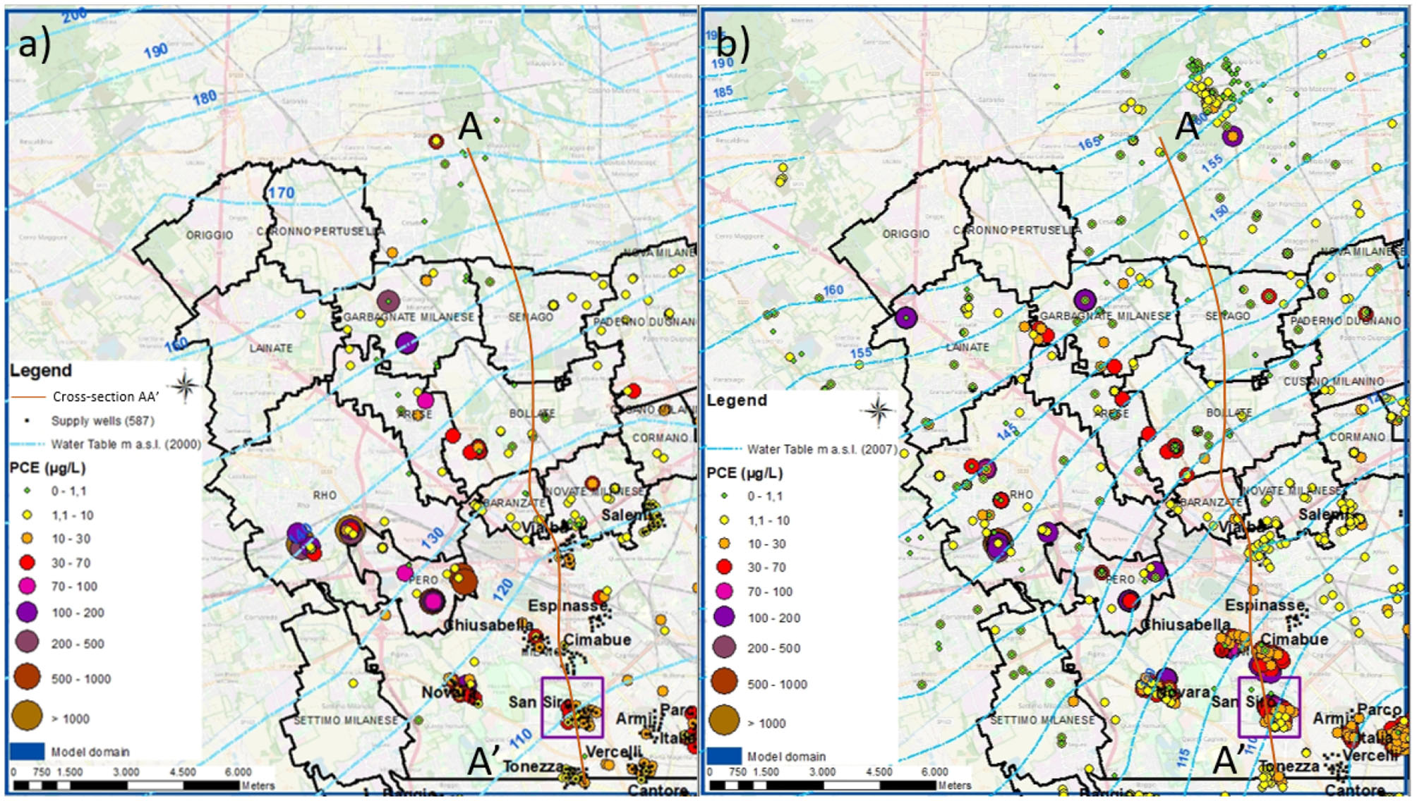
Study area: FUA municipalities with black contours, PCE contamination sampled in (a) 2000 and (b) 2007 with the associated piezometric map. The cross-section AA′ is described in the Supplementary Figure 1.
2.2. Methodology
The model used to carry out the stochastic simulations in this work is briefly described in this section; a more detailed description is provided by Colombo et al. (2019). Nine model layers with variable thickness (Figure 2) are used to represent the two most contaminated geological units (A and B) in the groundwater model (MODFLOW-2005, Harbaugh, 2005), using Groundwater Vistas as the graphical interface (Rumbaugh and Rumbaugh, 2011): Layer 1 represents Aquifer A, layer 2 represents the aquitard, and layers 3–9 represent the so-called multilayered Aquifer B. The model also represents rivers and sinks (i.e., pumping wells), and the horizontal discretization is a 100x100 m grid. Boundary conditions are chosen to be CHs (Constant Heads) and are extrapolated from previous modeling studies (Alberti et al., 2016). The main river (Olona) is implemented as a Cauchy boundary condition. The exchange between superficial water and groundwater is quite low and influences a zone of a few hundred meters around the riverbed. The flow rate depends on the low conductance term defined by hydraulic conductivity and the riverbed thickness (Alberti et al., 2007). An artificial canal used for irrigation purposes is also represented using a Cauchy boundary condition, even if its exchanges with the aquifer are quite low because of its concrete structure. Over the rest of model top, the amount of vertical recharge has been considered uniform in areas with similar land use (divided in urban, agricultural, and green) and estimated through the Thornthwaite method (Thornthwaite, 1948). In the urbanized areas, the contribution of natural recharge is almost null, but a low groundwater recharge is nevertheless assigned in order to consider water network losses (Alberti et al., 2016). More than 750 pumping wells are included in the model (Colombo et al., 2019) of which 200 wells are drinking water wells affected by CHCs contamination.
Figure 2
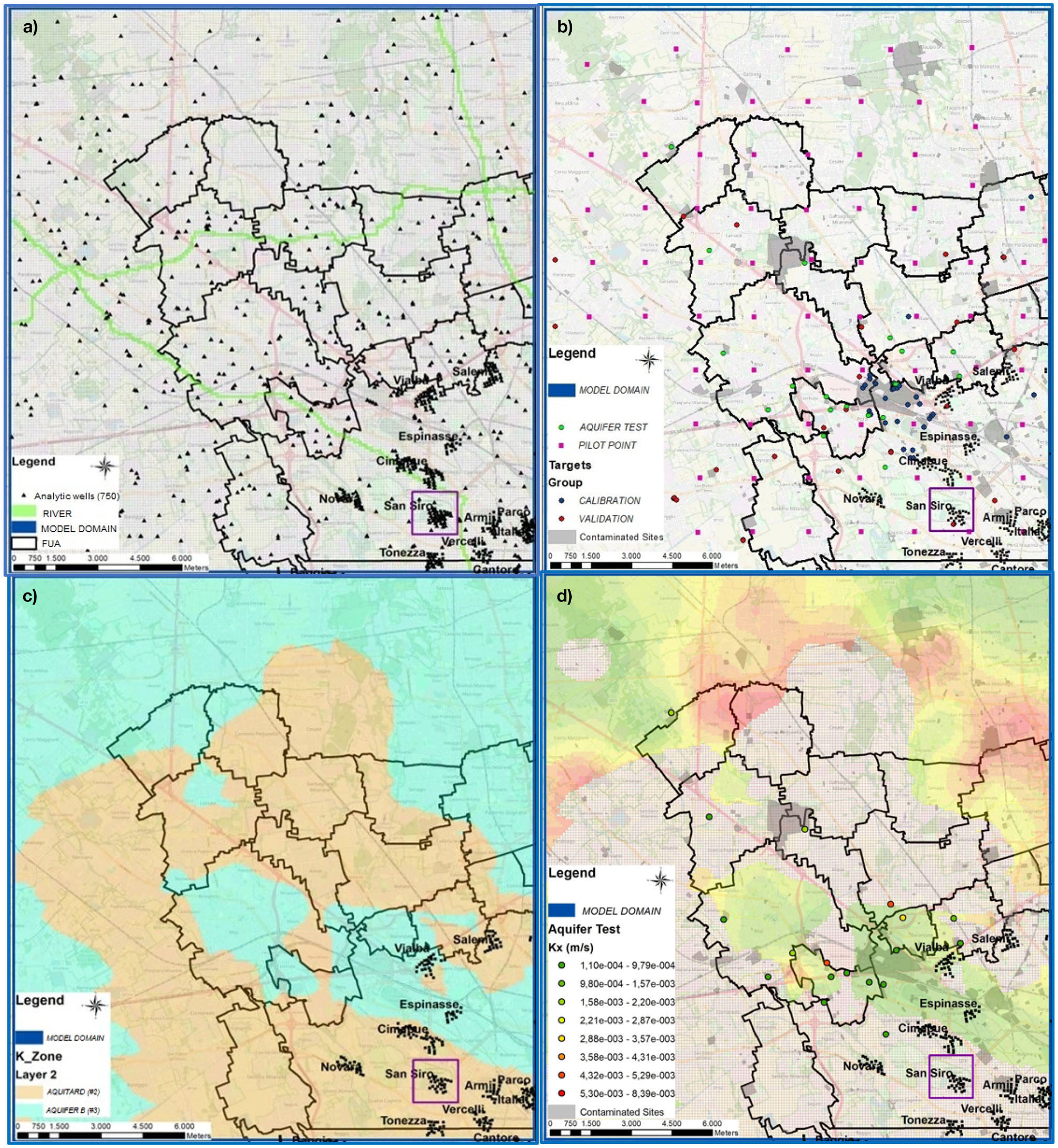
Groundwater model: (a) boundary conditions, grid, and internal condition; (b) Pilot Point (PP) positions and targets used for calibration (blue) and validation (red); (c) example of different zones used in calibration process for Layer 2 and (d) calibrated hydraulic conductivity distribution for Layer 2 in the deterministic process. The violet squared area is the San Siro pumping station, where the particles are located for the backtracking analysis.
The model has been calibrated in a steady state, as described in Colombo et al. (2019), using head values from 63 piezometers using the inverse parameter estimation code PEST (Doherty, 2010). The spatial variations in hydraulic conductivity are estimated by using a pilot point (PP) approach for each of the hydrogeology units (A and B). An anisotropy ratio between the horizontal direction (Kxx = Kyy) and the vertical direction (Kzz = 0.1Kxx) is applied. Four different zones, where the PPs are able to interpolate (using Kriging with an exponential variogram), the K-values have been set (zone 1 for Aquifer A, zone 3 for Aquifer B, zone 2–4 respectively for aquitard and lenses in Aquifer B). As suggested by Doherty (2015) and Moeck et al. (2020), using a high number of PPs, the variogram assumes less importance and only an estimation is required. During the process of inverse calibration, PEST is able to modify the PP values in order to minimize the objective target function (i.e., residual sum of squares expressed in m2, , where hobs is the observed head and hsim is the computed head) in subsequent iterations. Expert knowledge in this framework has been used to assign input values to the PPs representing aquifer tests performed in the study area (i.e., characterization of contamination site and new hydraulic barrier installations). For these PPs, as the hydraulic conductivity values have been estimated by a test (i.e., pumping tests), the boundary range is narrower compared to the others (+/- 0.5 times the magnitude of the value) in order to constrain the PEST estimation in a “real geological” interval. PPs are distributed differently in each zone (83 in zone 1, 46 in zone 2, 117 in zone 3, and 71 in zone 4). The density of the PPs is proportional to the head observation number, as suggested by Christensen and Doherty (2008), and they are uniformly distributed within the domain except for the aquifer test points. In general, the PP density has to take into account the possibility of exploring the heterogeneity, which is needed to have a good fit with observations; on the other hand, the more PPs are considered, the more complex is the inverse parameter estimation with its higher computational time. After this step, a singular value decomposition (SVD), in conjunction with a Tikhonov regularization, is applied in order to have a stable inverse process and to consider prior information (which includes the expert knowledge) into the model to obtain a reasonable geological structure. The subsequent step is to combine PPs with a NSMC analysis (Tonkin and Doherty, 2009) to provide spatial variations in the K-field. A total of 400 different parameter sets are generated through a random log-normal distribution based on the provided upper and lower parameter range (Table 1).
Table 1
| Geological zone | Initial level | Lower limit | Upper limit |
|---|---|---|---|
| 1 | 10−4 | 10−5 | 10−2 |
| 2 | 10−6 | 10−8 | 10−6 |
| 3 | 10−5 | 10−5 | 5 × 10⁻³ |
| 4 | 10−6 | 10−8 | 10−6 |
Hydraulic conductivity in m/s (initial and bounding values) of the parameter used under NSMC (for the geological zones description see Supplementary Figure 1).
The parameter sets are modified in the null-space projections and are adapted from the base model. In other words, PEST decomposes the parameter space into two perpendicular sub-spaces (solution and null-space). The first space is the representation of parameter combinations that can be estimated on the current field used for the calibration. The parts not “explained” in the solution space are spanned into the null-space (i.e., the second space). Each generated random parameter is therefore projected into the calibration null-space and the solution-space component is removed, as it is replaced with the calibrated parameter field from the base model. As the groundwater model is not linear, the stochastic parameter field needs to be re-calibrated. One option is a two-iteration method calibration. The final objective target function is then compared to the desired objective function to keep only the best calibrated K-distributions. Alberti et al. (2018) considered an arbitrary threshold value of the objective function corresponding to the objective function values of the initial deterministic calibrated model, while Moeck et al. (2020) considered both the expected measurement error and structural model error (to avoid overfitting).
In this analysis, following Alberti et al. (2018), the threshold has been set to 35 m2, corresponding to the objective function value of the “native” (primary) calibrated model. From the total set of 400 random models, 64 were discarded and 336 accepted for the further analyses (as presented in Supplementary Figure 3). Generally, the results in terms of probability in the study area are not different (in Supplementary Figure 4 shows the differences, while in Supplementary Figure 5 is shown the particle frequency distribution in Layer 2). The scheme of the adopted methodology is represented in Figure 3.
Figure 3
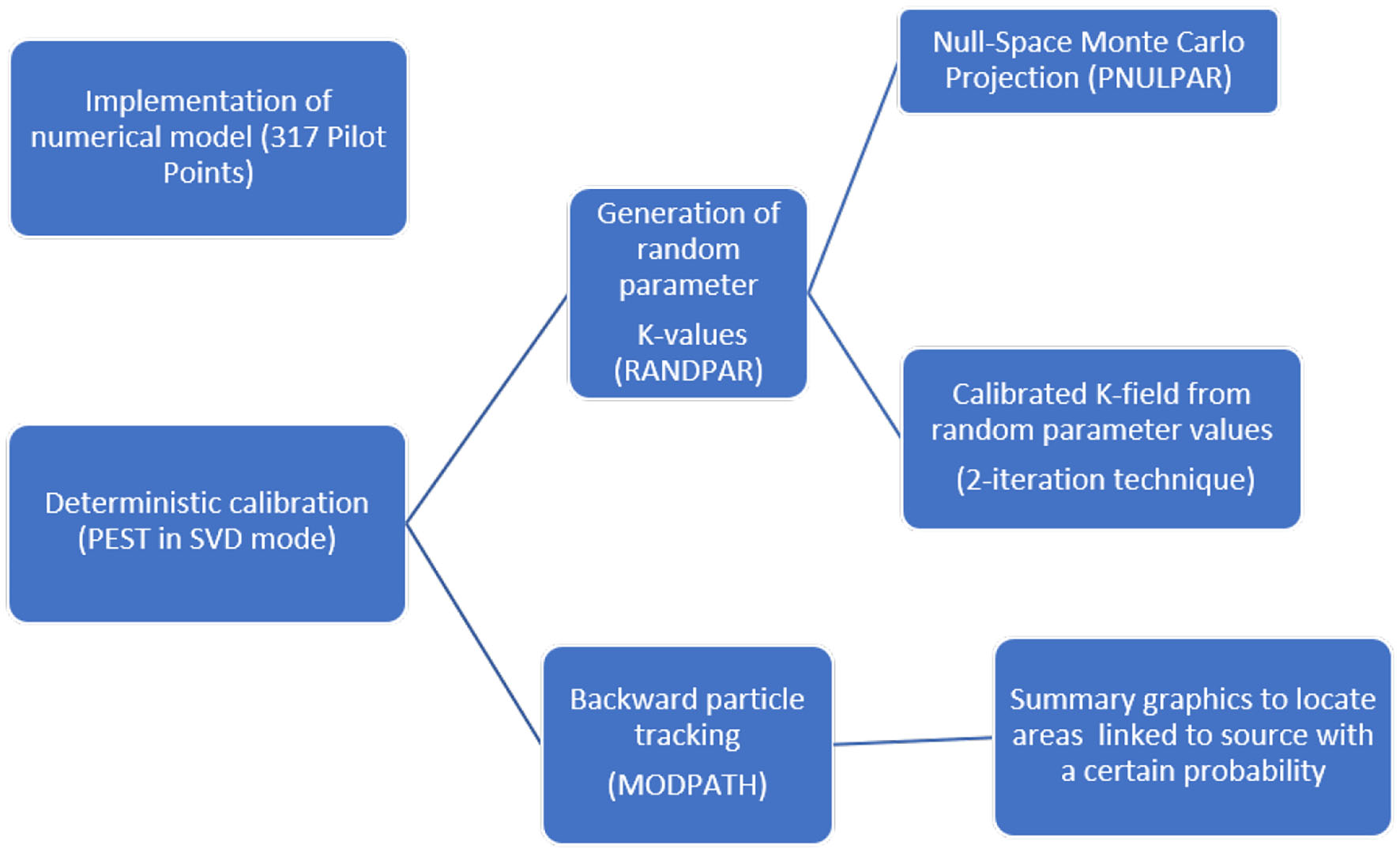
Conceptual flowchart for the PT+NSMC methodology.
In the literature, several examples of the NSMC method with different uses have been presented: from calibration purposes (Tonkin and Doherty, 2009; Doherty, 2015) to diffuse pollution assessment (Alberti et al., 2018) and from assessing aquifer pathways (Moeck et al., 2020) to testing barrier effectiveness (Formentin et al., 2019).
2.3. Integration of Particle Tracking and NSMC
To assess the most likely source area of the PCE contamination in the San Siro pumping wells in Milano and to identify the most likely occurring flow path, the particle backtracking technique has been applied by using the code MODPATH v.5 (Pollock, 1994). For all accepted hydraulic conductivity fields, 3D backward particle tracking has been carried out from most contaminated pumping well (well N°500), where the detected concentrations of PCE are historically higher than the threshold limit for drinking water set by the Environmental Ministry of Italy (2001). Figure 4 provides details about the area of the San Siro pumping station. In general, the wells of the Milano pumping stations are screened in Aquifer B, which is mostly protected by a clay lenses of variable thickness (between 1 and 3 m) whose extension is shown in Figure 2d. Figure 4 shows the cross-sections obtained from the pumping station well log-stratigraphy, where pumping well N°500 is screened in three different layers. The particles have been computed based on a “screen-position” hypothesis: since wells can screen more than one layer and so the actual depth of the contamination is uncertain, it has been assumed that the number of particles can be distributed in different modeled layers. Then, for well N°500, a total of three particles are positioned basing on the screened levels in permeable layers (Layer 5,7, and 9), as the contaminant is considered diluted along the screened length of the well.
Figure 4
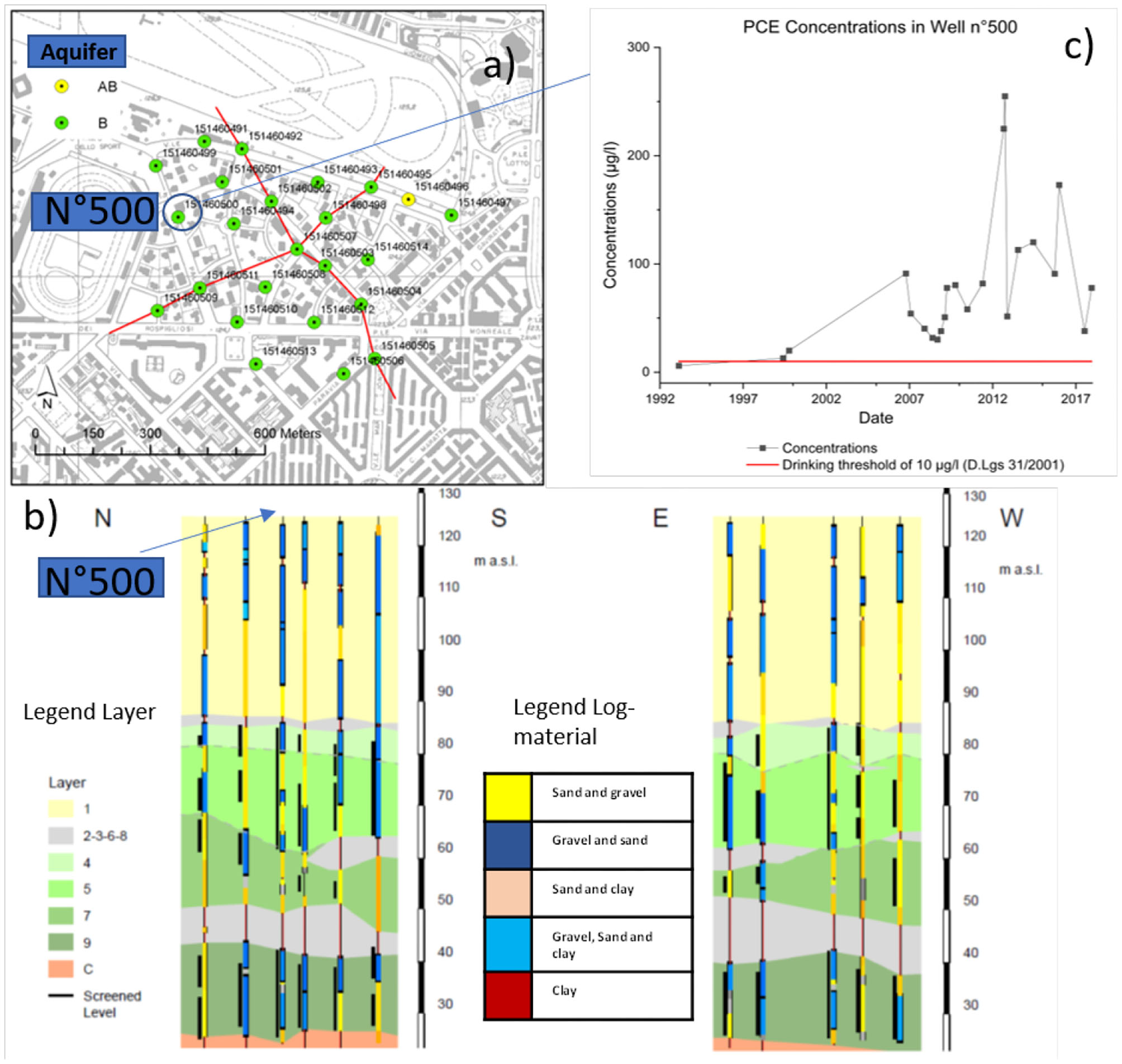
Technical layout of the San Siro pumping station: (a) position of the San Siro pumping wells, (b) cross-sections reporting stratigraphic well logs (the colors along each well represent the different materials); the color in the cross-section represents the different layers and (c) the PCE concentrations for the period 1992–2017 in well N°500 where the particles were placed.
3. Results and Discussion
Figure 5 shows the values of the objective function before and after the K-field re-calibration (paragraph 2.2). It can be seen that the randomly generated K-fields are generally “not calibrated” as generated by a “classical” Monte Carlo process: they have higher objective functions than the posterior calibration (399 models are not calibrated compared to the objective function of the “native” deterministic model during the first random extraction).
Figure 5
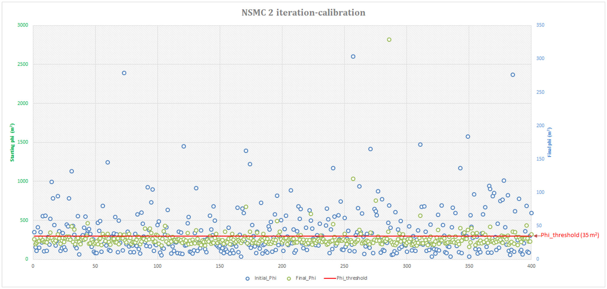
Comparison between the initial objective function (RANDPAR) and the final objective function obtained with the two-iteration process (SVD). The red line represents the threshold objective function limit (35 m2) used to retain the models with a good misfit to track particles.
3.1. Spatial Distribution of K-field Realization
During the calibration process, the hydraulic conductivity (K) random distributions are estimated over the available prior knowledge of the geological setting. Figure 6 shows the variability of the K pattern in some of the randomly generated realizations. The areas where the K-values are higher generally remain the same spatially. For example, in the northern part of the model, the extension of the high permeability zone (in white) changes the shape but remains located in the upper part of the area. This area is affected by limited information (only a few targets are available), and for this reason the uncertainty has a strong influence on the realizations. On the other hand, in the central area of the model (near the San Siro pumping station), the density of information (target measurements) is higher and the realizations are less influenced by the lack of observations. At these locations, the information contained in the head measurements is able to constrain the parameter estimation process.
Figure 6
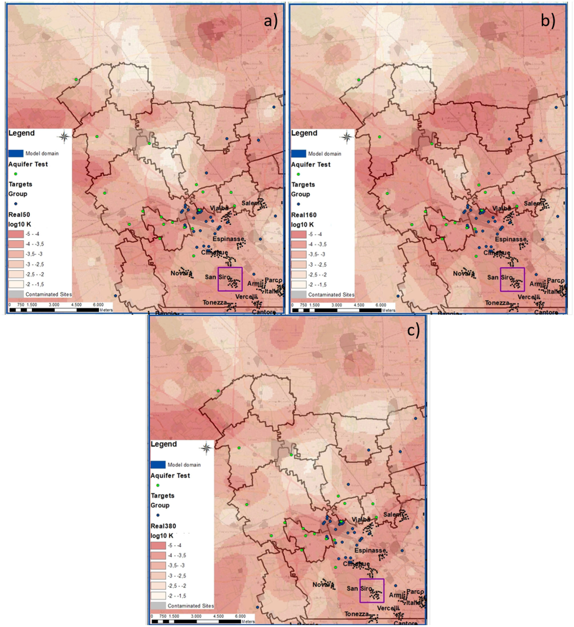
K distribution for Aquifer A for three randomly selected parameter realizations (a–c). The K values are shown as log10 values, where white and red areas show higher and lower K, respectively. Blue dots represent the head targets and green dots represent the aquifer tests.
3.2. Mapping the Backward NSMC Particle Tracking: the Probability Associated With the Source Areas of Contamination
Similar to Alberti et al. (2018) and Moeck et al. (2020), a computation of the number of particles crossing the model cells has been carried out, considering all different accepted simulations. Figure 7a represents the particle frequency distribution for all calibrated K-fields and for all model layers. For areas delineated with high pathline density (i.e., higher particle passage frequency), it is possible to delineate the most likely area that can contain one or more PS and it allows to apply the criterion “more probable than not.” It is important to remember that, also in those areas where the frequency is low, the possibility to find a source area is still not negligible. Most of the water pumped from the well is collected from a central narrow line whose frequency is higher than 10%. Superimposing the AGISCO database (from ARPA Lombardia, 2019) with these results (Figure 7), it is possible to underline the contaminated sites that are more probable to be responsible for the contamination detected in well N°500. The single pathline is comparable to the path with the highest pathline density. In this case, a single pathline can therefore be used as an initial screening tool.
Figure 7
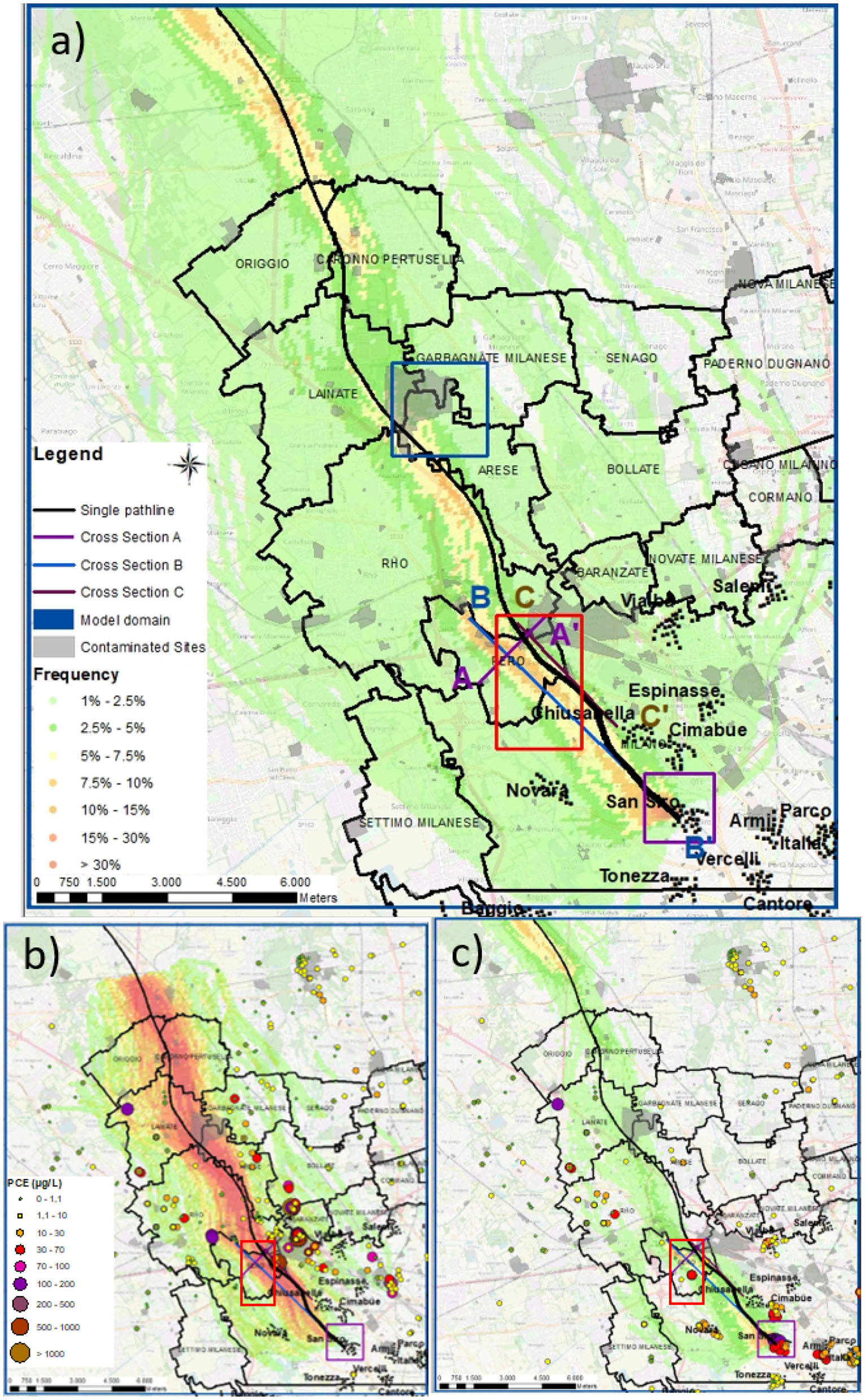
Particle frequency distribution of the ensemble backtracked pathlines for (a) all layers, (b) Aquifer A, and (c) Layer 5, representing the more affected sector of Aquifer B. Particle tracking has been carried out for all 336 accepted and re-calibrated model realizations. To represent the particle passage frequency, a threshold value of 1% was set in all maps. Black lines represent the pathlines resulting from the native deterministic model.
Figure 7a shows that there are few contaminated sites (Provincia di Milano, 1992, 1994) falling in the area having a higher probability (in yellow), whereas the majority of them fall in green areas having a low probability. Considering a probability higher than 10%, two industrial districts (represented in red and blue) can be considered the most probable source of the San Siro PCE contamination. Nevertheless, even if the backtracking PT assigns the same probability to those districts, the distance from well N°500 has to be considered. Indeed, chlorinated hydrocarbon plumes can be very long as natural attenuation needs anoxic aquifer conditions. However, the further the contaminated target is from the potential source, the less probable for that source to be responsible (McGuire et al., 2004). For this reason, as the red rectangle is closer to well N°500 in the San Siro pumping wells (approximately 6 km) compared to the blue rectangle (approximately 12 km), it can be stated that the latter has a globally lower probability of being responsible.
In order to better identify the contaminated sites and to clarify the contamination paths, two different maps have been prepared separating the two aquifers: Figure 7b shows the probability based only on particles flowing in Aquifer A, whereas Figure 7c represents the probability only in Layer 5, which can be considered representative of Aquifer B because most of the particles flow within this hydrogeological unit.
The following analysis of the particle paths in each aquifer was applied in order to narrow the areas directly impacted by the contamination:
In Aquifer A, the area with higher frequency (more than 15%) is more evident, which was used to restrict the analyses and then to find the potential responsible site.
In Aquifer B, the probability is significantly less than 10%. This map has the advantage to show that the withdrawals of the Novara pumping station are high enough to affect the flow direction in Aquifer B, acting as a “hydraulic barrier”, protecting the San Siro pumping station.
3.3. Analyses of the Cross-Sections and Discussion
In order to understand how the contamination can move and reach the screens of well N°500, it is also useful to analyze, through some cross-sections, the probability distribution of particles in the vertical direction. The represented particle frequencies have been computed summing the number of passages for each cell (the model coordinates are row and column) and dividing it by the total sum in each column (Figure 8): for example, in the cell coordinate (155;116), 29% of total particles crossing this specific column (whose total is indicated with ∑ in Figure 8) pass in Layer 1, whereas 2% pass in Layer 2, representing the shallow aquifer A and the aquitard, respectively. To present the advantages of this analysis, two different cross-sections (Figure 7a) have been drawn near the red squared area. To complete the analysis, a third cross-section is presented in the Supplementary Material (Supplementary Figure 7).
Figure 8
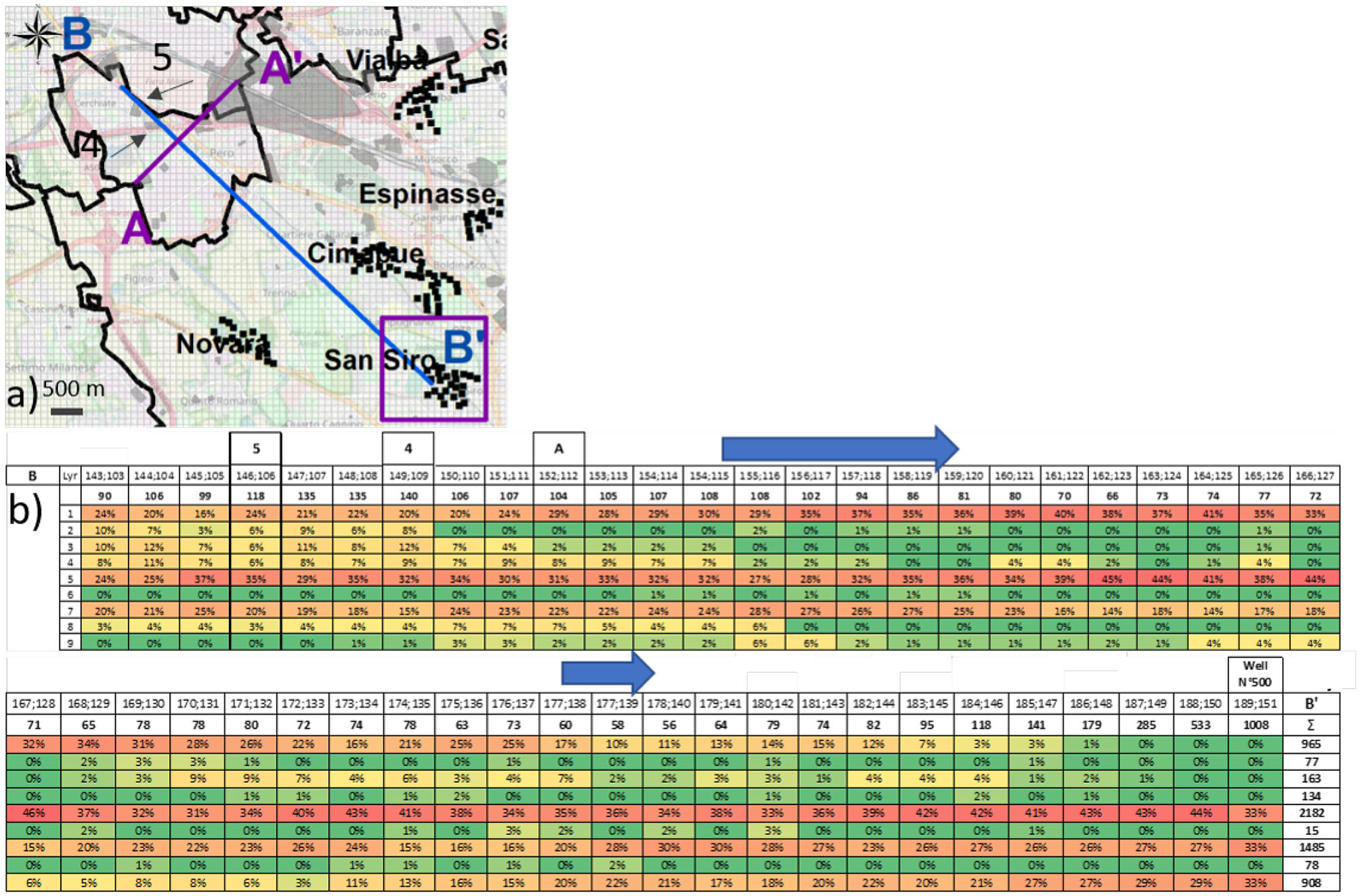
(a) Cross-section B, oriented NW-SE (BB') with the blue arrow indicating the flow direction: line one shows the cell coordinates, line two shows the sum of particles passing in each vertical column and then the percentage for each layer, and the last column represents the number of particles for each layer; (b) zoom of Figure 7, showing the area and two different industrial sites (4 and 5). The hydrogeological cross-section is shown in the Supplementary Figure 6B.
Longitudinal cross-section B (Figure 8): this is oriented along the main flow direction (NW-SE) and stretches for 7 km, starting from the red square to the San Siro pumping station. This representation allows to show in detail the vertical migration of the contamination along the main flow direction. Starting from the screens of well N°500 (cell 189;151) and backtracking the particle pathlines from there, Figure 8 shows that the particles flow only in Aquifer B (Layer from 5 to 9), but they are suddenly (cell 182;144) able to partially reach the shallower layers. Continuing northward, the number of particles in Layer 9 and 7 progressively decreases (cell 166;127), and, simultaneously, they increase in the more permeable upper Layers 5 and 1; due to the presence of a high number of clay lenses, Layers 2–4 are not significantly interested by the particles. As soon as a clay layer becomes discontinuous or disappears (from cell 154;114), the particle frequencies also increase in those layers, and similar percentages are consequently present in Layers 1 to 5, corresponding to industrial sites 4 and 5. These results show that contamination released in Aquifer A, 7 km from San Siro, is able to reach the upper part of the screen at well N°500 (corresponding to Layer 5). In contrast, in order to contaminate the deeper screens (Layer 7 and 9), PCE would have to be mainly released directly in the deeper part of Aquifer B, as few particles are able to cross the clay strata underneath Layer 5.
Transverse cross-section A (Figure 9): this is orthogonal to the main flow direction and stretches for 1.5 km. The capital letter B indicates the crossing point with the longitudinal cross-section. Figure 9 shows that at the red squared area, a large part of particles traverse Layer 1 and 5 where the particle sum is 239 and 212 respectively. Nevertheless, some differences can be noticed moving to the right and left of the B crossing point. On the right side, moving toward the industrial site 2, frequencies are quite similar from Layer 1 to 5 as displayed by the cross-section B in the cell (149;109). On the left side, toward the industrial site 3, frequencies are decreasing in Layer 2–4, indicating that here clay lenses are able to better separate Aquifer A from Aquifer B. Summarizing the results, it is possible to affirm that a PCE release in the shallow aquifer at site 2, 4, and 5, compared to sites 1 and 3, has a higher probability to be responsible for the contamination detected in well N°500 (mainly for screens positioned in Layer 5, as shown in Figure 8). On the other hand, for the contamination detected in screens located in Layers 7 and 9, a direct release (i.e., dry well) in the deeper part of Aquifer B should be hypothesized. Results show how the stochastic approach, combined with backtracking PT, is able to display the probability of the advective pathways followed by the contaminant.
Figure 9
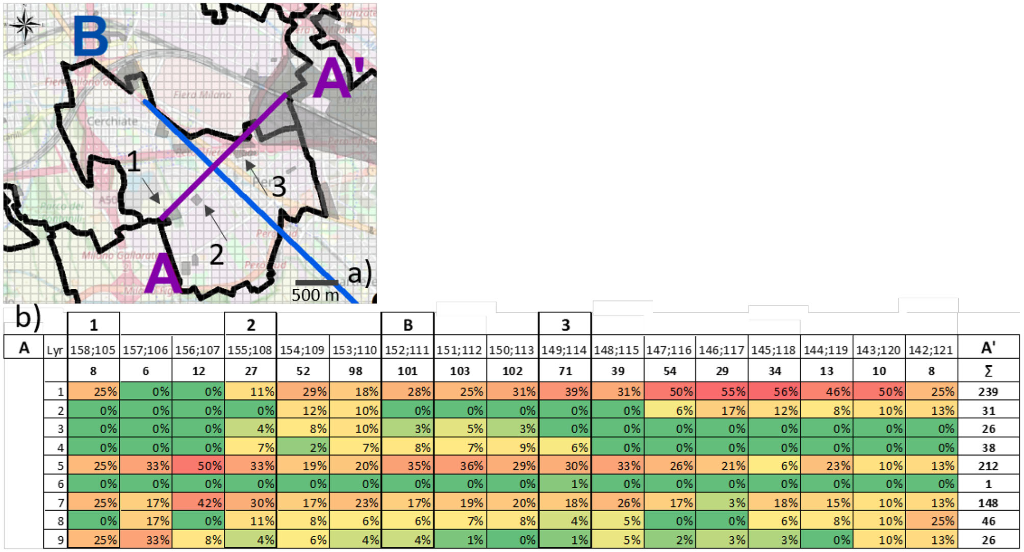
(a) Cross-section A, oriented SW-NE (AA′): line one shows the cell coordinate, line two the sum of particles passing in each vertical column and then the frequency for each layer, and the last column the count of particles for each layer; (b) zoom of Figure 7, showing the area and three different industrial sites (1, 2, and 3). The hydrogeological cross-section is shown in the Supplementary Figure 6A.
Stochastic particle tracking (PT+NSMC) is an innovative tool that can be helpful in the search for contamination source areas and plume monitoring. Its simplicity and versatility allows several advantages such as the ability to perform multiple analyses based on the same results, indeed two possible outcomes have been presented: (1) plan map (x,y) of the particle passage frequency in each cell of the model domain, showing all the possible pathlines that the contaminant can follow starting from a specific location, reached by the contamination, considering the uncertainty related to the hydraulic conductivity. The main advantage of the maps is that they allow us to consider a global frequency (i.e., counts all the particles belonging to a specific layer or group of layers) in order to locate the more likely area to be investigated by the installation of new piezometers or the characterization of brownfield areas. On the contrary, these maps are not able to link the vertical passage of the contamination (i.e., it would be necessary to produce as many maps as the number of layers); (2) vertical cross-sections representing the distribution of the particles cell by cell as a function of the layer (z), able to represent the impact of the contamination in each model layer and to give a 3D vision if orthogonal cross-sections are used. The advantage of these analyses is the calculation of the number of particles per vertical column and therefore the frequency for each layer (i.e., accounting for the particles passing through a specific cell) in order to show the contamination impact relative to a single cell. However, the vertical cross-section is representative of a specific area and as many different cross-sections as the number of different contaminated sites should be made (i.e., a reconstruction in a greater detail of the contamination paths). The two analyses are complimentary and can be used together to identify both potential contamination sources (i.e., higher frequency in the plan map) in order to find appropriate areas to install monitoring wells and suitable positions for the well screens (i.e., in the more contaminated layer computed in the vertical cross-section). However, this methodology shows some limitations that can be further improved. For example, a preliminary linear uncertainty analysis (Moore and Doherty, 2005; James et al., 2009; Dausman et al., 2010; Moeck et al., 2015, 2020) can be carried out in order to identify the most important parameters linked to the uncertainty and likely to be used in the NSMC procedure: for example, porosity, well abstractions, the vertical recharge, and the boundary conditions can be considered in the analyses. In this paper, only the hydraulic conductivity has been considered as uncertain because concerning the porosity, previous analyses showed that the model is not sensitive to this parameter (Colombo et al., 2019); well abstraction data have been provided by water managers so are considered to be only slightly uncertain. To deal with BC's, the choice has been to use a large model domain in order to set them far away from the area of interest and therefore would have a low influence. Since the results obtained by the deterministic pathline and the higher pathline density area obtained with NSMC are coherent (Figure 7), it is possible that the flow path is mainly controlled by the BCs and therefore the subsurface heterogeneity might be less important. For this reason, the influence of the BCs it will be further investigated in the future. In addition, as reported by Chow et al. (2016), particle tracking provides an approximation of groundwater flow paths and results can differ between simulators because of velocity approximations which are used for computation of the particle tracks. In the model presented here, a regular grid has been used due to the domain dimensions, and the choice was to apply the option “pass through weak sinks” in order to not terminate any particle and as a factor of safety from an environmental point of view. Thanks to the unstructured grid of the MODFLOW-USG version (Panday et al., 2013), it also would be possible to reduce the particle tracking numerical error using a refined grid where wells fall in the area of interest. Another possible improvement of the proposed methodology could consider the combination of stochastic results with contaminant concentrations detected in the monitoring network. Overlapping this information would exclude some areas removing the pathlines passing through clean wells, following the methodology presented in Formentin et al. (2019). Finally, in dense urban contexts, the results are not able to guarantee a unique liable area for the contamination (i.e., the presence of many contaminated sites along the main water flow direction as in cross-section B). Therefore, it can be coupled with other analyses to further reduce the list of potential responsible sites. For example, some statistics about the general behavior of chlorinated solvent plumes can be considered, like those presented in McGuire et al. (2004). Considering a sample of 45 chlorinated solvent sites (managed through monitored natural attenuation), 96% of the plumes were shorter than approximately 1.5 km and over a sample of 25 sites 68% of the remediation time-frame was less than 30 years. According to these statistics, a more distant potential source (e.g., the blue squared area in Figure 7) is less likely to be responsible and therefore the spatial range likely to contain the contamination source can be limited, weighting the probability on the target distance or the contaminant travel time. These ideas could be a future improvement of the proposed methodology.
4. Conclusions
The northwestern area in the Milano Functional Urban Area is affected by a strong presence of chlorinated hydrocarbons, originating from several contaminated sites historically present in the territory. Over the last years, this contamination has posed important safety problems in the intake area of the water supply wells of Milano. For this reason, the remediation of groundwater for drinking water purposes has become a major problem for water managers; on one hand, the water treatment procedures became more onerous both in terms of management and new plants (like new active carbon filter installations), but, on the other hand, the cost of the raw water clean-up has to be imposed on the citizens within the water bill costs. In this situation, the Polluter Pay Principle becomes crucial: its application to groundwater contamination due to the “more probable than not” responsible source is able to help charge the cost of site remediation and (mainly) the treatment costs of the water extracted for public use. The support of a groundwater model is very useful to study the contamination pathways, but, especially in the presence of multiple possible sources, the deterministic simulation fails as the uncertainties strongly influence the results both in terms of groundwater flow and in terms of contaminant transport. In this context, new methodologies and models have been developed (Alberti et al., 2018; Moeck et al., 2020). One innovative methodology is to combine particle backtracking with a constrained Monte Carlo approach (i.e., considering the uncertainties linked to the hydraulic conductivity). This combination has been developed throughout this paper to identify PCE point sources in urban areas. Starting from one of the pumping wells most contaminated by PCE in the San Siro pumping station, a particle backtracking stochastic analysis has been developed. Considering all the accepted K-field realizations (336), all the contaminated sites within the non-zero probability areas must be considered as potential sources for this pollution. However, in such a densely industrialized zone, this result is not able to narrow the area where the actual source of the contamination can be identified. Then, a further analysis has been developed in order to: (1) narrow the suspected areas considering the higher particle density, recognizing as possible sources only five sites among several others present upstream of the detected contamination; (2) study the particle paths in greater detail dividing the map results into two different hydrogeological units (Aquifer A and Aquifer B) using a high vertical discretization of the model (nine layers); and (3) provide vertical cross-sections of the particle passage frequency for selected suspected areas. In conclusion, particle tracking with Monte Carlo can be used as a method to identify the “more probable than not” areas potentially responsible for contamination detected in sensitive targets. For this reason, the method can be very helpful to the public authorities as a decision support tool to prepare a ranking list of possible potential responsible sites for contamination and to design a suitable well monitoring network. In densely industrialized districts, the proposed procedure is not able to identify just one source site with certainty and it needs to be coupled together with other analyses to provide strong evidence of liability. This method provides a new basis for future modelers, where the geological uncertainty plays a fundamental role for a reasonable and responsible assessment of the polluters.
Statements
Data availability statement
The data analyzed in this study is subject to the following licenses/restrictions: Data about contaminated sites are confidential due to ongoing legal procedures. Requests to access these datasets should be directed to Regione Lombardia through the online form ambiente_clima@pec.regione.lombardia.it.
Author contributions
LC, PM, and LA developed the model and carried out the analyses. LC and PM contributed to the development of Excel Macros and scripts that enabled the automated analysis of counting particles herein. LC, PM, and LA also contributed to the higher-level workflow. LA provided expert knowledge for defining the conceptual model. LC, PM, and MA wrote the initial draft. However, all authors contributed to the writing of the manuscript.
Funding
The authors would like to acknowledge funding from the Interreg Central Europe Project (CE No. 32 AMIIGA - Integrated Approach to Management of Groundwater Quality in Functional Urban Areas).
Acknowledgments
The authors would like to acknowledge Regione Lombardia for the data availability on the contaminated sites (information and shapefile-AGISCO DB) and contaminant concentration data (i.e., PCE concentration). We would also like to acknowledge Eng. Giovanni Formentin and John Doherty for supporting the methodology and scripts. We thank the Milano public water manager (Metropolitana Milanese S.p.A.) for the information and data about the Milano aqueduct wells. Finally, we would like to acknowledge the reviewers that help us to improve the text and the quality of the manuscript.
Conflict of interest
The authors declare that the research was conducted in the absence of any commercial or financial relationships that could be construed as a potential conflict of interest.
Supplementary material
The Supplementary Material for this article can be found online at: https://www.frontiersin.org/articles/10.3389/fenvs.2020.00142/full#supplementary-material
References
1
Alberti L. Azzellino A. Colombo L. Lombi S. (2016). Use of cluster analysis to identify tetrachloroethylene pollution hotspots for the transport numerical model implementation in urban functional area of milan, italy. Int. Multidiscipl. Sci. GeoConfer. Surv. Geol. Min. Ecol. Manage.1, 723–729. 10.5593/SGEM2016/B11/S02.091
2
Alberti L. Brogioli G. Formentin G. Marangoni T. Masetti M. (2007). Experimental studies and numerical modeling of surface water-groundwater interaction in a semi-disconnected system, in IAH Congress, Groundwater and Ecosystems (Lisbon).
3
Alberti L. Colombo L. Formentin G. (2018). Null-space monte carlo particle tracking to assess groundwater pce (tetrachloroethene) diffuse pollution in North-Eastern Milan functional urban area. Sci. Total Environ.621, 326–339. 10.1016/j.scitotenv.2017.11.253
4
Alberti L. Lombi S. Zanini A. (2011). Identification de sources d'hydrocarbures aliphatiques chlorés dans une zone résidentielle en italie par la méthode d'essai de pompage intégral. Hydrogeol. J.1:76. 10.1007/s10040-011-0742-1
5
Alberti L. Marchesi M. Trefiletti P. Aravena R. (2017). Compound-specific isotope analysis (csia) application for source apportionment and natural attenuation assessment of chlorinated benzenes. Water9:872. 10.3390/w9110872
6
Alderuccio M. Cantarella L. Ostoich M. Ciuffi P. Gattolin M. Tomiato L. et al . (2019). Identification of the operator responsible for the remediation of a contaminated site. Environ. For.20, 339–358. 10.1080/15275922.2019.1657521
7
ARPA Lombardia (2019). Anagrafe e gestione integrata dei siti contaminati (agisco).
8
Barilari A. Quiroz Londoño M. Paris M. Lima M. Massone H. (2020). Groundwater contamination from point sources. a hazard index to protect water supply wells in intermediate cities. Groundwater Sustain. Dev.10:100363. 10.1016/j.gsd.2020.100363
9
Bauer S. Bayer-Raich M. Holder T. Kolesar C. Müller D. Ptak T. (2004). Quantification of groundwater contamination in an urban area using integral pumping tests. J. Contamin. Hydrol.75, 183–213. 10.1016/j.jconhyd.2004.06.002
10
Beretta G. P. Avanzini M. Pagotto A. (2004). Managing groundwater rise: experimental results and modelling of water pumping from a quarry lake in milan urban area (italy). Environ. Geol.45, 600–608. 10.1007/s00254-003-0918-7
11
Beretta G. P. Civita M. Francani V. (1992). Idrogeologia per il disinquinamento delle acque sotterranee: tecniche per lo studio e la progettazione degli interventi di prevenzione, controllo, bonifica e recupero. Milano: Pitagora Editrice Bologna.
12
Bini A. (1987). L'apparato glaciale wurmiano di Como (Ph.D. thesis) Tesi di Dottorato di Ricerca, Università di Milano, Milan, Italy.
13
Carrera J. Alcolea A. Medina A. Hidalgo J. Slooten L. J. (2005). Inverse problem in hydrogeology. Hydrogeol. J.13, 206–222. 10.1007/s10040-004-0404-7
14
Cavallin A. Francani V. Mazzarella S. (1983). Studio idrogeologico della pianura compresa fra adda e ticino. Milano: Costruzioni.
15
Chamizo-González J. Cano-Montero E. I. Muñoz-Colomina C. I. (2018). Does funding of waste services follow the polluter pays principle? The case of Spain. J. Clean. Prod. 183, 1054–1063. 10.1016/j.jclepro.2018.02.225
16
Chow R. Frind M. E. Frind E. O. Jones J. P. Sousa M. R. Rudolph D. L. et al . (2016). Delineating baseflow contribution areas for streams–a model and methods comparison. J. Contamin. Hydrol.195, 11–22. 10.1016/j.jconhyd.2016.11.001
17
Christensen S. Doherty J. (2008). Predictive error dependencies when using pilot points and singular value decomposition in groundwater model calibration. Adv. Water Resour.31, 674–700. 10.1016/j.advwatres.2008.01.003
18
Colombo L. Alberti L. Mazzon P. Formentin G. (2019). Transient flow and transport modelling of an historical chc source in north-west milano. Water11:1745. 10.3390/w11091745
19
Covucci D. (2019). The “polluter pays principle”: environmental liabilities and scientific evidence under the italian law system. Acque Sotterranee Ital. J. Groundwater8, 69–72. 10.7343/as-2019-427
20
Dausman A. M. Doherty J. Langevin C. D. Sukop M. C. (2010). Quantifying data worth toward reducing predictive uncertainty. Groundwater48, 729–740. 10.1111/j.1745-6584.2010.00679.x
21
De Sadeleer N. (2014). Polluter Pays Principle. Oxford: OUP.
22
Directive 2004/35/EC (2004). Member States Have Until the End of April 2007 to Transpose This Directive Into Domestic Law.
23
Doherty J. (2010). Methodologies and software for pest-based model predictive uncertainty analysis. Watermark Numer. Comput. 1–33.
24
Doherty J. (2015). Calibration and uncertainty analysis for complex environmental models. Watermark Numer. Comput. 1–224.
25
Environmental Ministry of Italy (2001). Legislative Decree no. 31, Approving the Directive 98/83/ce Based on the Drinkable Water. Gazzetta Ufficiale.
26
Environmental Ministry of Italy (2006). Legislative Decree no. 152 Approving the Code on the Environment.
27
Formentin G. Terrenghi J. Vitiello M. Francioli A. (2019). Evaluation of the performance of a hydraulic barrier by the null space monte carlo method. Acque Sotterranee Ital. J. Groundwater. 8, 55–61. 10.7343/as-2019-420
28
Frind E. O. Molson J. W. (2018). Issues and options in the delineation of well capture zones under uncertainty. Groundwater56, 366–376. 10.1111/gwat.12644
29
Giovanardi A. (1979). Pollution by organic chloride compounds of the aquifers of the region of milan [contaminazione da composti organoclorurati delle falde idriche del territorio milanese]. Riv. Ital. d'Igiene39, 323–344.
30
Harbaugh A. W. (2005). MODFLOW-2005, the US Geological Survey Modular Ground-Water Model: The Ground-Water Flow Process. Reston, VA: US Department of the Interior; US Geological Survey.
31
Hunkeler D. Meckenstock R. U. Lollar B. S. Schmidt T. C. Wilson J. T. (2008). A Guide for Assessing Biodegradation and Source Identification of Organic Ground Water Contaminants Using Compound Specific Isotope Analysis (CSIA). Ada, OK: USEPA Publication.
32
James S. C. Doherty J. E. Eddebbarh A.-A. (2009). Practical postcalibration uncertainty analysis: Yucca mountain, nevada. Groundwater47, 851–869. 10.1111/j.1745-6584.2009.00626.x
33
La Vigna F. Sbarbati C. Bonfà I. Martelli S. Ticconi L. Aleotti L. et al . (2019). First survey on the occurrence of chlorinated solvents in groundwater of Eastern sector of rome. Rend Lincei Sci. Fisiche Nat.30, 297–306. 10.1007/s12210-019-00790-z
34
Luppi B. Parisi F. Rajagopalan S. (2012). The rise and fall of the polluter-pays principle in developing countries. Int. Rev. Law Econ. 32, 135–144. 10.1016/j.irle.2011.10.002
35
Masetti M. Poli S. Sterlacchini S. Beretta G. P. Facchi A. (2008). Spatial and statistical assessment of factors influencing nitrate contamination in groundwater. J. Environ. Manage.86, 272–281.
36
McGuire T. M. Newell C. J. Looney B. B. Vangelas K. M. Sink C. H. (2004). Historical analysis of monitored natural attenuation: a survey of 191 chlorinated solvent sites and 45 solvent plumes. Remediat. J.15, 99–112. 10.1002/rem.20036
37
Menichetti S. Doni A. (2017). Organohalogen diffuse contamination in firenze and prato groundwater bodies. investigative monitoring and definition of background values. Acque Sotterranee Ital. J. Groundwater6, 47–63. 10.7343/as-2017-260
38
Milon J. W. (2019). The polluter pays principle and everglades restoration. J. Environ. Stud. Sci. 9, 67–81. 10.1007/s13412-018-0529-y
39
Moeck C. Hunkeler D. Brunner P. (2015). Tutorials as a flexible alternative to guis: an example for advanced model calibration using pilot points. Environ. Model. Softw.66, 78–86. 10.1016/j.envsoft.2014.12.018
40
Moeck C. Molson J. Schirmer M. (2020). Pathline density distributions in a null-space monte carlo approach to assess groundwater pathways. Groundwater58, 189–207. 10.1111/gwat.12900
41
Moore C. Doherty J. (2005). Role of the calibration process in reducing model predictive error. Water Resour. Res.41:W05020. 10.1029/2004WR003501
42
Panday S. Langevin C. D. Niswonger R. G. Ibaraki M. Hughes J. D. (2013). Modflow–Usg Version 1: An Unstructured Grid Version of Modflow for Simulating Groundwater Flow and Tightly Coupled Processes Using a Control Volume Finite-Difference Formulation. Technical report, US Geological Survey.
43
Pollicino L. C. Masetti M. Stevenazzi S. Colombo L. Alberti L. (2019). Spatial statistical assessment of groundwater pce (tetrachloroethylene) diffuse contamination in urban areas. Water11:1211. 10.3390/w11061211
44
Pollock D. W. (1994). User's Guide for MODPATH/MODPATH-PLOT, Version 3: A Particle Tracking Post-processing Package for MODFLOW, the US: Geological Survey Finite-difference Ground-water Flow Model.
45
Provincia di Milano (1992). Indagini sulla presenza di composti organo-alogenati nelle acque di falda della Provincia di Milano. Technical report, Sistema Informativo Falda, Milano, Italy.
46
Provincia di Milano (1994). Acqua sotto i piedi. Technical report, Sistema Informativo Falda, Milano, Italy.
47
Regione Lombardia and ENI Divisione Agip (2002). Geologia degli acquiferi padani della regione lombardia.
48
Rojas R. Feyen L. Dassargues A. (2008). Conceptual model uncertainty in groundwater modeling: combining generalized likelihood uncertainty estimation and bayesian model averaging. Water Resour. Res.44:W12418. 10.1029/2008WR006908
49
Rumbaugh J. Rumbaugh D. (2011). Guide to Using Groundwater Vistas, Version 6. New York, NY: Environmental Simulations.
50
Schwartz P. (2018). The polluter-pays principle, in Elgar Encyclopedia of Environmental Law (Cheltenham, UK: Edward Elgar Publishing Limited), 260–271.
51
Segre M. (1987). Organic Chlorine Compounds Pollution of Milan Groundwater: Two Cases. Acqua Aria, 1.
52
Shouakar-Stash O. Frape S. Aravena R. Gargini A. Pasini M. Drimmie R. (2009). Analysis of compound-specific chlorine stable isotopes of vinyl chloride by continuous flow–isotope ratio mass spectrometry (fc–irms). Environ. For.10, 299–306. 10.1080/15275920903347628
53
Thornthwaite C. W. (1948). An approach toward a rational classification of climate. Geogr. Rev.38, 55–94. 10.2307/210739
54
Tonkin M. Doherty J. (2009). Calibration-constrained monte carlo analysis of highly parameterized models using subspace techniques. Water Resour. Res.45:W00B10. 10.1029/2007WR006678
55
Zahar A. (2018). Implementation of the polluter pays principle in China. Rev. Eur. Compar. Int. Environ. Law. 27, 293–305. 10.1111/reel.12242
Summary
Keywords
particle tracking, Null-Space Monte Carlo, Stochastic MODPATH, groundwater pollution, inverse modeling, uncertainty prediction, PEST
Citation
Colombo L, Alberti L, Mazzon P and Antelmi M (2020) Null-Space Monte Carlo Particle Backtracking to Identify Groundwater Tetrachloroethylene Sources. Front. Environ. Sci. 8:142. doi: 10.3389/fenvs.2020.00142
Received
24 April 2020
Accepted
27 July 2020
Published
25 September 2020
Volume
8 - 2020
Edited by
Teng Xu, Hohai University, China
Reviewed by
Ty Ferre, University of Arizona, United States; Christian Moeck, Swiss Federal Institute of Aquatic Science and Technology, Switzerland; John Molson, Laval University, Canada
Updates
Copyright
© 2020 Colombo, Alberti, Mazzon and Antelmi.
This is an open-access article distributed under the terms of the Creative Commons Attribution License (CC BY). The use, distribution or reproduction in other forums is permitted, provided the original author(s) and the copyright owner(s) are credited and that the original publication in this journal is cited, in accordance with accepted academic practice. No use, distribution or reproduction is permitted which does not comply with these terms.
*Correspondence: Loris Colombo loris.colombo@polimi.it
This article was submitted to Environmental Informatics and Remote Sensing, a section of the journal Frontiers in Environmental Science
Disclaimer
All claims expressed in this article are solely those of the authors and do not necessarily represent those of their affiliated organizations, or those of the publisher, the editors and the reviewers. Any product that may be evaluated in this article or claim that may be made by its manufacturer is not guaranteed or endorsed by the publisher.