Analysis and Classification of Stormwater and Wastewater Runoff From the Tijuana River Using Remote Sensing Imagery

Introduction

The coastal regions of Southern California are susceptible to coastal pollution from urban drainage. With respect to stormwater, a buildup of pollutants on land during the dry summer months are transported to coastal oceans during wet season events (Bay et al., 2003; DiGiacomo et al., 2004; Svejkovsky et al., 2010; Holt et al., 2017). Stormwater runoff from a large urban coastal environment contains sediments as well as bacteria, oil, fuel, and tire particles from automobiles, anthropogenic components from sewage, and fertilizer from agriculture (Reifel et al., 2009; Svejkovsky et al., 2010). This represents a hazard for the ecosystem and for public health in this coastal region, particularly during the rainy season (Ackerman and Weisberg, 2003). Often, during these events, bacteria levels of fecal indicator bacteria (FIB) and enterococcus (ENT) are as high as 15,000 CFU/100 mL in the ocean which can lead to significant health issues for beachgoers and surfers (Ackerman and Weisberg, 2003). EPA guidelines recommend FIB and ENT should not be greater than 100 CFU/100 mL¹. Recreational water activities should be avoided for at least 3 days after a rain event (Ackerman and Weisberg, 2003) since studies have shown an increase risk of gastrointestinal or other acute illness in surfers within that time period (Schiff et al., 2016; Arnold et al., 2017).

Analysis of stormwater runoff and wastewater plumes, for purposes of managing and minimizing health impacts to beach communities, with observational datasets are generally limited to in situ data collections and fixed stations. Remote sensing based assessments of plumes in Southern California have used various multispectral sensors with varying resolution including SeaWiFS optical radiometer (Nezlin and DiGiacomo, 2005), MODIS (1 km), Landsat-8 (15 to 30 m), and NOAA’s Advanced Very High-Resolution Radiometer (AVHRR) (1 km) (Nezlin et al., 2007; Warrick et al., 2007; Lahet and Stramski, 2010; Svejkovsky et al., 2010), all of which have significant limitations in terms of spatial, temporal and spectral resolution and cloud cover. In Holt et al. (2017), both SAR (5 to 150 m) and MODIS imagery were used to study stormwater runoff in the Southern California Bight. In Devlin et al. (2015), MODIS was also used to investigate the impact of stormwater plumes on coral reefs in the Great Barrier Reef.

Publicly operated wastewater treatment facilities in Southern California typically discharge treated wastewater offshore at depth, with the effluent largely mixing at depth and remaining below the thermocline. During limited occasions, maintenance requirements to a facility’s discharge system required the temporary diversion of treated wastewater closer to shore and at shallower depths. During such diversions, significant collections of both in situ and spaceborne remote sensing provided an opportunity to improve understanding of wastewater plume dynamics and impacts (Gierach et al., 2017; Trinh et al., 2017) as well as the biological response to increased nutrient levels (Reifel et al., 2009; Caron et al., 2017). The Tijuana River watershed is about 1,750 square miles of area that spans across the California – Mexico border (Figure 1). About 75 percent of the watershed is in Mexico, while the remainder is on the California side near Imperial Beach including the river mouth. Stormwater runoff plumes have been observed after rain events at the Tijuana River outlet. In addition, the frequent release of treated and untreated wastewater into the Tijuana River watershed has been documented to occur since the late 1990s. Both types of coastal plumes have been shown to impact the San Diego, CA, United States coastal region as well as the closely adjacent Mexico region, causing health concerns for beachgoers and residents. The two wastewater treatment plants of interest are the South Bay International Wastewater Treatment Plant (SBIWTP) located in San Diego, CA, United States and the San Antonio de los Buenos Wastewater Treatment Plant located in Tijuana, Mexico shown in Figure 1.

FIGURE 1

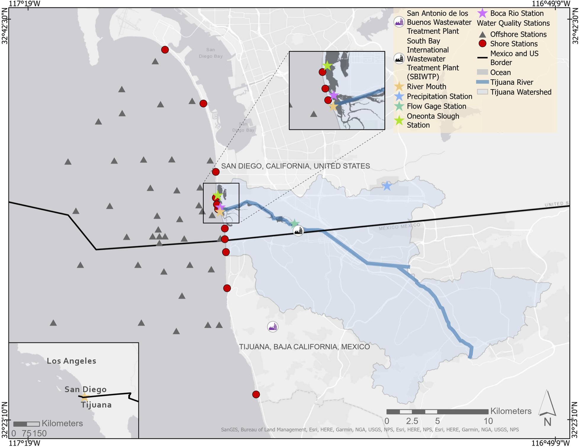
Figure 1. The Tijuana River Watershed. The water quality sampling stations from The City of San Diego Public Utilities are denoted by red points and gray triangles. Automatic water quality sampling stations from the NOAA National Estuarine Research Reserve System (NERRS) located in the estuary are symbolized as a purple (Boca Rio Station) and light green star (Oneonta Slough Station). The Tijuana River mouth is symbolized as a yellow star and the flow gauge station is a green star near the United States Mexico border. The precipitation station is the blue star located at the Brown Field Municipal Airport. The South Bay International Wastewater Treatment Plant (SBIWTP) is located in San Diego, CA near the United States Mexico border. The San Antonio de los Buenos Wastewater Treatment Plant is located in Tijuana, Mexico situated south of the watershed.

Stormwater runoff is largely tied to rain events, often carrying along multiple type of material and contaminants as mentioned earlier, and is monitored by a flow gauge station. The Tijuana River has raised particular attention due to the increasing occurrence of untreated wastewater released up river closer to the Tijuana population center that contains a high level of FIB effluent into the coastal area² as well as the reference of human fecal markers. The transport of both type of plumes is dependent on the nearshore circulation, with the San Diego coastal population notably greater than on the Mexico coastal side. For example, the San Diego Regional Water Quality Control Board reported wastewater pollution in the Tijuana River Watershed on February 6-23, 2017, where there was an incident of an estimated 28 million gallons (MG) of untreated wastewater released into the Tijuana River (see text footnote 2). This has caused major water quality and health issues particularly when transported northward into the large urban population in the San Diego area that live near the coast. In another recent case, during December 11–14, 2018, there was a wastewater spill of 7 million gallons per day, totaling an estimated 28 million gallons (see text footnote 2). More recently, from January 18–30, 2019, there were 610 million gallons that spilled in this region (see text footnote 1). In 2018, the San Diego Regional Water Quality Control Board sent a letter of intent to sue the United States Section of the International Boundary and Water Commission (USIBWC) for violations of the Clean Water Act and seeking improvements to the treatment of wastewater and reduction of accidental releases. Both the United States and Mexico are working toward a solution since the watershed is shared by both countries and continues to be an ongoing transboundary water issue.

The studies on stormwater and wastewater focused on the detection, extent, and impact of known separately occurring events and resultanting plumes but did not differentiate between plume types based on sensor responses. The only known studies on the detection and possible classification of wastewater in a coastal environment with remote sensing were in DiGiacomo et al., 2004; Marmorino et al., 2010; Seegers et al., 2017; Trinh et al., 2017; Gierach et al., 2017. In Gierach et al. (2017), Moderate Resolution Imaging Spectrometer (MODIS) and Satellite Aperture Radar (SAR) data were used to detect wastewater plumes during two diversion events in Southern California. The results showed that wastewater plumes could be identified by a decrease in sea surface temperature (SST) from MODIS and changes in the surface roughness from SAR. Another study by Trinh et al. (2017) utilized Landsat 8 Operational Land Imager (OLI) and MODIS imagery to derive SST and chlorophyll-a to investigate wastewater impacts and transport within Santa Monica Bay, California, after a third diversion event. We know of no published study using remote sensing that has successfully identified stormwater plumes from treated wastewater or raw wastewater plumes.

The goal of this study is to determine if the wastewater and stormwater plumes are optically distinct from each other, by examining differences in spectral reflectance and derived parameters, such as turbidity and colored dissolved organic matter (CDOM), in combination with in situ data, such as precipitation, enterococcus (ENT), and flow discharge rate. We hypothesize that these two plume types will have distinct spectral properties because stormwater plumes are likely to be dominated by sediments (Corcoran et al., 2010) and that wastewater is likely to be dominated by organic matter (DiGiacomo et al., 2004; Nezlin et al., 2008; Marmorino et al., 2010). This hypothesis will be evaluated within the context of a regional use case at the southwest border of United States and Mexico, in the coastal ocean downstream of the Tijuana River Watershed.

Data and Methods

Identification and Selection of Plume Events

A stormwater plume is identified by precipitation event(s) that occurred at least 1–3 days prior to a remote sensing observation with no reported concurrent wastewater events occurring. Gauge data are used to identify high flow conditions following precipitation events. A wastewater plume is identified based on a reported wastewater spill from the San Diego Regional Water Quality Control Board with no reported concurrent precipitation events occurring within 3 days of precipitation prior to the spill (dry event). Sewage reports indicate that these spills are a combination of treated and untreated wastewater (see text footnote 2). Mixed events are a combination of precipitation 1–3 days prior and a reported wastewater spill. A no-plume event is defined when there is no precipitation or wastewater spill for the prior 2 weeks.

Optical Imagery and Surface Reflectance Profiles

Data Sources

The primary remote sensing sensor used in this study is RapidEye imagery available from Planet.com and complemented by European Space Agency Sentinel 2A/B and NASA/USGS Landsat 8. While RapidEye has limited spectral information, its revisit rate of 5 days and higher spatial resolution of 5 m were critical to capturing plume events. This imagery has been acquired over this region since 2009 through March 2020, when sensor operations ended. RapidEye is made available by Planet.com under the Education and Research Program for non-commercial access to Planet and Rapid Eye imagery. Sentinel 2 A/B (high revisit rate) and PlanetScope (high spatial resolution) sensors are key alternatives for future studies since RapidEye has been discontinued. Revisit time, spatial resolution, swath width, data source, and spectral characteristics of the sensors used in this study are shown in Table 1.

TABLE 1

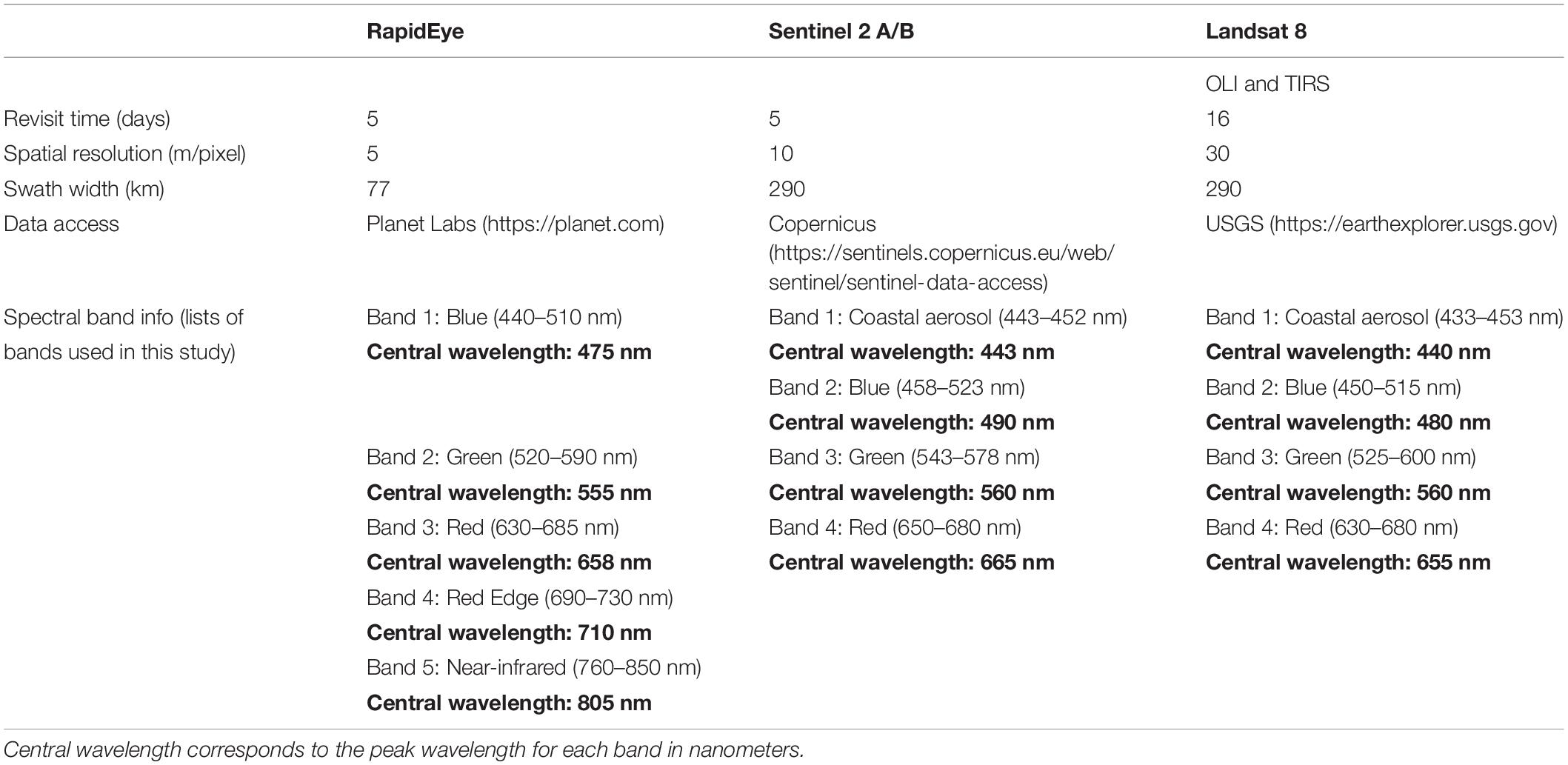
Table 1. Optical satellite specifications for RapidEye, Sentinel-2 A/B, and Landsat 8.

The Copernicus Sentinel-2A and Sentinel-2B missions were launched on June 23, 2015 and March 7, 2017, respectively, and are operated by the European Space Agency (ESA). Each instrument consists of 12 spectral bands and a swath width of 290 km, and a spatial resolution of 10 m. The Landsat 8 mission carrying the Operational Land Imager (OLI) and the Thermal Infrared Sensor (TIRS) is operated by the USGS and was launched on February 11, 2013. The OLI has 9 spectral bands and a swath width of 185 km. The spatial resolution of Landsat 8 is 30 m for the multispectral bands. Sentinel 2 A/B and Landsat 8 were used to calculate CDOM since they have the required bands to apply the Quasi-Analytical Algorithm (QAA) of Lee et al. (2002).

We utilize these sensors to examine and characterize the optical properties of both types of coastal plumes with the intent of separately classifying each type of plume. Since these plumes disperse after a day or two, a sensor that has a high spatial and temporal resolution is crucial (DiGiacomo et al., 2004).

A total of 40 RapidEye images were identified during these periods and separated into four groups (10 stormwater, 10 wastewater, 10 mixed (a combination of both), and 10 open ocean/no plume) and were then analyzed for differences in surface reflectance in five bands and other biochemical parameters such as turbidity and CDOM. We also utilize in situ data such as flow rate, precipitation, ENT, and plume color to differentiate between these groups. Supplementary Table 1 provides more detailed information on each RapidEye image and its output. RapidEye was used for all the outputs of spectral reflectance for consistency. Information on how the spectral reflectances values were extracted are in section “Spectral Profiles.”

Atmospheric Correction

For RapidEye, Sentinel-2, and Landsat-8 data, an atmospheric correction scheme was applied using ACOLITE software. The open-source program ACOLITE (Vanhellemont and Ruddick, 2018) was used to process these images with atmospheric corrections (Eq. 1) and to generate output parameters including remote sensing reflectance (Rrs), chlorophyll-a concentration (chla), CDOM (a443), suspended matter concentration, and turbidity (Vanhellemont, 2019a). ACOLITE can be downloaded from the GitHub repository for RapidEye imagery³ and Sentinel-2 and Landsat-8 imagery⁴. Atmospheric correction was calculated for all imagery using the following:

$\mathit{REF}\left(i\right)=\frac{\mathit{RAD}\left(i\right)\mathrm{\pi }{d}^2}{\mathit{ESI}(i)\cos {\mathrm{\theta }}_s}(1)$

where REF is the reflectance value for the top of atmosphere (TOA) reflectance, RAD is the radiance value, i is the number of the spectral band, d is the earth-sun distance at the day of acquisition in astronomical units (AU), ESI is the extraterrestrial solar irradiance, and θ_s is the solar zenith angle in degrees (90° – sun elevation). More information on calculating TOA reflectance and ESI values for each band can be found on the Planet Labs website⁵. REF is corrected using the Dark Spectrum Fitting (DSF) algorithm for the five RapidEye bands (Vanhellemont, 2019b). The DSF algorithm is an aerosol correction algorithm and is used to estimate surface reflectance (see text footnote 3). All imagery was atmospherically corrected using the DSF algorithm.

Remote Sensing Based Analyses

Spectral Profiles

We utilize a region of interest polygon (circle) to define the area of interest (AOI) for all RapidEye images with a size of 1.28 km² (51,076 pixels) to maintain consistency when examining spectral properties for different plume events. An example of the AOI is symbolized as a white circle in Figure 2. The surface reflectance values, after the atmospheric correction, were extracted from the AOI and were spatially averaged to obtain the mean surface reflectance value for each band in the AOI. The same process was done for all 10 events for each of the four groups.

FIGURE 2

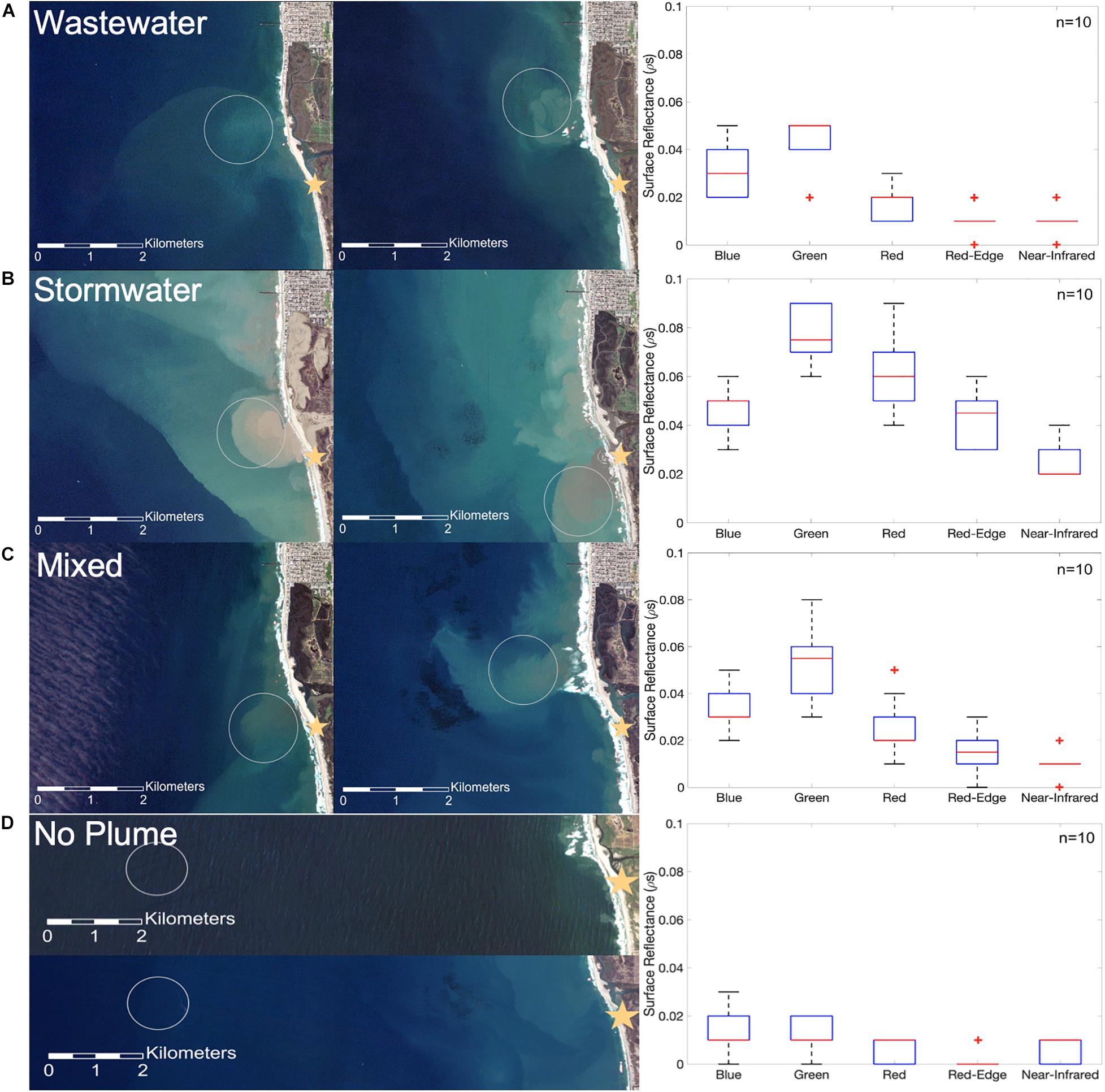
Figure 2. Surface Reflectances for (A) Wastewater, (B) Stormwater, (C) Mixed, and (D) No event/No Plume. Images are the true color imagery from RapidEye with AOI circled. Box plots are the surface reflectance values for each plume type (10 events per type). A yellow star denotes the Tijuana River mouth. (A) Wastewater Plume Events: on 1/24/19 (left image): 610 million gallons (MG) of raw wastewater (occurred on 1/18 and ended on 1/30). 12/11/18 (right image): 147.7 MG of raw wastewater (occurred on 12/11 and ended on 12/24). (B) Stormwater Plume Events: 12/7/18 (left image): precipitation amount was 1.07 inches (2.7 cm) on 12/6/18 and flow rate hourly mean was 158.3 cms. 1/28/10 (right image): precipitation amount was 0.07 inches (0.18 cm) on 1/26/10 and no data available for flow rate. (C) Mixed Plume Events: 2/9/17 (left image): 143 MG of raw wastewater (occurred on 2/6/17 and ended on 2/23/2017), precipitation amount on 2/7 was 0.19 inches (0.48 cm), and flow rate hourly mean was 2.4 cms. 1/24/16 (right image): 23.7 MG of raw wastewater (occurred on 1/16/16 and ended on 1/24/16), precipitation amount on 1/23/16 was 0.4 inches (1 cm), and flow rate hourly mean was 0.2 cms. (D) No Plume Events: 3/23/17 (top image) and 12/16/15 (bottom image): no wastewater or precipitation events for at least a month. The AOI is extracted offshore due to natural sedimentation near the coast, which may influence surface reflectance values. For each box plot, the median is shown by the red mark, the whiskers correspond to the maximum and minimum values, the red plus signs show the outliers outside of the 25–75 percentile range shown by the box.

Derived Turbidity

Turbidity is the measure of water clarity in a body of water. High turbidity is often due to high concentrations of suspended particles from sediments, CDOM, or algae and has units of Formazine Nephelometric Units (FNU) or Nephelometric Turbidity Unit (NTU). The bands that can detect turbidity are red, red-edge, or near-infrared (NIR) since turbidity has the optical properties of scattering light in these bands (Dogliotti et al., 2015; Hafeez et al., 2018). Turbidity is computed using the following equation (Nechad et al., 2009):

$T=\frac{A{\mathrm{\rho }}_w}{1-\frac{{\mathrm{\rho }}_w}{C}}(2)$

where T is the algorithm derived turbidity, ρw is the surface reflectance after atmospheric correction, and A and C are constant coefficients associated with inherent optical properties. Vanhellemont (2019b) shows excellent agreement from using RapidEye’s red and red-edge bands after comparing seven sites (sites in Northern California, North Sea, and the Irish Sea) of in situ turbidity with derived turbidity. We decided to use RapidEye’s red band for ρw since it gave the best results according to the Vanhellemont (2019b) study. We used the default A and C values, 247.10 and 0.1697, respectively, for the red band based on recommendations from Nechad et al. (2009) and Vanhellemont (2019b).

Derived Colored Dissolved Organic Matter

Colored dissolved organic matter is a yellow substance, gelbstoff, from the mixing of organic matter such as remains of plants and animals. High concentrations of CDOM arise from the breakdown of dead organisms and organic matter. The color of CDOM can range from yellow to brown in nearshore waters (Aurin et al., 2018). To calculate CDOM, we implement the Quasi-Analytical Algorithm (QAA) from Lee et al. (2002). Bands that are needed to calculate CDOM (a443) have a wavelength of 443, 490, 560, and 665 nm. Sentinel-2 A/B and Landsat 8 were used since they have all the required bands to derive CDOM. RapidEye has only one band from 410 to 510 nm (blue band) and may not give an estimate for CDOM. From the multistep process (shown in Supplementary Table 4), we obtain absorption outputs: a443, a490, a560, and a665. CDOM absorption can also be observed in the blue band since it absorbs in the UV and visible (blue light) spectrum range. The most recent updates to the QAA algorithm are in both version 5 (Lee et al., 2009) and version 6 (Lee et al., 2014) which incorporate Rrs (670 nm) (remote sensing reflectance in band 670 nm) since most sensors (MODIS, Sentinel-2, Landsat 8) have a band near this wavelength. ACOLITE applies either version 5 or version 6 depending on if Rrs (670nm) is less than 0.0015. Supplementary Table 4 displays the equations to calculate a443 (CDOM). CDOM is calculated for 5 stormwater, 5 wastewater, 5 mixed, and 5 open ocean/no plume events from the AOI using Landsat 8 and Sentinel 2 A/B imagery (Supplementary Table 3).

Water Quality in situ Data

The NOAA National Estuarine Research Reserve System (NERRS)⁶, a long-term monitoring program to protect estuarine ecosystems, has 28 stations across the United States collecting water quality, meteorological, nutrient, and pigment data. Each station is located near an estuary with an automatic sampler that collects data every 15 min (every 30 min prior to 2007). Two NOAA stations are used in this study, with one located at the mouth of the Tijuana River (Boca Rio: purple star in Figure 1) and the other inside the estuary (Oneonta Slough: light green star in Figure 1). Water quality parameters of interest are turbidity (FNU/NTU) and chlorophyll fluorescence (ug/L). The visual observations are also reported at each shore station including water color, water clarity, and human or animal activity (Supplementary Table 2). We used these visual observations to validate the plume color and water clarity observed from the true color imagery.

Wastewater spill data is from the City of San Diego (see text footnote 2) under Spill Reports, which provides the amount of wastewater spills and when the spills occurred. We also incorporate enterococcus (ENT) (CFU/100 mL) from The City of San Diego Public Utilities⁷ to check the bacteria levels during a wastewater or stormwater event. Bacteria levels of ENT that go above 100 CFU/100mL are deemed harmful by the EPA standards (see text footnote 1). ENT is commonly used as an indicator of harmful bacteria and viruses that can cause illnesses in swimmers and surfers (Schiff et al., 2016). These data are used to characterize and compare the impact of wastewater and stormwater plumes with respect to turbidity and ENT.

Precipitation and Flow Gauge Data

Precipitation data are acquired from NOAA⁸ from 2010 to 2019, which is collected at the precipitation station at the Brown Field Municipal Airport marked as the blue star in Figure 1. Precipitation values for all stormwater events were plotted using MATLAB and are shown in Supplementary Figure 2. The units for the daily precipitation amount are in inches. Flow gauge data is from the International Boundary & Water Commission (IBWC)⁹, whose station is marked as the green star in Figure 1. The units for flow rate are in cubic meters per second (cms) and the flow rate is the hourly mean of 12 h prior to the satellite acquisition time. We use the hourly mean for the 12-h window since the flow gauge station is located upstream on the river approximately 6.4 km from the river mouth.

Analyses and Comparison of Plumes

Plume Comparison Using Spectral Data and in situ Data

To compare spectral reflectance information for each plume type, we created a box plot for each band using all 10 events shown in Figure 2. Figure 2A is an example of two wastewater plumes coming out of the Tijuana River Mouth on January 24, 2019 (147 million gallons of wastewater) and December 7, 2019 (610 million gallons of wastewater). Figure 2B is an example of two stormwater plumes on December 7, 2018 (1.07 inches of precipitation) and January 28, 2010 (0.07 inches of precipitation). Figure 2C is an example of two mixed plumes on February 9, 2017 (0.19 inches of precipitation and 143 million gallons of wastewater) and January 24, 2016 (0.4 inches of precipitation and 23.7 million gallons of wastewater). Figure 2D is an example of no plume events on March 23, 2017 and December 16, 2015. For both events, there is no wastewater or precipitation amounts. We compared the ranges of the reflectance values for each band to observe spectral differences across all bands. A line graph of these surface reflectance values was plotted with ±1 standard deviation from the average spectral value for each plume type shown in Figure 3. Box plots of mean derived CDOM and turbidity from the AOI, and the in situ mean hourly flow rate and ENT (Supplementary Table 2) values were generated for each plume group. We implemented a one-way analysis of variance (ANOVA) test to determine if the means are different for each group.

FIGURE 3

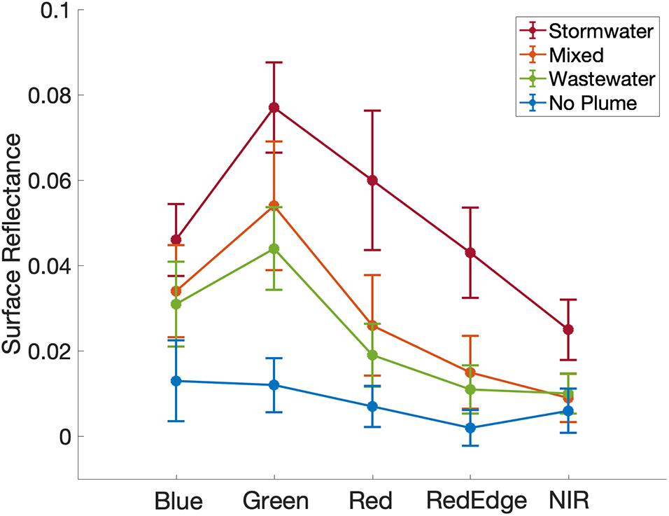
Figure 3. Line graph of surface reflectances for 10 stormwater plumes, 10 wastewater plumes, 10 mixed plumes, and 10 open ocean events. The y-axis indicates the surface reflectance values and the x-axis is the wavelength. The bounding bars are the ±1 standard deviation from the average spectral value.

Hierarchical Cluster Analysis and Principal Component Analyses

Two approaches were utilized to investigate how spectral data can be used to assess coastal plume classes. First, we applied a principal component analysis (PCA) (Jolliffe and Cadima, 2016) to our dataset of surface reflectance and derived turbidity values from the defined AOI. This was done directly on raw data (with the exception of averaging over an area of interest) to preserve variability in the dataset and account for interrelatedness of surface reflectance values between bands and because turbidity is derived from spectral information. PCA has been conducted on numerous studies of the natural and built environment in various capacities (Gašparović and Jogun, 2018; Judice et al., 2020) and is especially used for simplifying high dimensionality datasets and for classification applications. The principal components (PC1 and PC2) were then plotted to see whether groups of coastal plume classes were clearly clustered or not.

The second methodology applied here was the hierarchical cluster analysis (HCA) in a complete-linkage clustering approach (Revelle, 1979). The purpose of utilizing an alternate approach was to see if both modes of analysis would reinforce the observed spectrally dependent differentiation of coastal plume types. HCA performed in this study uses an agglomerative scheme that considers each sample as its own individual cluster. Clusters that are considered more similar (i.e., shortest distance) are then used to generate larger clusters. Previous work has demonstrated the utility of HCA on water quality classifications and aquatic properties (Brezonik et al., 2005; Kamble and Vijay, 2011; Reynolds and Stramski, 2019).

Both HCA and PCA utilized input data from 30 separate coastal plume events – 10 were considered “no plume” or open ocean, 10 were considered sewage spill plumes, and 10 were considered stormwater plumes. Pixels for the AOI were averaged for each of these events, the events are summarized in Supplementary Table 1.

Results

Plume Comparison Using Spectra Data of AOI (Surface Reflectance, Turbidity, and CDOM)

Figure 2A shows wastewater plume reflectance values ranged from low-medium reflectance in the blue to green bands and low reflectance in the red-NIR bands. Stormwater plumes had medium reflectance in the blue band, medium-high reflectance in the green to red-edge bands, and low-medium reflectance in the NIR shown in Figure 2B. The results show that the stormwater plumes have the highest reflectance in the green-red region (500–700 nm) which could potentially be due to increased sediment loading. Figure 2C shows there is considerable overlap of mixed plumes in the green and red bands, especially with both the stormwater and wastewater plumes only, indicating varying concentrations and extent of both wastewater and sediments shown. Wastewater and mixed plumes reflect mostly in the green band (500–600 nm) which may be due to CDOM or chlorophyll. Open ocean/no plume has the lowest reflectance across all wavelengths considered as shown in Figure 2D. Wastewater plumes are clearly separated from stormwater plumes in all five bands.

The line graph in Figure 3 shows the surface reflectances of 10 stormwater plumes, 10 wastewater plumes, 10 mixed plumes, and 10 open ocean/no plume events. Each plot represents the average reflectance value and the bounding bars indicate ±1 standard deviation. These surface reflectance values are shown in Supplementary Figure 1.

We conducted an HCA and a PCA on 30 independent plume images, where 10 images were associated with stormwater, 10 for wastewater, and 10 for open ocean/no plume events. Mixed plumes were excluded from this analysis because their spectral signature overlapped with wastewater plumes. As seen in Figure 4A, there are three primary branches that correspond with each of the coastal plume classes evaluated in this analysis: O (Open Ocean/No Plume – in red); WW (Wastewater – in green); and SW (Stormwater – in blue). Three of the open ocean samples (O8, O9, and O10) were clustered into the wastewater plumes branch, indicating that 27 out of 30 events were classified into their matching plume class (90% correct classification).

FIGURE 4

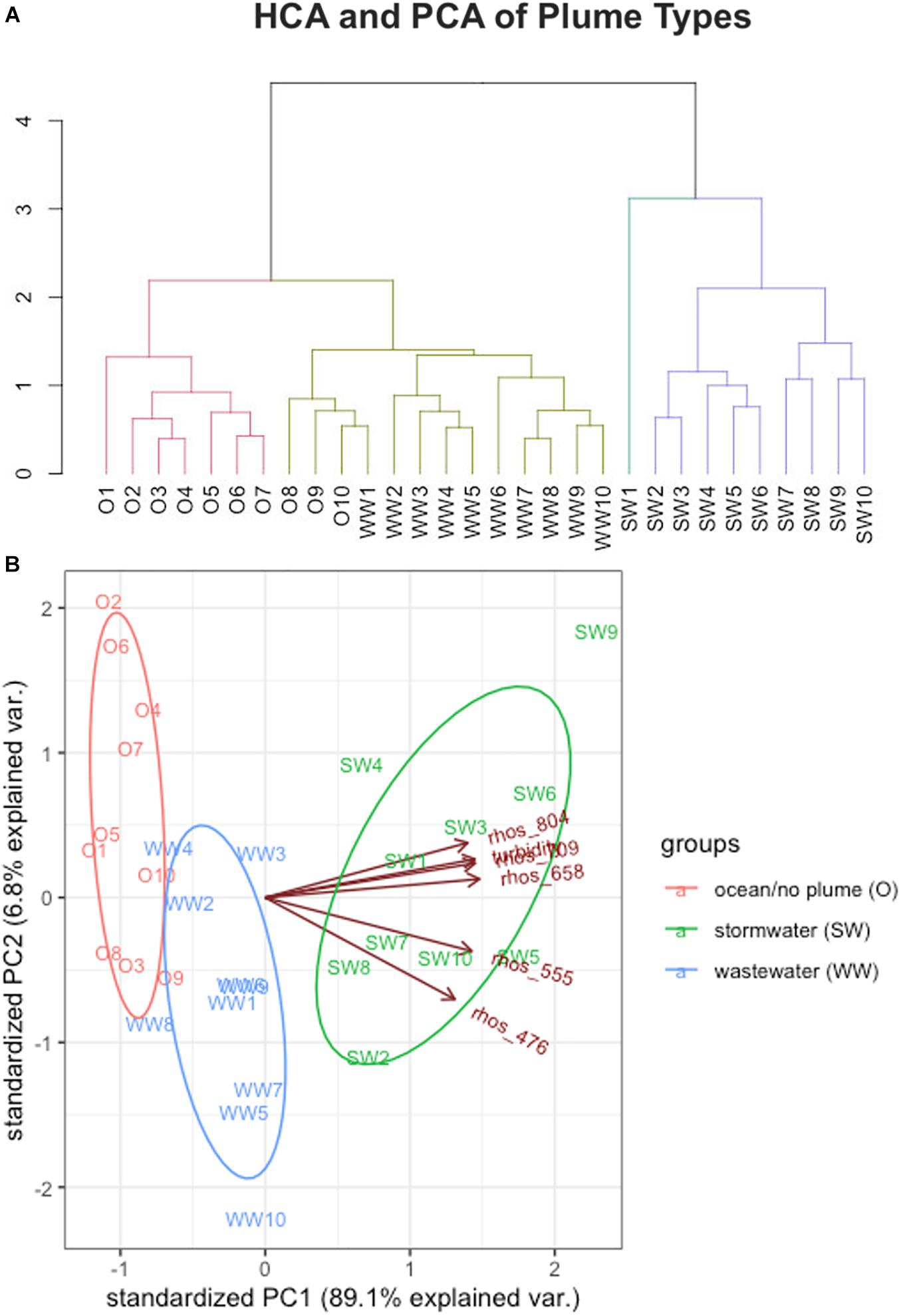
Figure 4. HCA and PCA Analysis. (A) A dendrogram tree from the HCA. (B) PCA result of PC1 on the x-axis, and PC2 on the y-axis. The arrows indicate the relative influence of the parameters used in the underlying data (surface reflectance and derived turbidity).

In the PCA analysis, (Figure 4B) we see two distinct groups [(1) Open Ocean/Wastewater and (2) Stormwater], differentiated across PC1, the component that accounts for the majority of the variance (89.1%) and less clear distinction across the y-axis/PC2 for open ocean and wastewater, with PC2 explaining about 6.8% of the variance. While O9 and O10 are in closest proximity to the WW samples, O3 a slightly closer than O8 is, which is a slight difference between HCA and PCA evaluations. PC1 and PC2 are plotted here to help evaluate the similarities and distributions in sample types relative to their classes.

We utilize the a443 parameter (Lee et al., 2002) from ACOLITE that derives CDOM to compare the CDOM concentrations between plume types. Figure 5A is the derived CDOM (a443) parameter from 5 stormwater, 5 wastewater, 5 mixed, and 5 open ocean/no plume events (Supplementary Table 3). Since CDOM can only be calculated using Landsat 8 and Sentinel 2 imageries, we were only able to acquire a limited number of these events for comparison. From Figure 5A, the mean CDOM values for our AOI ranged from 0.06 to 0.32 m^–1 (low CDOM) for open ocean/no plume, 0.3 to 0.59 m^–1 (low-medium CDOM) for wastewater, 0.39 to 0.96 m^–1 (medium-high CDOM) for mixed, and 0.98 to 2.1 m^–1 (high CDOM) for stormwater. The P-value from ANOVA test is 8.96e-6 for CDOM. CDOM has the 2nd highest variance compared to turbidity, ENT, and flow rate. Overall, we observed that the wastewater plumes have less CDOM compared to the stormwater plumes (Supplementary Table 3).

FIGURE 5

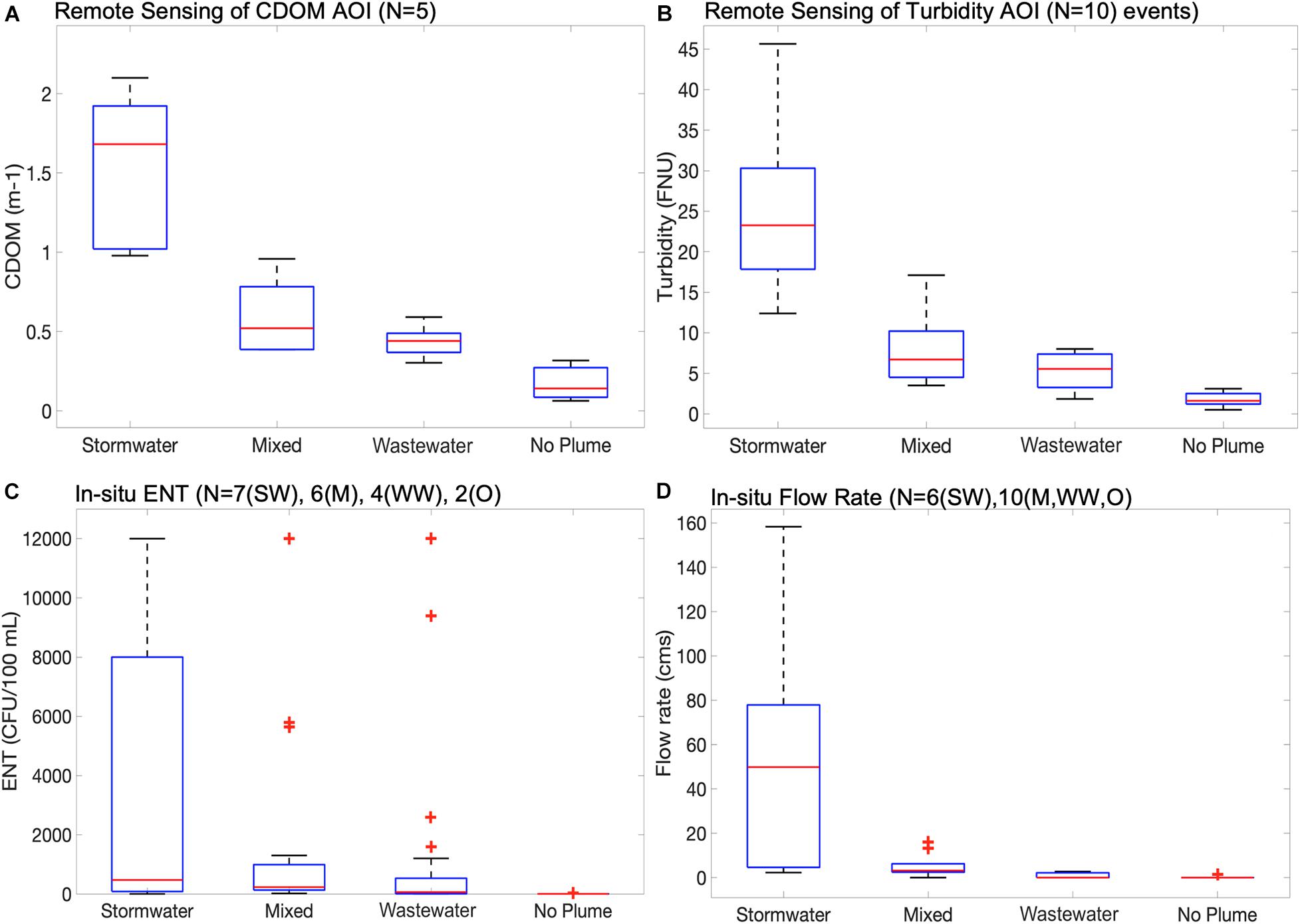
Figure 5. Box plots of CDOM and turbidity derived from remote sensing data, and ENT and flow rate from in situ measurements. (A) Mean derived CDOM from AOI (Lee et al., 2002) for 5 stormwater, 5 mixed, 5 wastewater, and 5 no plume events using Landsat 8 and Sentinel 2 A/B data (more information: Supplementary Table 3). (B) Mean derived turbidity from AOI (Nechad et al., 2009) for 10 stormwater, 10 wastewater, 10 mixed, and 10 no plume events using RapidEye data. (C) Enterococcus (ENT) counts for 7 stormwater, 6 mixed, 4 wastewater, and 2 no plume events (more information: Supplementary Table 2). (D) Mean flow rate from gauge station (Figure 1: green star) in cubic meters per second (cms) from 12 h prior to the satellite revisit time for 6 stormwater events and 10 wastewater, 10 mixed, and 10 no plume events). For each box plot, the median is shown by the red mark, the whiskers correspond to the maximum and minimum values, the red plus signs show the outliers outside of the 25–75 percentile range shown by the box.

Figure 5B shows derived turbidity (mean of AOI) from Eq. 2 for all four groups. The turbidity mean values ranges from 0.5 to 3.1 FNU (low turbidity) for open ocean/no plume, 1.83 to 8 FNU (low-medium turbidity) for wastewater, 3.5 to 17.1 FNU (medium-high turbidity) for mixed, and 12.38 to 45.65 FNU (high turbidity) for stormwater. In Figure 5B, we observed that turbidity existed for all 3 types of plume events. The P-value from ANOVA test is 3.24e-10 for turbidity. Turbidity has the highest variance compared to CDOM, ENT, and flow rate.

Plume Comparison Using in situ Data (Plume Color, Flow Rate, and ENT)

In situ water quality data was acquired from the water quality station monitoring reports for 7 stormwater, 6 mixed, 5 wastewater, and 2 open ocean/no plume events that match with our RapidEye imagery. There are several sampling locations for each event (Figure 1: offshore and shore stations). We extracted the station data that are within each plume or closest to the river mouth (more information: Supplementary Table 2). Figure 5C shows that the average ENT for the open ocean/no plume events is low (3.2 CFU/100 mL), wastewater average ENT is medium (890 CFU/100 mL), mixed average ENT is relatively high (1314.1 CFU/100 mL), and stormwater average ENT is high (3440.5 CFU/100 mL). The P-value from ANOVA test is 1.45e-4 for ENT.

We also see differences in plume color for wastewater and stormwater plumes. Wastewater plumes are green while stormwater plumes are brown based on the true color imagery (Supplementary Table 1). Mixed plumes are a combination of greenish-brown and open ocean/no plumes are dark blue in the imagery. Such color difference was also captured by the visual observations in the water quality station monitoring reports (offshore and shore stations in Figure 1) for the events in Supplementary Table 2. Wastewater events reported that the water color was green and included: sewage like odor, turbid water, and debris. Stormwater events reported that the water color was brown and included: turbid water, sewage like odor, debris, and detergent-like odor. Mixed events reported that the water color was green or brown and included: sewage like odor, water turbid, and foam present. Open ocean/no plume events reported that the water color was greenish-blue and no comments included in visual observations.

Figure 5D shows the hourly mean flow rate from the flow gauge station (green star) in Figure 1. Stormwater flow rates from events 1–4 (Supplementary Table 1) are missing since there are no data available during those dates. Flow rate includes all 10 events for wastewater, mixed, and open ocean/no plume events. Figure 5D shows that the flow rate values for open ocean/no plume range from 0.1 to 1.3 cms (low flow), 0 to 2.7 cms for wastewater (low flow), 0 to 16 cms for mixed (medium flow), and 2.2 to 158.3 cms for stormwater (high flow). The stormwater events typically exhibit relatively higher flow rates, which is consistent with being associated with precipitation events. The P-value from ANOVA test is 1.3e-4 for flow rate. ENT and flow rate have similar variances since these values are closer to the mean compared to turbidity and CDOM. Since all p-values from the ANOVA test for all parameters are less than the significance level of 0.05, we reject the null hypothesis that four groups have equal means.

Evaluation of Satellite-Derived Turbidity

Satellite-derived turbidity values for RapidEye were compared with those collected from in situ stations in the Tijuana River to assure the accuracy of the satellite measurements. It should be noted that in situ data for CDOM and spectral data were not available for evaluation. The in situ water quality stations are from the NOAA NERRS and are located at the mouth of the Tijuana River (Boca Rio: purple star in Figure 1) and inside the estuary (Oneonta Slough: light green star in Figure 1).

We compared the turbidity from water quality station at Oneonta Slough (Figure 6A) to the algorithm derived turbidity from 40 images listed in the Supplementary Table 1, including 10 wastewater events, 10 stormwater events, 10 mixed events, and 10 open ocean/no plume. We extracted a 3 × 3 pixel area surrounding the Oneonta Slough Station to compute the average derived turbidity. This average derived turbidity is compared with the in situ hourly average turbidity (4 of the 15-min turbidity values are averaged). The same methods were applied to the Boca Rio station (Figure 6B). The high peaks of turbidity from Figures 6A,B are from stormwater (SW) events, moderate values of turbidity are from wastewater (WW), and mixed (M) events, and low turbidity values are from open ocean/no plume events (O). Oneonta Slough has an R² of 0.94, and the Boca Rio station has an R² of 0.71 with a sample size of 40 for each station. Figures 6C,D are the regression line plots for the Oneonta Slough Station and Boca Rio Station, respectively.

FIGURE 6

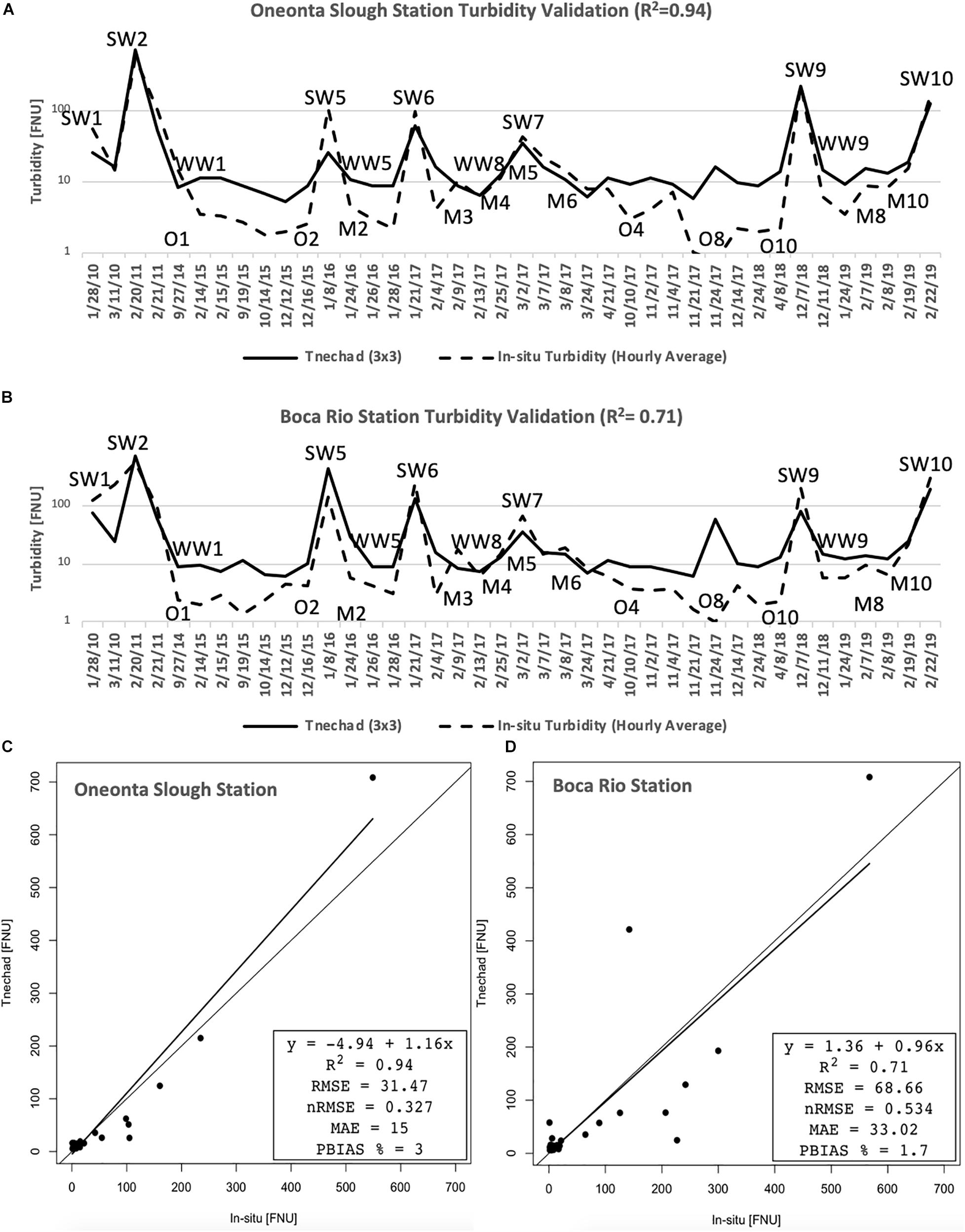
Figure 6. Turbidity validation at the (A) Oneonta Slough Station and (B) Boca Rio Station. (C,D) The regression plots for both stations. Both stations have 40 points each: 10 stormwater, 10 wastewater, 10 mixed, and 10 no plume events.

Discussion and Conclusion

Previous remote sensing studies focused on tracking, dispersal, detection, and impacts of stormwater plumes (Warrick et al., 2007; Lahet and Stramski, 2010; Svejkovsky et al., 2010; Brando et al., 2015; Holt et al., 2017). There are limited studies on remote sensing of wastewater plumes (DiGiacomo et al., 2004; Marmorino et al., 2010; Gierach et al., 2017; Trinh et al., 2017). However, no known studies have performed the classification of these plume types. Our study differentiated the wastewater and stormwater events based on the different characteristics presented in the plumes. These parameters include spectral profile, CDOM, turbidity, flow rate, plume color, and bacteria level (ENT).

Stormwater plumes reflectance values are consistent with other studies where we see highest reflectance values in the blue to red ranges (Hafeez et al., 2018; Wang et al., 2019). The wastewater plumes reflect most strongly in the green wavelength which shows similar reflectance signatures as CDOM and chlorophyll. Mixed events show a wide range of reflectance, which depends on a case by case basis on having “more stormwater” or “more wastewater” in the mixed plumes. Through conducting HCA and PCA of surface reflectance values, we were able to classify stormwater, wastewater, and open ocean/no plume in nearly all cases (90% success rate). HCA and PCA managed to cluster these events into 3 groups by finding similar surface reflectance values for each group. However, HCA misclassified three ocean samples to wastewater and PCA misclassified two wastewater samples to open ocean/no plume and one open ocean/no plume to wastewater. The majority of the samples show that wastewater and ocean (low-moderate reflectance in the visible) are more related to each other as compared to stormwater (high reflectance in the visible). This might be due to some open ocean/no plume events also having small concentrations of CDOM or chlorophyll, which reflects in the blue-green band ranges. Another issue may be the amount of wastewater and its varying concentration and properties that could influence the surface reflectance values. For example, the wastewater amounts range from 172,000 gallons to 610 million gallons. These wastewater events are also comprised of treated wastewater, untreated wastewater, or a combination of both (see text footnote 1). The plumes that were misclassified were WW4 and WW8 and we included the end times of each spill in Supplementary Table 1. There may have been less wastewater for WW4 since the reported spill ended 4 h prior to the satellite acquisition time. WW8 might have been less wastewater as well since it was in the middle date of a spill that lasted 17 days. The wastewater amount was significant (143 MG) but occurred throughout these days. Overall, the majority of the highest reflectances values were those with the highest reported wastewater amounts. There were higher amounts of CDOM in stormwater (0.98 to 2.1 m^–1) and lower CDOM values for wastewater (0.3 to 0.59 m^–1) (shown in Figure 5A). Mixed plumes are in-between ranging from 0.39 to 0.96 m^–1. Studies have shown variable concentrations of CDOM in wastewater plumes, which may be due to the dilution and transport of these plumes (Marmorino et al., 2010; Gierach et al., 2017).

Validation was only implemented for turbidity since no in situ data was available for reflectance or CDOM. Turbidity validation showed high correlations for both the Oneonta Slough (R² = 0.94) and Boca Rio (R² = 0.71) stations. The Oneonta Slough station obtained the best results due to the station being in quieter waters with low wave energy (in the estuary) compared to the Boca Rio station located at the river mouth. At the Boca Rio station there may be high energy waves which can fluctuate the turbidity values. In Vanhellemont (2019b), the turbidity deriving algorithm (Nechad et al., 2009) was validated for RapidEye in several sample sites with 84 smart Buoys and 129 USGS sites that matched with RapidEye imagery. The algorithm was able to achieve R² of 0.78 and 0.81 in the validation of these sites using the red band. Both Vanhellemont (2019b) and this study have shown that RapidEye imagery can be used to derive meaningful and accurate turbidity results based on the Nechad et al. (2009) algorithm.

Turbidity existed in our 3 water groups: stormwater, wastewater, and mixed (Figure 5B). Stormwater showed the highest turbidity (ranging from 12.38 to 45.65 FNU) out of all the groups due to the high amount of sediments in these plumes. Since mixed plumes are a combination of wastewater and stormwater, the average turbidity ranges from 3.5 to 17.1 FNU. Wastewater turbidity values are on the lower end ranging from 1.83 to 8 FNU. Open ocean/no plume has almost no turbidity ranging from 0.5 to 3.1 FNU. Flow rate (Figure 5D) showed a similar pattern as turbidity: high flow rate values for stormwater, low-medium flow rate for mixed, low flow rate for wastewater, and almost no flow rate for open ocean/no plume. High flow amounts are most common when there is runoff from precipitation which is why there are higher flow rates for stormwater events. Other studies have reported high flow rates (Corcoran et al., 2010; Holt et al., 2017) and turbidity (Washburn et al., 2003) for stormwater plumes due to increases in sediments, dirt, oil, and other pollutants. For wastewater, results found that the flow rate is low which may be due to the gauge not being able to accurately estimate the flow. A report from IBWC¹⁰ found that the flow gauge accuracy is ± 5% and is not able to detect low flow rates. It is unclear why the wastewater flow rate is almost undetected since some spills report millions of gallons of wastewater discharged into the Tijuana River. The IBWC report mentions that this is due to silt and solid sediments in the river.

Plume color differences are seen in the true-color imagery: wastewater plume is green while the stormwater plume is brown. Mixed plumes are a combination of both (greenish-brown) and open ocean/no plume is dark blue. The water quality station monitoring reports observed that wastewater plumes are green, stormwater plumes are brown, mixed plumes are green or brown, and no plume waters are greenish-blue. Depending on whether a wastewater spill is treated (less ENT), stormwater plumes often result in high ENT since this is an unregulated non-point source. This is shown in Figure 5C with stormwater showing high ENT (average: 3440.5 CFU/100 mL) for reported events while wastewater showed lower ENT (average: 890 CFU/100 mL). The average ENT for mixed was 1314.1 CFU/100 mL and for open ocean/no plume was 3.2 CFU/100 mL.

We depend primarily on spectral data from RapidEye, which is highly limited in terms of spectral information but still useful enough to help classify between plumes at a reasonably good rate (90% correct). The uncertainties with utilizing remote sensing to study these optically complex waters come from variations in CDOM, chlorophyll-a, sun glint, bottom reflectance, and suspended sediments (Trinh, et al. 2017). Several studies (Kahru et al., 2012; Dogliotti et al., 2015; Ruddick et al., 2016; Trinh et al., 2017; Zheng and DiGiacomo, 2017; Vanhellemont, 2019a) have shown challenges in determining accurate chlorophyll-a concentrations in these optically complex waters. This is due to increases in CDOM and sediments near the coast. In this study, CDOM in stormwater plumes may be overestimated due to an increase in suspended sediment particles. However, without a more complete in situ data archive, we are unable to validate these parameters, such as CDOM and surface reflectance. Some of the limitations can be addressed by looking at more detailed spectral profiles, such as what might be offered by Landsat 8 and Sentinel-2 which we were only able to use in a limited way in this study. There are also opportunities to do data fusion or downscale by combining Landsat 8 and Sentinel-2 with RapidEye and PlanetScope, which might provide us more opportunity to address tradeoffs between spectral, temporal, and spatial resolutions. Another essential aspect to consider is understanding the hydrodynamics of wastewater plumes once they enter the ocean since there is little known on the residence time and dilution rates of wastewater.

It is also crucial to understand where these point and non-point sources are originating from. An example of a point source is a wastewater spill since it can be traced back to the wastewater treatment effluent. Stormwater plumes are a non-point source since this runoff can come from a variety of sources. A report from the City of San Diego¹¹ found that there are several potential non-point sources in this region such as agricultural operations, erosion due to unimproved roadways, homeless encampments, and natural sources of sediment. Moreover, since this watershed is both on the U.S-Mexico border, there are also pollutants from Mexico that contribute to this runoff. It is important to understand the origin of these sources and classify them in order to regulate harmful pollutants entering our waterways. In situ sampling in combination with remote sensing is necessary to tackle these complex problems and protect public health and the marine environment. Wastewater spills are becoming more common due to an increasing amount of people living in the Tijuana area; our techniques can be applied in order to help coastal managers detect and classify plume types in areas where there is less extensive monitoring of water quality.

Data Availability Statement

The raw data supporting the conclusions of this article will be made available by the authors, without undue reservation.

Author Contributions

JL, BH, and CL provided the guidance on designing and planning the study. All authors contributed and approved the final version of the manuscript.

Funding

This work was funded by the NASA Minority University Research and Education Project (MUREP) Institutional Research Opportunity under Grant (NNX15AQ06A). This work was performed at the California State University, Los Angeles and the Jet Propulsion Laboratory, California Institute of Technology, under contract with the National Aeronautics and Space Administration. The NASA DIRECT-STEM program was the primary support for this research.

Conflict of Interest

The authors declare that the research was conducted in the absence of any commercial or financial relationships that could be construed as a potential conflict of interest.

Acknowledgments

We would like to acknowledge Planet Labs for allowing access to RapidEye imagery for this study from the Education and Research Program and the Open California Program.

Supplementary Material

The Supplementary Material for this article can be found online at: https://www.frontiersin.org/articles/10.3389/fenvs.2020.599030/full#supplementary-material

Footnotes

1. ^ https://www.epa.gov/sites/production/files/2015-10/documents/rwqc2012.pdf
2. ^ http://www.waterboards.ca.gov/sandiego/water_issues/programs/tijuana_river_valley_ strategy/sewage_issue.html
3. ^ https://github.com/acolite/acolite_mr/
4. ^ https://github.com/acolite/acolite
5. ^ https://www.planet.com/products/satellite-imagery/files/160625-RapidEye%20Image-Product-Specifications.pdf
6. ^ http://cdmo.baruch.sc.edu
7. ^ https://www.sandiego.gov/public-utilities/sustainability/ocean-monitoring/data/south-bay
8. ^ https://www.ncdc.noaa.gov/orders/qclcd/
9. ^ https://www.ibwc.gov/Water_Data/Index.html
10. ^ https://www.ibwc.gov/Files/Report_Trans_Bypass_Flows_Tijuana_033117.pdf
11. ^ https://www.sandiego.gov/sites/default/files/legacy/stormwater/pdf/TJR_WaterQualityImprovementPlan_021715.pdf

References

Ackerman, D., and Weisberg, S. B. (2003). Relationship between rainfall and beach bacterial concentrations on Santa Monica Bay beaches. J. Water Health 1, 85–89. doi: 10.2166/wh.2003.0010

CrossRef Full Text | Google Scholar

Arnold, B. F., Schiff, K. C., Ercumen, A., Benjamin-Chung, J., Steele, J. A., and Griffith, J. F. (2017). Acute illness among surfers after exposure to seawater in dry-and wet-weather conditions. Am. J. Epidemiol. 186, 866–875. doi: 10.1093/aje/kwx019

PubMed Abstract | CrossRef Full Text | Google Scholar

Aurin, D., Mannino, A., and Lary, D. J. (2018). Remote sensing of CDOM, CDOM spectral slope, and dissolved organic carbon in the global ocean. Appl. Sci. 8:2687. doi: 10.3390/app8122687

PubMed Abstract | CrossRef Full Text | Google Scholar

Bay, S., Jones, B. H., Schiff, K., and Washburn, L. (2003). Water quality impacts of stormwater discharges to Santa Monica Bay. Mar. Environ. Res. 56, 205–223. doi: 10.1016/S0141-1136(02)00331-8

CrossRef Full Text | Google Scholar

Brando, V. E., Braga, F., Zaggia, L., Giardino, C., Bresciani, M., and Matta, E. (2015). High-resolution satellite turbidity and sea surface temperature observations of river plume interactions during a significant flood event. Ocean Sci. 11:909. doi: 10.5194/os-11-1-2015

CrossRef Full Text | Google Scholar

Brezonik, P., Menken, K. D., and Bauer, M. (2005). Landsat-based remote sensing of lake water quality characteristics, including chlorophyll and colored dissolved organic matter (CDOM). Lake Reserv. Manag. 21, 373–382. doi: 10.1080/07438140509354442

CrossRef Full Text | Google Scholar

Caron, D. A., Gellene, A. G., Smith, J., Seubert, E. L., Campbell, V., and Sukhatme, G. S. (2017). Response of phytoplankton and bacterial biomass during a wastewater effluent diversion into nearshore coastal waters. Estuar., Coast. Shelf Sci. 186, 223–236. doi: 10.1016/j.ecss.2015.09.013

CrossRef Full Text | Google Scholar

Corcoran, A. A., Reifel, K. M., Jones, B. H., and Shipe, R. F. (2010). Spatiotemporal development of physical, chemical, and biological characteristics of stormwater plumes in Santa Monica Bay, California (USA). J. Sea Res. 63, 129–142. doi: 10.1016/j.seares.2009.11.006

CrossRef Full Text | Google Scholar

Devlin, M. J., Petus, C., Da Silva, E., Tracey, D., Wolff, N. H., and Waterhouse, J. (2015). Water quality and river plume monitoring in the Great Barrier Reef: an overview of methods based on ocean colour satellite data. Remote Sens. 7, 12909–12941. doi: 10.3390/rs71012909

CrossRef Full Text | Google Scholar

DiGiacomo, P. M., Washburn, L., Holt, B., and Jones, B. H. (2004). Coastal pollution hazards in southern California observed by SAR imagery: stormwater plumes, wastewater plumes, and natural hydrocarbon seeps. Mar. Pollu. Bull. 49, 1013–1024. doi: 10.1016/j.marpolbul.2004.07.016

PubMed Abstract | CrossRef Full Text | Google Scholar

Dogliotti, A. I., Ruddick, K. G., Nechad, B., Doxaran, D., and Knaeps, E. (2015). A single algorithm to retrieve turbidity from remotely-sensed data in all coastal and estuarine waters. Remote Sens. Environ. 156, 157–168. doi: 10.1016/j.rse.2014.09.020

CrossRef Full Text | Google Scholar

Gašparović, M., and Jogun, T. (2018). The effect of fusing Sentinel-2 bands on land-cover classification. Int. J. Remote Sens. 39, 822–841. doi: 10.1080/01431161.2017.1392640

CrossRef Full Text | Google Scholar

Gierach, M. M., Holt, B., Trinh, R., Pan, B. J., and Rains, C. (2017). Satellite detection of wastewater diversion plumes in Southern California. Estuar. Coast. Shelf Sci. 186, 171–182. doi: 10.1016/j.ecss.2016.10.012

CrossRef Full Text | Google Scholar

Hafeez, S., Wong, M. S., Abbas, S., Kwok, C. Y., Nichol, J., Lee, K. H., et al. (2018). Detection and monitoring of marine pollution using remote sensing technologies. Monitor. Mar. Pollut. 2018, 81657. doi: 10.5772/intechopen.81657

CrossRef Full Text | Google Scholar

Holt, B., Trinh, R., and Gierach, M. M. (2017). Stormwater runoff plumes in the Southern California Bight: A comparison study with SAR and MODIS imagery. Marine Pollution. 118, 141–154. doi: 10.1016/j.marpolbul.2017.02.040

PubMed Abstract | CrossRef Full Text | Google Scholar

Jolliffe, I. T., and Cadima, J. (2016). Principal component analysis: a review and recent developments. Philos. Transac. R. Soc. A 374:20150202. doi: 10.1098/rsta.2015.0202

PubMed Abstract | CrossRef Full Text | Google Scholar

Judice, T. J., Widder, E. A., Falls, W. H., Avouris, D. M., Cristiano, D. J., and Ortiz, J. D. (2020). Field−validated detection of Aureoumbra lagunensis brown tide blooms in the Indian River Lagoon, Florida using Sentinel−3A OLCI and ground−based hyperspectral spectroradiometers. GeoHealth 4, e2019GH000238. doi: 10.1029/2019GH000238

PubMed Abstract | CrossRef Full Text | Google Scholar

Kahru, M., Kudela, R. M., Manzano-Sarabia, M., and Mitchell, B. G. (2012). Trends in the surface chlorophyll of the California Current: Merging data from multiple ocean color satellites. Deep Sea Res. 77, 89–98. doi: 10.1016/j.dsr2.2012.04.007

CrossRef Full Text | Google Scholar

Kamble, S. R., and Vijay, R. (2011). Assessment of water quality using cluster analysis in coastal region of Mumbai. India. Environ. Monitor. Assess. 178, 321–332. doi: 10.1007/s10661-010-1692-0

PubMed Abstract | CrossRef Full Text | Google Scholar

Lahet, F., and Stramski, D. (2010). MODIS imagery of turbid plumes in San Diego coastal waters during rainstorm events. Remote Sens. Environ. 114, 332–344. doi: 10.1016/j.rse.2009.09.017

CrossRef Full Text | Google Scholar

Lee, Z. P., Lubac, B., and Werdell, J. (2014). Update of the Quasi-Analytical Algorithm (QAA_v6). International Ocean Color Group Software Report,. http://www.ioccg.org/groups/Software_OCA/QAA_v6_2014209.pdf

Google Scholar

Lee, Z., Carder, K. L., and Arnone, R. A. (2002). Deriving inherent optical properties from water color: a multiband quasi-analytical algorithm for optically deep waters. Appl. Opt. 41, 5755–5772. doi: 10.1364/ao.41.005755

PubMed Abstract | CrossRef Full Text | Google Scholar

Lee, Z., Lubac, B., Werdell, J., and Arnone, R. (2009). An update of the quasi-analytical algorithm (QAA_v5). International Ocean Color Group Software Report, 1-9. https://www.ioccg.org/groups/Software_OCA/QAA_v5.pdf

Google Scholar

Marmorino, G. O., Smith, G. B., Miller, W. D., and Bowles, J. (2010). Detection of a buoyant coastal wastewater discharge using airborne hyperspectral and infrared imagery. J. Appl. Remote Sens. 4:043502. doi: 10.1117/1.3302630

CrossRef Full Text | Google Scholar

Nechad, B., Ruddick, K. G., and Neukermans, G. (2009). Calibration and validation of a generic multisensor algorithm for mapping of turbidity in coastal waters. Remote Sens. Ocean, Sea Ice Large Water Reg. 7473:74730H.

Google Scholar

Nezlin, N. P., and DiGiacomo, P. M. (2005). Satellite ocean color observations of stormwater runoff plumes along the San Pedro Shelf (southern California) during 1997–2003. Contin. Shelf Res. 25, 1692–1711. doi: 10.1016/j.csr.2005.05.001

CrossRef Full Text | Google Scholar

Nezlin, N. P., DiGiacomo, P. M., Diehl, D. W., Jones, B. H., Johnson, S. C., and Mengel, M. J. (2008). Stormwater plume detection by MODIS imagery in the southern California coastal ocean. Estuar. Coast. Shelf Sci. 80, 141–152. doi: 10.1016/j.ecss.2008.07.012

CrossRef Full Text | Google Scholar

Nezlin, N. P., Weisberg, S. B., and Diehl, D. W. (2007). Relative availability of satellite imagery and ship-based sampling for assessment of stormwater runoff plumes in coastal southern California. Estuar. Coast. Shelf Sci. 71, 250–258. doi: 10.1016/j.ecss.2006.07.016

CrossRef Full Text | Google Scholar

Reifel, K. M., Johnson, S. C., DiGiacomo, P. M., Mengel, M. J., Nezlin, N. P., and Warrick, J. A. (2009). Impacts of stormwater runoff in the Southern California Bight: Relationships among plume constituents. Cont. Shelf Res. 29, 1821–1835. doi: 10.1016/j.csr.2009.06.011

CrossRef Full Text | Google Scholar

Revelle, W. (1979). Hierarchical cluster analysis and the internal structure of tests. Multivar. Behav. Res. 14, 57–74. doi: 10.1207/s15327906mbr1401_4

CrossRef Full Text | Google Scholar

Reynolds, R. A., and Stramski, D. (2019). Optical characterization of marine phytoplankton assemblages within surface waters of the western Arctic Ocean. Limnol. Oceanogr. 64, 2478–2496. doi: 10.1002/lno.11199

PubMed Abstract | CrossRef Full Text | Google Scholar

Ruddick, K., Vanhellemont, Q., Dogliotti, A., Nechad, B., Pringle, N., and Van der Zande, D. (2016). “New opportunities and challenges for high resolution remote sensing of water colour,” in Proceedings of the Ocean Optics XXIII, (Victoria, BC), 23–28.

Google Scholar

Schiff, K., Griffith, J., Steele, J., Arnold, B., Ercumen, A., and Benjamin-Chung, J. (2016). The surfer health study: a three-year study examining illness rates associated with surfing during wet weather. SCCWRP Technol. Rep. 2016:943.

Google Scholar

Seegers, B. N., Teel, E. N., Kudela, R. M., Caron, D. A., and Jones, B. H. (2017). Glider and remote sensing observations of the upper ocean response to an extended shallow coastal diversion of wastewater effluent. Estuar. Coast. Shelf Sci. 186, 198–208. doi: 10.1016/j.ecss.2016.06.019

CrossRef Full Text | Google Scholar

Svejkovsky, J., Nezlin, N. P., Mustain, N. M., and Kum, J. B. (2010). Tracking stormwater discharge plumes and water quality of the Tijuana River with multispectral aerial imagery. Estuar. Coast. Shelf Sci. 87, 387–398. doi: 10.1016/j.ecss.2010.01.022

CrossRef Full Text | Google Scholar

Trinh, R. C., Fichot, C. G., Gierach, M. M., Holt, B., Malakar, N. K., and Hulley, G. (2017). Application of Landsat 8 for monitoring impacts of wastewater discharge on coastal water quality. Front. Mar. Sci. 4:329. doi: 10.3389/fmars.2017.00329

CrossRef Full Text | Google Scholar

Vanhellemont, Q. (2019a). Adaptation of the dark spectrum fitting atmospheric correction for aquatic applications of the Landsat and Sentinel-2 archives. Remote Sens. Environ. 225, 175–192. doi: 10.1016/j.rse.2019.03.010

CrossRef Full Text | Google Scholar

Vanhellemont, Q. (2019b). Daily metre-scale mapping of water turbidity using CubeSat imagery. Opt. Exp. 27, A1372–A1399. doi: 10.1364/OE.27.0A1372

PubMed Abstract | CrossRef Full Text | Google Scholar

Vanhellemont, Q., and Ruddick, K. (2018). Atmospheric correction of metre-scale optical satellite data for inland and coastal water applications. Remote Sens. Environ. 216, 586–597. doi: 10.1016/j.rse.2018.07.015

CrossRef Full Text | Google Scholar

Wang, D., Ma, R., Xue, K., and Loiselle, S. A. (2019). The assessment of Landsat-8 OLI atmospheric correction algorithms for inland waters. Remote Sens. 11:169. doi: 10.3390/rs11020169

CrossRef Full Text | Google Scholar

Warrick, J. A., DiGiacomo, P. M., Weisberg, S. B., Nezlin, N. P., Mengel, M., and Jones, B. H. (2007). River plume patterns and dynamics within the Southern California Bight. Cont. Shelf Res. 27, 2427–2448. doi: 10.1016/j.csr.2007.06.015

CrossRef Full Text | Google Scholar

Washburn, L., McClure, K. A., Jones, B. H., and Bay, S. M. (2003). Spatial scales and evolution of stormwater plumes in Santa Monica Bay. Mar. Environ. Res. 56, 103–125. doi: 10.1016/S0141-1136(02)00327-6

CrossRef Full Text | Google Scholar

Zheng, G., and DiGiacomo, P. M. (2017). Uncertainties and applications of satellite-derived coastal water quality products. Prog. Oceanogr. 159, 45–72. doi: 10.1016/j.pocean.2017.08.007

CrossRef Full Text | Google Scholar