Predicting the Number of Days With Visibility in a Specific Range in Warsaw (Poland) Based on Meteorological and Air Quality Data

Introduction

The effects of anthropogenic air pollution are discussed for years (Schedling, 1967; Saikawa et al., 2017; Kinney, 2018; Grewling et al., 2019; Makra, 2019). Visibility, an indicator of atmospheric transparency, refers to the visual range that distant objects can be clearly discerned (Li et al., 2019). Visibility is an atmospheric parameter, which can serve as a visual index for air quality (Kuo et al., 2013). Generally, visibility is the “distance at which the contrast of a given object with respect to its background is just equal to the contrast threshold of an observer” (WMO, 2015). It can also be defined as the clearness with which objects stand out from their backgrounds or other objects and how far people can see and how well they can identify objects (Bennett, 1930; Wooten and Hammond, 2002). Thus, a reduction in visibility is not simply fewer colors. On polluted days, however, the sky will appear white or grayish, and there is diminished contrast, making it difficult to discern the contours and details of objects (Ding et al., 2020). Many studies were made to evaluate the relationship between air pollution and visibility (Hyslop, 2009; Majewski et al., 2015; Qu et al., 2020). The impairment of visibility is primarily attributed to the scattering and absorption of visible light by particulate matter (PM). As the number of particulate of PM and selected PM components (e.g., black carbon) increases, more light is absorbed and scattered, resulting in less clarity, color, and visual range (Latha and Badarinath, 2003). Therefore, visibility at urban sites is mainly shaped by the emission of PM and PM precursors from anthropogenic sources like road traffic, combustion of fossil fuels, municipal solid waste treatment, and industry (Tsai et al., 2007; Deng et al., 2008; Zhao et al., 2011; Fajardo et al., 2013; Majewski et al., 2014; Zhuang et al., 2014).

Forecasting visibility is a complex task due to the multitude of parameters and nonlinear relations between these parameters. The statistical models which are currently used in the prediction of visibility have limited capabilities (Madan et al., 2000; Zhang et al., 2017; So et al., 2018; Dietz et al., 2019). We decided to use a classification model to make our forecast of visibility. We used multidimensional logistic regression since it allows us to assess the impact of a given variable on visibility without any additional calculations and the need for implementation of complex numerical algorithms (Hosmer et al., 2013). Although it is not easy to implement visibility–air quality interactions in the model, multiple outputs can be combined to improve visibility forecasting. Our solution allows the identification of visibility values in as many as four classes, taking into account different meteorological conditions and air quality measures (including the concentration of PM), which have not been analyzed in such scope before. Using the designated logistic models, cumulative empirical distributions of selected independent variables were identified, which was the basis for the development of their Monte Carlo generators. The obtained tool makes it possible to model the number of days with the visibility value within the appropriate range, which has not been analyzed in detail so far.

Generally, there is a lack of studies concerning the problem of visibility and air pollution in Poland since the air quality in Poland is one of the lowest in Europe (EEA, 2019). The air pollution in Poland is mainly caused by the emission from road traffic, industry, and energy production (Pastuszka et al., 2003; Rogula-Kozłowska et al., 2013; Błaszczak et al., 2016; KOBIZE, 2019). The impact of air quality in Poland can be seen in the scale of the whole of Europe (Spindler et al., 2010; Rogula-Kozłowska et al., 2014; Leoni et al., 2018); hence, monitoring of air quality including atmospheric visibility is very important. However, the visibility is monitored only at 15 places in Poland (PANSA, 2020), i.e., one place per over 20,000 km². This proves that the crucial point is the development of the methodology of forecast visibility which is based on historical data.

Here we presented an original model with the consistent methodological approach and assumptions. This approach to the visibility forecast can be successful in application to the analysis of publicly available data concerning many sites around the world.

Materials and Methods

Model Overview

The workflow of our original visibility forecast model is shown in Figure 1.

FIGURE 1

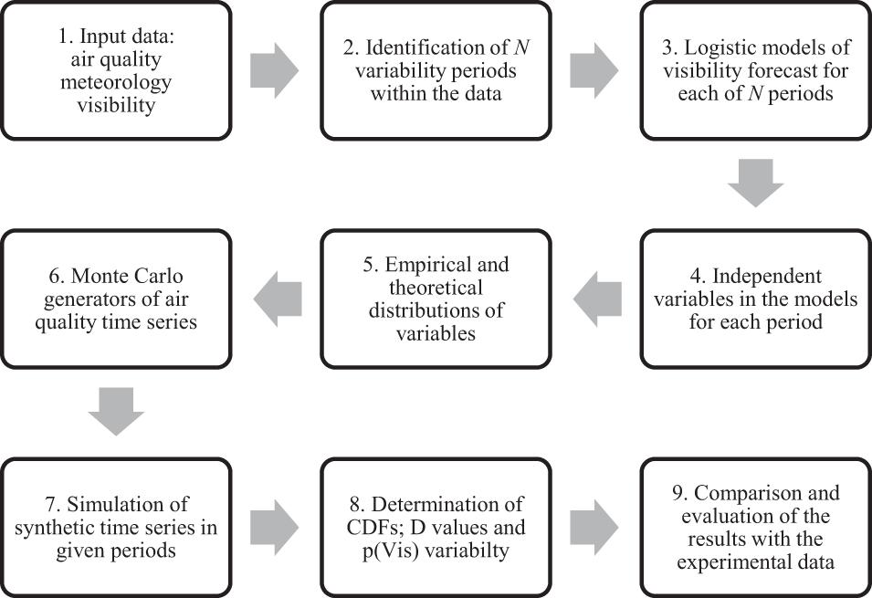
Figure 1. The workflow of determination of probabilistic model of simulation of visibility (Vis).

Air Quality and Meteorological Observations

The information used in the study came from the period between 2004 and 2013. We used data from three different monitoring stations located in the southern part of Warsaw, the capital of Poland. Their location is shown in Supplementary Figure 1. The air quality data were from the monitoring station MzWarWokalna located at 52.160772N, 21.033819E. We used 1-h average concentrations of sulfur dioxide (SO₂), carbon monoxide (CO), ozone (O₃), nitrogen dioxide (NO₂), and PM₁₀, monitored via pulsed fluorescence, infrared absorption, absorption of ultraviolet light, chemiluminescence, and a β-gauge automated particle sampler, respectively. The daily, arithmetic mean of 24 1-h concentrations was calculated for this study. The meteorological parameters were recorded at the Ursynów-SGGW station (52.160810N, 21.045681E). The meteorological data covered 24-h averaged data about air temperature $T\left[{}^{\circ }\mathrm{C}\right]$, solar irradiance $S\left[\frac{\text{W}}{{\text{m}}^2}\right]$, precipitation P[mm], and wind velocity $V\left[\frac{\text{m}}{\text{s}}\right]$. All the meteorological measurements were done according to the procedures of the Polish Institute of Meteorology and Water Management, National Research Institute (IMGW-PIB). The visibility was measured at the Warsaw Chopin Airport weather station (52.162876N, 20.961125E) with the use of a visibility meter equipped with an atmospheric phenomenon detector—Vaisala FS11 (wavelength 875 nm). It performed the functions of a visibility meter using light dispersion measurements and an atmospheric phenomenon detector with a measurement range from 10 to 50 km. The data (1-h values) were shared by the IMGW-PIB. For the whole research period, the 87,634 1-h values were obtained and a daily mean was calculated as for air quality data. We are then aware that during rain phenomena, the instrument FS11 is measuring beam attenuation due to scattering processes and is not physically taking absorption, e.g., by water vapor into account. The manufacturer claims that the response of the FS11 has been tested, evaluated, and 25 times verified with a transmissometer including a visible light band emitter at different locations around the world. Therefore, the absorption effect is covered to a certain extent, according to the manufacturer. We see the need of further research, aimed at a detailed analysis of visual range changes and precipitation.

The datasets were validated before the usage. The meteorological equipment was daily calibrated and validated by the personnel of the SGGW-WULS. The air quality data, before the publication in the archive of the Chief Inspectorate for Environmental Protection, are cross-checked and validated. The quality of the visibility data was constantly checked by the personnel at the Warsaw Chopin Airport since it determines the safety of the operation of the airport. As a result of these data quality control procedures, all the data which were outlier were removed by the respective services.

In the summer period (May–August), the median of all daily values of visibility in each month Vis(p = 0.50) has the highest value and is in the range 28.8–30.8 km, while in the winter period (November–February), the monthly visibility was the lowest and almost constant (in the range of 0.5 km). The visibility in the mid-period (March–April and September–October) has the highest change (from 13.4 to 28.8 km). Similar monthly trends are also observed for the Vis(p = 0.05) and Vis(p = 0.95). According to these observations and results of clustering data points (Figure 2), we divided the year into three periods (i.e., N = 3): (I) November–February, (II) March–April and September–October, and (III) May–August, which we analyzed separately (Supplementary Figure 2).

FIGURE 2

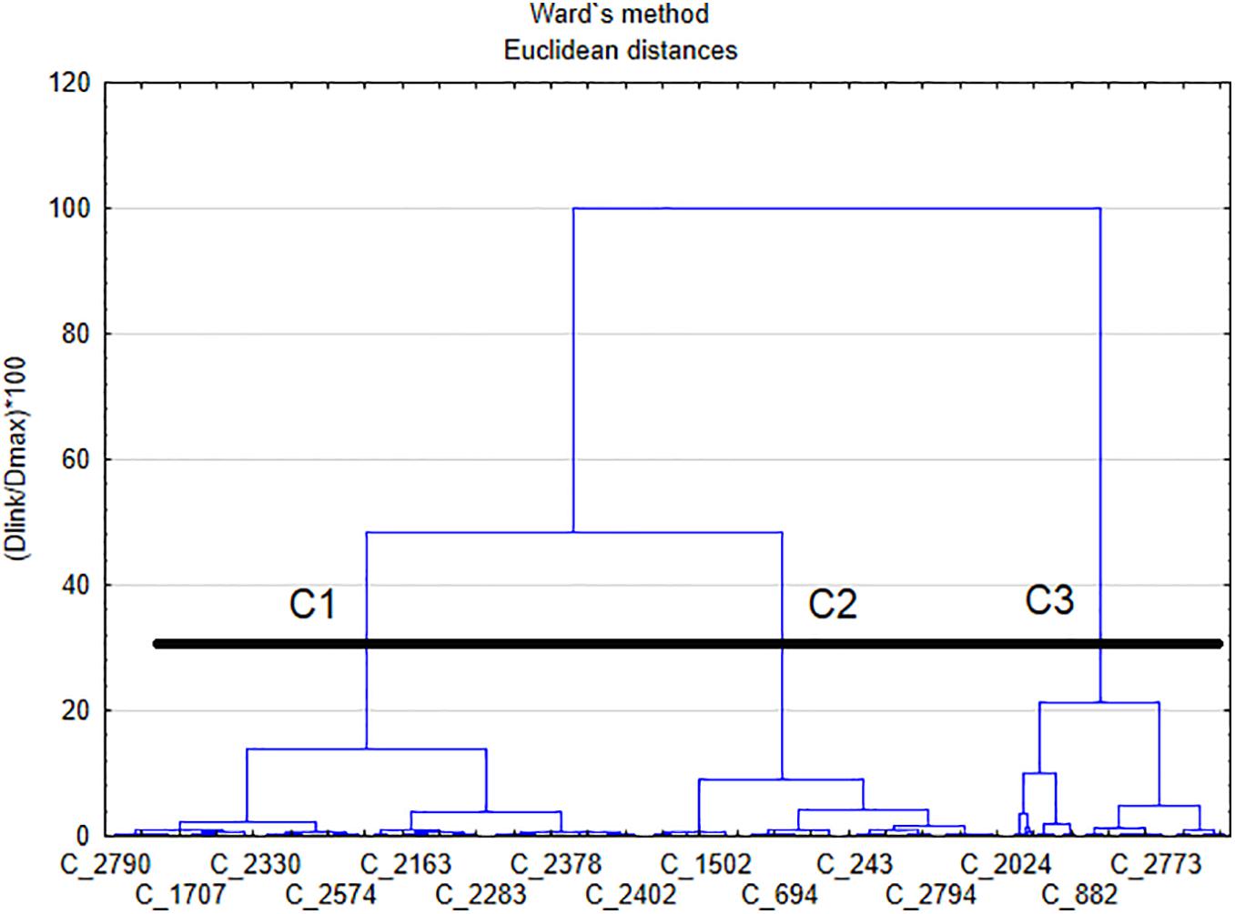
Figure 2. The dendrogram of the data points used in the work. The data are clustered into three groups: C1, C2, and C3. The x-axis represents measured air quality and meteorological data vectors, and the y-axis is the distance between points. The horizontal line represents the threshold distance between clusters we used in the work, and C_ denotes datasets.

Data Analysis

For each of the N periods, the visibility values are converted to a binary variable. It is the fundament for forecasting visibility. The binary value represented is true when visibility Vis is higher than the threshold visibility for the given period Vis_N. In parallel, we determine which M independent variables x_i has an impact on the values of Vis in a given period. The parallel M independent variables are determined with the backward stepwise algorithm. The independence of variables was checked using Spearman’s coefficient of correlation ρ. We treat two variables as dependent if the significance was at p < 0.05. The values of ρ are provided in Supplementary Table 2.

We use the logistic model to forecast the binary data. Contrary to other classification models, the result of these calculations is probability. In general, the model can be described by Equation (1) (Harrell, 2015):

$$p=\frac{\exp \left({\sum }_{i=1}^M\mathrm{\alpha }\text{⋅}\mathbf{\text{x}}+{\mathrm{\alpha }}_0\right)}{1+\exp \left({\sum }_{i=1}^M\mathrm{\alpha }\text{⋅}\mathbf{\text{x}}+{\mathrm{\alpha }}_0\right)}(1)$$

where p is the probability that Vis is greater than the specific threshold value Vis_lim, x is the vector of independent variables—air quality data or meteorological conditions, and α is the vector of the coefficients determined using the maximum likelihood estimation method (Hosmer et al., 2013). The variable is assumed to be independent if the hypothesis about the dependence of variables can be rejected at p < 0.05.

We conducted three phases of the logistic model determination: learning, testing, and validation. The data for each of these phases were selected randomly, 400 points, i.e., 3,600 points for three models and three phases.

The crucial point of the analysis was the determination of value probability p_lim for which p(Vis > Vis_lim) = p_lim. According to the value of Vis_lim, the data about visibility were divided into two classes: Vis > Vis_lim and Vis ≤ Vis_lim; we choose p_lim = 0.50 (Majewski et al., 2014). Since the preliminary analysis of the data revealed three periods with similar visibility (Figure 2), we used N = 3 models, and hence, we will determine three values of Vis_lim, three sets of independent variables (for each logistic model M₁, M₂, and M₃), and three sets of coefficients α_i.

Based on the N determined models of the forecast of Vis_{i= 1,2,…}, _N = f(x₁, x₂, …, x_j), we found empirical distributions of each of the j variables. Using these distributions, we decided to find the best fitting theoretical distribution. The choice of the distribution was done using the Kolmogorov–Smirnov (K-S) test (Massey, 1951). To get the highest compatibility of the measured and forecasted data, we analyzed the following distributions as a candidate for modeling variables (Krishnamoorthy, 2016): normal, lognormal, exponential, beta, generalized extreme value (GEV), Gumbel, Weibull, Fischer-Tippet, Johnson, Rayleigh, and Pareto with K-S test.

We used the Spearman coefficient of correlation ρ between variables and best fit theoretical distribution to build a Monte Carlo (MC) generator of synthetic time series of air quality and meteorological data. In case when variables are dependent, we used the Iman–Conover method (IC) which is a modification of the MC method (Iman and Conover, 1982). In the IC method, the variability of variables is based using marginal distributions (theoretical distributions) and the covariance is assessed by the Spearman coefficient of correlation (Chun and Tsang, 2004). Thus, the usage of this method needs to meet specific conditions (see section Conditions for the Iman–Conover method of the Supplementary Material). In our work, time series are generated using the IC method based on air quality and meteorological data except for the precipitation. We used the MC method to simulate the precipitation (P), according to the theoretical models of days with precipitation. The aim was to calculate the number of days with the precipitation n_r in the given period. The precipitation P was modeled as binary data (P = 0—no precipitation, P = 1—precipitation).

Simulation of Time Series Using Iman–Conover MC

We used our logistic models and generators to simulate time series K-times in a given period (day, week, month, etc.) of the meteorological parameters and air quality data. We used it to determine the probability that the value of Vis exceeds the limit. This procedure was repeated for each of the N models (for each model for a given variability of visibility). As a result, N cumulative distribution functions (CDFs) of the probability of the number of days with visibility higher than a specific value for every period were determined.

As a result of K = 10,000 simulations, we obtained time series with 7, 30, 365, etc. values for weekly, monthly, and yearly forecasts, respectively. We used these values to calculate p(Vis > Vis_lim1,2,3). Let’s define a function Ψ(Vis_limk,x₁,x₂,…,x_Mk) with domain for a whole forecast period in such a way:

$$\mathrm{\Psi }=\{\begin{array}{c}\hfill p({\text{Vis}}_{\text{lim}k},x_1,x_2,\mathrm{\dots },x_{M_k})>0.5\to D({\text{Vis}}_{\text{lim}})=1\hfill \\ \hfill p({\text{Vis}}_{\text{lim}k},x_1,x_2,\mathrm{\dots },x_{M_k})>0.5\to D({\text{Vis}}_{\text{lim}})=0\hfill \end{array}(2)$$

The value D is a binary parameter describing whether it is more probable that visibility is higher than Vis_lim (D = 1) or more probable that visibility is lower (D = 0). We analyzed the total number of days with visibility higher than Vis_lim for the forecast periods and the value of D_p was the number of days in the given period when the above conditions were satisfied. The expected value of D_p can be calculated using Formula (3):

$$E\left(D_{\text{p}}\right)={\displaystyle \int \int \mathrm{\dots }\int \mathrm{\Psi }(x_1,x_2,\mathrm{\dots },x_M,{\text{Vis}}_{\mathrm{lim1},2,3})\cdot f\left(x_1\right)}\mathrm{\hspace{1em}}\text{⋅}f\left(x_2\right)\mathrm{\dots }f(x_M)\text{d}{x}_1\text{d}{x}_2\mathrm{\dots }\text{d}{x}_j(3)$$

where f(x_i) is the probability density function of theoretical distribution which is the best fitting empirical distribution for variable x_i.

Since the variables in the integral above are not independent, the analytical solution is hardly feasible, and hence, we used the MC method.

Prediction Assessment

The assessment of the performance of the models is made using sensitivity (SENS) and specificity (SPEC). According to Hosmer et al. (2013) and Harrell (2015), we used also the third measure for logistic models—counting uncertainty R_z². We choose the following threshold values for further calculations: Vis_lim1 = 10 km, Vis_lim2 = 20 km, and Vis_lim3 = 30 km (Figure 2 and Supplementary Figure 2).

Finally, we used the two-sample Kolmogorov–Smirnov test to compare CDF from the logistic model and CDF from the experiment. It allowed us to evaluate numerically whether our model prediction of the number of days within the specific visibility range is in agreement with the empirical distributions of visibility.

Results and Discussion

The Logistic Regression Model

During the initial design of the model, we analyzed Vis_lim with different lowest values and different intervals between them. The Warsaw Chopin Airport, where the visibility was measured, is located at the site where visibility is good and the share of measurement with limited visibilities is low. Hence, the visibility data models with intervals lower than 10 km had poor performance. In this work, we present the performance and possibilities of the logistic regression model with three limit values. We present the modes with values Vis_lim1 = 10 km, Vis_lim2 = 20 km, and Vis_lim3 = 30 km, which have good capabilities of forecasting visibility. For example, for n_m1 = 2,517 data points, where Vis=10km (i.e., Vis_lim1 > 10km), the forecast was in agreement for 1,896 points (SENS=75.53%), while for the remaining 517 data points, 500 was in agreement (SPEC=96.65%). The value of Vis_lim is crucial for the number M of the independent variables for each model (M₁ = 7,M₂ = 6,M₃ = 5). The CDFs for three different Vis_lim divided into three periods are provided in Supplementary Figures 3–5.

Below, we present the values of coefficients α and reminding the vector of concentrations x for the logistic model described in the Data Analysis section (Equation 1). The zeros in α vectors are put for dependent variables.

$$\mathbf{\text{x}}=\left[\begin{array}{c}\hfill {\text{PM}}_{10}\hfill \\ \hfill {\text{SO}}_2\hfill \\ \hfill \text{CO}\hfill \\ \hfill {\text{NO}}_2\hfill \\ \hfill {\text{O}}_3\hfill \\ \hfill T\hfill \\ \hfill V\hfill \\ \hfill \text{Rh}\hfill \\ \hfill P\hfill \end{array}\right](4)$$

$${\mathrm{\alpha }}_I=\left[\begin{array}{c}\hfill -0.088\pm 0.007\hfill \\ \hfill -0.029=0.015\hfill \\ \hfill -0.0017\pm 0.0002\hfill \\ \hfill -0.044\pm 0.010\hfill \\ \hfill 0\hfill \\ \hfill 0.127\pm 0.014\hfill \\ \hfill 0\hfill \\ \hfill -0.257\pm 0.014\hfill \\ \hfill -0.28\pm 0.04\hfill \end{array}\right],{\mathrm{\alpha }}_{II}=\left[\begin{array}{c}\hfill -0.120\pm 0.007\hfill \\ \hfill 0\hfill \\ \hfill 0\hfill \\ \hfill -0.023\pm 0.008\hfill \\ \hfill 0.013\pm 0.005\hfill \\ \hfill 0.114\pm 0.009\hfill \\ \hfill 0\hfill \\ \hfill -0.191\pm 0.010\hfill \\ \hfill -0.55\pm 0.04\hfill \end{array}\right],$$

$${\mathrm{\alpha }}_{III}=\left[\begin{array}{c}\hfill -0.119\pm 0.007\hfill \\ \hfill 0\hfill \\ \hfill 0\hfill \\ \hfill 0\hfill \\ \hfill -0.022\pm 0.004\hfill \\ \hfill 0.10\pm 0.09\hfill \\ \hfill 0\hfill \\ \hfill -0.192\pm 0.009\hfill \\ \hfill -0.74\pm 0.08\hfill \end{array}\right](5)$$

$${\mathrm{\alpha }}_{0\text{I}}=26.0\pm 1.4,{\mathrm{\alpha }}_{0II}=18.6\pm 1.0,{\mathrm{\alpha }}_{0III}=16.2\pm 0.9(6)$$

The prediction assessment for the models we yielded is as follows: for model I, SENS = 75.53%, SPEC = 96.65%, R_z² = 93.03% based on 2,517 points in the set; for model II, SENS = 86.82%, SPEC = 89.21%, R_z² = 88.09% based on 1,616 points; and for model III, SENS = 90.21%, SPEC = 78.51%, R_z² = 86.28 % based on 1,021 points. For the chosen values of limits Vis_lim, the concentration of PM₁₀ and the values of Rh,T, and P have an impact on Vis in all the models. The solar irradiance and wind velocity are omitted in the vectors above since none of these variables was independent in any model. The increase of values of Rh, P, and PM₁₀ results in the decrease of Vis, while the increase of T results in an increase of Vis. These results are in the agreement with earlier studies (e.g., Deng et al., 2014; Majewski et al., 2015; Aman et al., 2019; Araghi et al., 2019; Won et al., 2020). The concentrations of CO and SO₂ are independent variables only in the model where Vis_lim1 = 10km, and the increase of both of them decreases visibility. NO₂ decreases the values of Vis for Vis_lim1 = 10km and Vis_lim2 = 20km.

The results of the fitting coefficients show that with the increase of Vis_lim, the positive influence of temperature decreases, while the negative influence of the concentration of PM₁₀ and the presence of precipitation increases. The increase of relative humidity decreases the probability of occurrence of the given visibility, but this influence decreases with the Vis_lim.

The sensitivity analysis of the logistic models was done using odds ratio (OR). We assumed percentage variability of marginal values of Rh₍₀₎, PM₁₀₍₀₎, and T₍₀₎ by 30%. The OR for Rh is increasing with Vis_lim from OR_Rh(Vis_lim = 10km) = 0.0058 to OR_Rh(Vis_lim = 20km) = 0.0212 to OR_Rh(Vis_lim = 30km) = 0.0217, while for T,P,andPM₁₀, the OR is decreasing with the Vis_lim (for Vis_lim = 10km, OR_PM10 = 0.49,OR_T = 1.99,OR_T = 0.75; for Vis_lim = 20km OR_PM10 = 0.39,OR_T = 1.85,OR_T = 0.58; for Vis_lim = 30km, OR_PM10 = 0.35,OR_T = 1.67,OR_T = 0.40).

The results of OR clearly show that the choice of values of Vis_lim has an impact on the sensitivity of the model and, hence, on the results of the model.

Empirical and Theoretical Distribution Fitting

Since we divided the year into N = 3 periods, our analysis of variables was also conducted in three periods. We determined empirical distributions of air quality data and meteorological data. We evaluated which of the distribution has the K-S p-value (Table 1). We provided more details in see section Distributions of the Supplementary Material.

TABLE 1

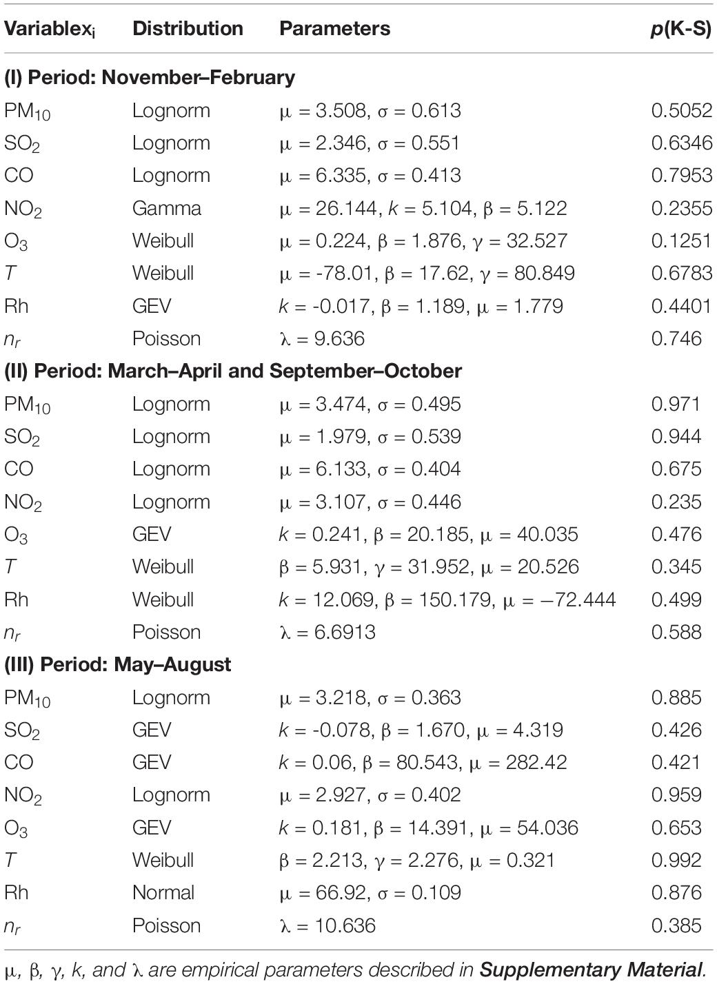
Table 1. Best fit theoretical distributions (according to the Kolmogorov–Smirnov test) for the variables.

Simulation of Visibility Occurrence

We used developed logistic models and MC generators of air quality and meteorological data to determine the number of days in month D_Vis, when visibility was in one of four ranges (defined by the chosen values of Vis_lim): (a) below 10 km, i.e., [0, 10[, (b) [10, 20[, (c) [20, 30[, and (d) [30, + ∞[. The calculations of CDFs of D_Vis were done for all three periods—three models—which were used in the work. The results are shown in Figure 3. It presents two families of CDFs: the dashed which is based on the measurement data and the continuous which is based on our model. We see that the shape of the dashed and respective continuous distributions is very similar. We verified our results using the K-S test for measurement data from the visibility monitoring station and our model. We found that for all comparisons, we could not reject the hypotheses that empirical distribution and theoretical (from the model) are the same. The probabilities (p-values of the K-S test) can be presented as the following matrix of (p_KS)_ij where i, row index, denotes period, and j describes the range of visibility: 1—[0, 10[km,[10, 20[km, 3—[20,30[km,and 4—[30, + ∞[km:

FIGURE 3

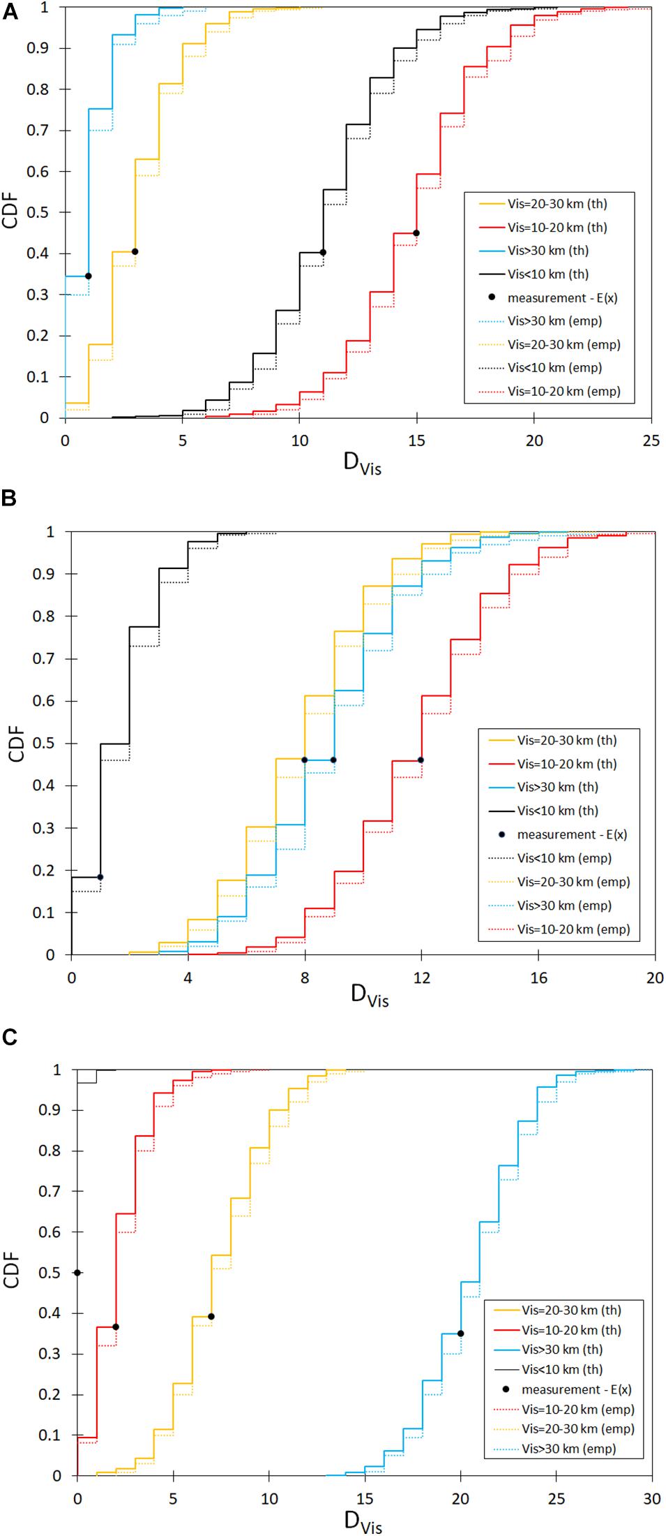
Figure 3. CDF of the number of days D_Vis in a month (30 days) with Vis in given range, “th” in the legend stands for theoretical CDF (calculated from the described model), “emp” denotes CDF from measurements, and E(x) is the expected value of D_Vis for the (A) winter period, (B) mid-period, and (C) summer period.

$$p_{\text{KS}}=\left(\begin{array}{cccc}\hfill 0.418\hfill & \hfill 0.512\hfill & \hfill 0.720\hfill & \hfill 0.792\hfill \\ \hfill 0.712\hfill & \hfill 0.512\hfill & \hfill 0.273\hfill & \hfill 0.525\hfill \\ \hfill -\hfill & \hfill 0.747\hfill & \hfill 0.563\hfill & \hfill 0.321\hfill \end{array}\right)(7)$$

Since the CDFs for Vis < 10 km in the summer period (black) in Figure 3C do not have enough degrees of freedom, we did not evaluate p_KS for this range in this period. In general, these values are high to very high, which confirms the quality of our model. We achieved that the model correctly determines the probability that the number of days with the given visibility is less or equal to a specific value.

In period I (November–February), the number of days in a month with visibility in the range [10, 20[is the highest and the median of the simulated number of days with such visibility is D_Vis = 15, while the median for the range [0, 10[is D_Vis = 11. Similarly, we found that for period II (March–April and September–October), the highest number of days in a month is for the interval [10, 20[with the median D_Vis = 12; however, the number of days in all intervals with visibility above 10 km is similar to the median number of days D_Vis = 8 for [30, + ∞[ and D_Vis = 9 for [20,30[. For period III (May–August), the median number of days in a month D_Vis = 21 is the highest for the interval [30, + ∞[.

From the application point of view, the most important is predicting the number of days with visibility in the range below 10 km since the visibility in this range is connected with aviation. Based on the curves in Figure 3, in the winter period, we see that the probability of the number of days in a month with visibility below 10 km is 𝑝 (D_Vis ≤ 21) = 1, while in the mid-period, this number of days in a month decreases to 7 and in the summer period to 2. The beginning of each curve also plays an important role in the analysis of the visibility conditions at the given site. According to Figure 3, in the winter period, we can conclude that there are always 2 days in a month with Vis = 10km since 𝑝 D_Vis = 2) = 0, while in the summer period, there are at least 13 days in a month with Vis=30km. The application of this model to another site after training allows to identify the support of the probability density function (PDF), i.e., the inverse image of open interval ]0, 1[ of values of CDF. In the case of our data, the support of PDF for VIS is as follows:

• Vis ϵ [0, 10[km is:

∘ Winter D_Vis ϵ ]2, 21[,

∘ Mid-period D_Vis ϵ ]0, 6[,

∘ Summer D_Vis ϵ ]0, 2[.

• Vis ϵ [10, 20[

∘ Winter D_Vis ϵ ]6, 24[,

∘ Mid-period D_Vis ϵ ]4, 19[,

∘ Summer D_Vis ϵ ]0, 8[.

• Vis ϵ [20, 30[km

∘ Winter D_Vis ϵ]0, 10[,

∘ Mid-period D_Vis ϵ ]2, 15[,

∘ Summer D_Vis ϵ ]1, 14[.

• Vis ϵ [30, + ∞[km

∘ Winter D_Vis ϵ ]0, 5[,

∘ Mid-period D_Vis ϵ ]3,17[,

∘ Summer D_Vis ϵ ]13,29[.

The intervals presented above are the essential description of the visibility conditions at the site we were training our model and can be applied elsewhere.

The further analysis of the CDF generated with our model gives information about the 5th percentile or the 95th percentile of the number of days in a month with specific visibility or lower. This plays an important role in the evaluation of the projects which require the assessment of limited visibility occurrence. We believe that our model can be easily applied if the sources of pollutants are similar to Warsaw and, hence, if the spatial distribution of values of the concentrations of pollutants is similar. For example, in Poland, the differences in PM₁₀ concentrations between particular regions may be high (Łowicki, 2019; GIOŚ, 2020). It is mainly caused by the high impact of local sources of emission (Rogula-Kozłowska et al., 2012, 2014; Błaszczak et al., 2020). However, the described model was developed based on the data collected in Warsaw, where air quality and sources are similar to most European cities, where the spatial distributions of concentrations of air pollutants are rather flat (Dziennik Urzędowy Województwa Mazowieckiego, 2007, 2017; Holnicki et al., 2017). It caused our proposal of visibility forecasting to be quite universal and useful for most European cities.

Data Availability Statement

Publicly available datasets were analyzed in this study. This data can be found here: Air quality data http://powietrze.gios.gov.pl/pjp/archives; Visibility data https://dane.imgw.pl/; Meteorological data are available from SGGW-WULS database on request to GM, contact: grzegorz_majewski@sggw.edu.p.

Author Contributions

GM and BS: conceptualization and methodology. JSB, TM, and AD: data curation. BS: analysis. GM and JSB: writing. JB, BS, WR-K, EA, and TM: reviewing and editing. GM and WR-K: supervision. All authors contributed to the article and approved the submitted version.

Funding

This research and APC was funded from a subsidy of the Ministry of the Interior and Administration, Poland to The Main School of Fire Service in Warsaw, Poland. The research was also a part of the project “Implementation doctorate – edition II Faculty W-7 (03DW/0001/18)” financed by the National Centre for Research and Development, Warsaw, Poland.

Conflict of Interest

The authors declare that the research was conducted in the absence of any commercial or financial relationships that could be construed as a potential conflict of interest.

Acknowledgments

We would like to thank the reviewers for the critical remarks which significantly improved the quality of the manuscript.

Supplementary Material

The Supplementary Material for this article can be found online at: https://www.frontiersin.org/articles/10.3389/fenvs.2021.623094/full#supplementary-material

References

Aman, N., Manomaiphiboon, K., Pengchai, P., Suwanathada, P., Srichawana, J., and Assareh, N. (2019). Long-term observed visibility in eastern thailand: temporal variation, association with air pollutants and meteorological factors, and trends. Atmosphere 10:122. doi: 10.3390/atmos10030122

CrossRef Full Text | Google Scholar

Araghi, A., Mousavi-Baygi, M., Adamowski, J., and Martinez, C. J. (2019). Analyzing trends of days with low atmospheric visibility in iran during 1968–2013. Environ. Monit. Assess. 191:249. doi: 10.1007/s10661-019-7381-8

PubMed Abstract | CrossRef Full Text | Google Scholar

Bennett, M. G. (1930). Physical conditions controlling visibility through the atmosphere. R. Meteorol. Soc. Q. 56, 1–30. doi: 10.1002/qj.49705623302

CrossRef Full Text | Google Scholar

Błaszczak, B., Rogula-Kozłowska, W., Mathews, B., Juda-Rezler, K., Klejnowski, K., and Rogula-Kopiec, P. (2016). Chemical compositions of PM2.5 at two non-urban sites from the polluted region in Europe. Aerosol. Air Quality Res. 16, 2333–2348. doi: 10.4209/aaqr.2015.09.0538

CrossRef Full Text | Google Scholar

Błaszczak, B., Zioła, N., Mathews, B., Klejnowski, K., and Słaby, K. (2020). The role of PM2.5 chemical composition and meteorology during high pollution periods at a suburban background station in Southern Poland. Aerosol Air Quality Res. 20, 2433–2447. doi: 10.4209/aaqr.2020.01.0013

CrossRef Full Text | Google Scholar

Chun, W. F., and Tsang, Y. P. (2004). Second-order monte carlo uncertainty/variability analysis using correlated model parameters: application to salmonid embryo survival risk assessment. Ecol. Model. 177, 393–414. doi: 10.1016/j.ecolmodel.2004.02.016

CrossRef Full Text | Google Scholar

Deng, J., Xing, Z., Zhuang, B., and Du, K. (2014). Comparative study on long-term visibility trend and its affecting factors on both sides of the taiwan strait. Atmos. Res. 143, 266–278. doi: 10.1016/j.atmosres.2014.02.018

CrossRef Full Text | Google Scholar

Deng, X., Tie, X., Wu, D., Zhou, X., Bi, X., Tan, H., et al. (2008). Long-term trend of visibility and its characterizations in the pearl river delta (PRD) region, China. Atmos. Environ. 42, 1424–1435. doi: 10.1016/j.atmosenv.2007.11.025

CrossRef Full Text | Google Scholar

Dietz, S. J., Kneringer, P., Mayr, G. J., and Zeileis, A. (2019). Forecasting low-visibility procedure states with tree-based statistical methods. Pure Appl. Geophys. 176, 2631–2644. doi: 10.1007/s00024-018-1914-x

CrossRef Full Text | Google Scholar

Ding, Y., Zhong, J., Guo, G., and Chen, F. (2020). The impact of reduced visibility caused by air pollution on construal level. Psychol. Mark. 38, 129–141.

Google Scholar

Dziennik Urzędowy Województwa Mazowieckiego (2007). ROZPORZ¥DZENIE Nr 67 WOJEWODY MAZOWIECKIEGO z Dnia 24 Grudnia 2007 r. w Sprawie Określenia Programu Ochrony Powietrza Dla Strefy Aglomeracja Warszawska. Warsaw: Masovian Voivode.

Google Scholar

Dziennik Urzędowy Województwa Mazowieckiego (2017). UCHWAŁA NR 96/17 SEJMIKU WOJEWÓDZTWA MAZOWIECKIEGO. Warsaw: Masovian Voivode.

Google Scholar

EEA (2019). Air Quality in Europe — 2019 Report. Belgium: EEA.

Google Scholar

Fajardo, O. A., Jiang, J., and Hao, J. (2013). Assessing young People’s preferences in urban visibility in Beijing. Aerosol Air Quality Res. 13, 1536–1543. doi: 10.4209/aaqr.2012.11.0307

CrossRef Full Text | Google Scholar

GIOŚ (2020). Portal Jakośæ Powietrza GIOŚ.” 2020. GIOŚ. Available online at: http://powietrze.gios.gov.pl/pjp/home (accessed February 25, 2021).

Google Scholar

Grewling, Ł, Bogawski, P., Kryza, M., Magyar, D., Šikoparija, B., Skjøth, C. A., et al. (2019). Concomitant occurrence of anthropogenic air pollutants, mineral dust and fungal spores during long-distance transport of ragweed Pollen. Environ. Pollut. 254:112948. doi: 10.1016/j.envpol.2019.07.116

PubMed Abstract | CrossRef Full Text | Google Scholar

Harrell, F. E. Jr. (2015). Regression Modeling Strategies: With Applications to Linear Models, Logistic and Ordinal Regression, and Survival Analysis. Berlin: Springer.

Google Scholar

Holnicki, P., Kałuszko, A., Nahorski, Z., Stankiewicz, K., and Trapp, W. (2017). Air Quality Modeling for Warsaw Agglomeration. Arch. Environ. Prot. 43, 48–64. doi: 10.1515/aep-2017-0005

CrossRef Full Text | Google Scholar

Hosmer, D. W. Jr., Lemeshow, S., and Sturdivant, R. X. (2013). Applied Logistic Regression, Vol. 398. Hoboken NJ: John Wiley & Sons.

Google Scholar

Hyslop, N. P. (2009). Impaired visibility: the air pollution people see. Atmos. Environ. 43, 182–195. doi: 10.1016/j.atmosenv.2008.09.067

CrossRef Full Text | Google Scholar

Iman, R. L., and Conover, W. J. (1982). A Distribution-Free Approach to Inducing Rank Correlation among Input Variables. Commun. Stati. Simulation Comput. 11, 311–334. doi: 10.1080/03610918208812265

CrossRef Full Text | Google Scholar

Kinney, P. L. (2018). Interactions of climate change, air pollution, and human health. Curr. Environ. Health Rep. 5, 179–186. doi: 10.1007/s40572-018-0188-x

PubMed Abstract | CrossRef Full Text | Google Scholar

KOBIZE (2019). Poland‘s Informative Inventory Report 2019 Submission under the UN ECE Convention on Long-Range Transboundary Air Pollution and the Directive (EU) 2016/2284. Warsaw: The National Centre for Emissions Management (KOBiZE).

Google Scholar

Krishnamoorthy, K. (2016). Handbook of Statistical Distributions with Applications. Boca Raton FL: CRC Press.

Google Scholar

Kuo, C.-Y., Cheng, F.-C., Chang, S.-Y., Lin, C.-Y., Chou, C. C., Chou, C.-H., et al. (2013). Analysis of the major factors affecting thevisibility degradation in two stations. J. Air Waste Manage. Assoc. 63, 433–441.

Google Scholar

Latha, K. M., and Badarinath, K. V. S. (2003). Black carbon aerosols over tropical urban environment—a case study. Atmos. Res. 69, 125–133. doi: 10.1016/j.atmosres.2003.09.001

CrossRef Full Text | Google Scholar

Leoni, C., Pokorná, P., Hovorka, J., Masiol, M., Topinka, J., Zhao, Y., et al. (2018). Source apportionment of aerosol particles at a european air pollution hot spot using particle number size distributions and chemical composition. Environ. Pollut. 234, 145–154. doi: 10.1016/j.envpol.2017.10.097

PubMed Abstract | CrossRef Full Text | Google Scholar

Li, X., Huang, L., Li, J., Shi, Z., Wang, Y., Zhang, H., et al. (2019). Source contributions to poor atmospheric visibility in China. Resour. Conserv. Recycling 143, 167–177.

Google Scholar

Łowicki, D. (2019). Landscape Pattern as an indicator of urban air pollution of particulate matter in Poland. Ecol. Indic. 97, 17–24. doi: 10.1016/j.ecolind.2018.09.050

CrossRef Full Text | Google Scholar

Madan, O. P., Ravi, N., and Mohanty, U. C. (2000). “A method for forecasting of visibility at hindon. Mausam 51, 47–56.

Google Scholar

Majewski, G., Czechowski, P. O., Badyda, A., and Brandyk, A. (2014). Effect of air pollution on visibility in urban conditions. warsaw case study. Environ. Prote Engi. 40, 47–64. doi: 10.5277/epe140204

CrossRef Full Text | Google Scholar

Majewski, G., Rogula-Kozłowska, W., Czechowski, P., Badyda, A., and Brandyk, A. (2015). the impact of selected parameters on visibility: first results from a long-term campaign in warsaw, Poland. Atmosphere 6, 1154–1174. doi: 10.3390/atmos6081154

CrossRef Full Text | Google Scholar

Makra, L. (2019). “Anthropogenic air pollution in ancient times,” in Toxicology in Antiquity, ed. P. Wexler [Bethesda, MD: National Library of Medicine’s (NLM) Toxicology and Environmental Health Information Program], 267–287. doi: 10.1016/B978-0-12-815339-0.00018-4

CrossRef Full Text | Google Scholar

Massey, F. J. Jr. (1951). The Kolmogorov-Smirnov Test for Goodness of Fit. Journal of the American Statistical Association 46, 68–78.

Google Scholar

PANSA (2020). METEOROLOGICAL SERVICES.” AIP POLAND. 2020. https://www.ais.pansa.pl/aip/pliki/EP_GEN_3_5_en.pdf (accessed February 25, 2021).

Google Scholar

Pastuszka, J. S., Wawroś, A., Talik, E., and Paw, K. T. U. (2003). Optical and chemical characteristics of the atmospheric aerosol in four towns in Southern Poland. Sci. Total Environ. 309, 237–251. doi: 10.1016/S0048-9697(03)00044-5

CrossRef Full Text | Google Scholar

Qu, W., Zhang, X., Wang, Y., and Fu, G. (2020). Atmospheric visibility variation over global land surface during 1973–2012: influence of meteorological factors and effect of aerosol, cloud on Abl evolution. Atmos. Pollut. Res. 11, 730–743. doi: 10.1016/j.apr.2020.01.002

CrossRef Full Text | Google Scholar

Rogula-Kozłowska, W., Klejnowski, K., Rogula-Kopiec, P., Mathews, B., and Szopa, S. (2012). A study on the seasonal mass closure of ambient fine and coarse dusts in zabrze, Poland. Bull. Environ. Contamination Toxicol. 88, 722–729. doi: 10.1007/s00128-012-0533-y

PubMed Abstract | CrossRef Full Text | Google Scholar

Rogula-Kozłowska, W., Klejnowski, K., Rogula-Kopiec, P., Ośródka, L., Krajny, E., Błaszczak, B., et al. (2014). Spatial and seasonal variability of the mass concentration and chemical composition of PM2.5 in Poland. Air Quality, Atmos. Health 7, 41–58. doi: 10.1007/s11869-013-0222-y

PubMed Abstract | CrossRef Full Text | Google Scholar

Rogula-Kozłowska, W., Kozielska, B., and Klejnowski, K. (2013). Concentration, origin and health hazard from fine particle-bound PAH at three characteristic sites in Southern Poland. Bull. Environ. Contamination and Toxicology 91, 349–355. doi: 10.1007/s00128-013-1060-1

PubMed Abstract | CrossRef Full Text | Google Scholar

Saikawa, E., Kim, H., Zhong, M., Avramov, A., Zhao, Y., Janssens-Maenhout, G., et al. (2017). Comparison of emissions inventories of anthropogenic air pollutants and greenhouse gases in China. Atmos. Chem. Phys. 17, 6393–6421. doi: 10.5194/acp-17-6393-2017

CrossRef Full Text | Google Scholar

Schedling, J. A. (1967). Anthropogenic air pollution. I. foreign substances in the air, lung affecting dust, emission and immission. Wiener Tierarztliche Monatsschrift 54, 343–348.

Google Scholar

So, R., Teakles, A., Baik, J., Vingarzan, R., and Jones, K. (2018). Development of visibility forecasting modeling framework for the lower fraser valley of British Columbia Using Canada’s regional air quality deterministic prediction system. J. Air Waste Manag.t Assoc. 68, 446–462. doi: 10.1080/10962247.2017.1416314

PubMed Abstract | CrossRef Full Text | Google Scholar

Spindler, G., Brüggemann, E., Gnauk, T., Grüner, A., Müller, K., and Herrmann, H. (2010). A Four-Year size-segregated characterization study of particles PM10, PM2.5 and PM1 Depending on Air mass origin at melpitz. Atmospheric Environment 44, 164–173. doi: 10.1016/j.atmosenv.2009.10.015

CrossRef Full Text | Google Scholar

Tsai, Y. I., Kuo, S. C., Lee, W. J., Chen, C. L., and Chen, P. T. (2007). Long-term visibility trends in one highly urbanized, one highly industrialized, and two rural areas of Taiwan. Sci. Total Environ. 382, 324–341. doi: 10.1016/j.scitotenv.2007.04.048

PubMed Abstract | CrossRef Full Text | Google Scholar

WMO (2015). Manual on the Global Observing System, Global Aspects, World Meteorological Organization WMO-No. 544, Vol. I. Geneva: WMO.

Google Scholar

Won, W. S., Oh, R., Lee, W., Kim, K. Y., Ku, S., Su, P. C., et al. (2020). Impact of Fine Particulate Matter on Visibility at Incheon International Airport, South Korea. Aerosol Air Quality Res. 20, 1048–1061. doi: 10.4209/aaqr.2019.03.0106

CrossRef Full Text | Google Scholar

Wooten, B. R., and Hammond, B. R. (2002). Macular pigment: affects visual acuity and visibility. Adv. Retinal Eye Examinat. 21, 225–240. doi: 10.1016/s1350-9462

CrossRef Full Text | Google Scholar

Zhang, R., Ashuri, B., and Deng, Y. (2017). A novel method for forecasting time series based on fuzzy logic and visibility Graph. Adv. Data Anal. Classification 11, 759–783. doi: 10.1007/s11634-017-0300-3

CrossRef Full Text | Google Scholar

Zhao, P., Zhang, X., Xu, X., and Zhao, X. (2011). Long-Term Visibility Trends and Characteristics in the Region of Beijing, Tianjin, and Hebei, China. Atmos. Res. 101, 711–718. doi: 10.1016/j.atmosres.2011.04.019

CrossRef Full Text | Google Scholar

Zhuang, X., Wang, Y., He, H., Liu, J., Wang, X., Zhu, T., et al. (2014). Haze insights and mitigation in China: an overview. J. Environ.l Sc. 26, 2–12. doi: 10.1016/S1001-0742(13)60376-9

CrossRef Full Text | Google Scholar