Detection and Sourcing of CDOM in Urban Coastal Waters With UV-Visible Imaging Spectroscopy

Introduction

Urban coastal waters are productive environments that provide important ecosystem services to humans, including the dilution of terrestrial inputs (IOCCG, 2008; Rabalais et al., 2009; McLaughlin et al., 2017), fisheries and aquaculture, and various recreational and transportation services (Halpern et al., 2012; Caron et al., 2017; Gierach et al., 2017). The rapid expansion of urban centers around the world has dramatically increased the impact of human activities on land use, runoff, hydrodynamics, atmospheric deposition, and local climate at the land-ocean interface, and these can influence the water quality of the adjacent coastal waters (McKinney, 2002; Halpern et al., 2008; Halpern et al., 2012). Increased runoff from impervious surfaces (Ackerman and Weisberg, 2003; Bay et al., 2003; Dojiri et al., 2003) and pollution point sources (e.g., wastewater effluent) can lead to elevated concentrations of nutrients, organic matter, and contaminants in urban coastal waters and negatively impact water quality in this environment. These water quality impacts have serious consequences for the services these ecosystems provide and for human health in these densely populated areas.

Chromophoric dissolved organic matter (CDOM) is a major optical water-quality indicator that can be diagnostic of runoff and point sources of pollution in urban coastal waters (IOCCG, 2015; Fichot et al., 2016; Cao et al., 2018). CDOM is ubiquitous and naturally present in coastal waters, where it is not only produced in situ by biological processes, but is also strongly influenced by terrestrial sources (e.g., soils) through runoff (Hansell and Carlson, 2014). The spectral optical properties of CDOM (absorption and fluorescence) have therefore been used in various proxies of terrestrial runoff and/or as indicators of dissolved organic matter (DOM) source and degradation state in coastal waters (Vodacek et al., 1997; Hernes and Benner, 2003; Stedmon and Markager, 2003; Boyd and Osburn, 2004; Chen et al., 2004; Helms et al., 2008; Tzortziou et al., 2008; Fichot and Benner, 2012; Murphy et al., 2013; Yamashita et al., 2013). In urban waters, wastewater effluent represents another potentially significant source of CDOM with characteristic optical properties (Goldman et al., 2012; Devlin et al., 2015), which can be leveraged and used in optical proxies indicative of CDOM-related pollution.

CDOM is optically active and therefore has the advantage of being amenable to ocean-color remote sensing (Siegel et al., 2002; Mannino et al., 2008; Swan et al., 2013; Cao et al., 2018; Werdell et al., 2018). Ocean-color remote sensing can facilitate the monitoring of several optical water quality indicators (e.g., phytoplankton, turbidity, CDOM) over large areas and could enable the detection of CDOM-related pollution in urban coastal waters (IOCCG, 2015). However, it faces major challenges in these types of waters, where a combination of difficult atmospheric corrections and optical complexity of the waters can lead to large uncertainties and errors in the derived water-quality products (Aurin and Dierssen, 2012; Werdell et al., 2018). Coastal waters are generally optically complex, (IOCCG, 2000) because they are influenced by a combination of riverine and coastal-wetland inputs, upwelling of deep water, phytoplankton blooms, and in some cases urban wastewater effluent. This optical complexity often cannot be accurately resolved using existing multispectral sensors, which have constrained spectral ranges and resolutions (Aurin and Dierssen, 2012; Dekker et al., 2018). Considering that CDOM optical properties are most prominent in the ultraviolet (UV) and blue regions, these spectral limitations are particularly restrictive for detecting CDOM and distinguishing among different CDOM sources. UV observations are beyond the spectral ranges of many current ocean color sensors, and phytoplankton can interfere with or even dominate optical variability at blue wavelengths in more phytoplankton-dominated waters (Mobley et al., 2005; Zhu et al., 2011; Fichot et al., 2016; Werdell et al., 2018).

Recent advances in imaging spectroscopy (hyperspectral imagery) with broader and finer spectral capabilities than multispectral ocean-color sensors are expected to improve retrieval accuracy for in-water constituents in complex coastal waters from remote-sensing reflectance, $R_{rs}\left(\lambda \right)$ (Mouw et al., 2015; Werdell et al., 2018). UV reflectance, in particular, is expected to facilitate the separation of chlorophyll-a and CDOM in optically complex waters. The upcoming NASA Plankton, Aerosol, Cloud, ocean Ecosystems (PACE) and Geosynchronous Littoral Imaging and Monitoring Radiometer (GLIMR) missions will provide UV-visible observations of the coastal ocean at high spectral resolution. These new spectral capabilities offer the potential to improve CDOM retrievals in optically complex coastal waters and to retrieve more specific optical properties of CDOM that are indicative of its source. However, few studies have directly assessed the utility of these new spectral capabilities for retrieving CDOM and differentiating its sources in coastal waters.

In this study, we evaluated the utility of UV-visible imaging spectroscopy for detecting CDOM accurately in urban coastal waters. We also tested the feasibility of remotely differentiating effluent-derived CDOM from other sources (e.g. terrestrial runoff). We specifically assessed the value of UV reflectance and of enhanced spectral resolution. This study took advantage of a 6-week wastewater diversion event and a related water-quality monitoring effort that took place in the urban waters of Santa Monica Bay (Southern California) in fall 2015 (City of Los Angeles, Environmental Monitoring Division, 2017; Trinh et al., 2017), and leveraged imagery from the NASA/JPL Portable Remote Imaging SpectroMeter (PRISM) airborne instrument (Mouroulis et al., 2014; Thompson et al., 2019). We used the PRISM data, as well as in-situ hyperspectral measurements of $R_{rs}\left(\lambda \right)$ and coincident laboratory measurements of CDOM spectral absorption and excitation-emission matrix (EEM) fluorescence, to compare the performance of several algorithms with varying levels of UV-visible spectral information. The data were also used to develop a fluorescence-based indicator of wastewater effluent and evaluate the amenability of this indicator to UV-visible imaging spectroscopy to detect point-source effluent. To the extent of our knowledge, this is the first attempt to use imaging spectroscopy in the UV range to facilitate water quality monitoring in coastal waters.

Study Area and Wastewater Effluent Diversion

Santa Monica Bay is a semi-enclosed coastal bay in the Southern California Bight that ranges from Malibu in the north to the Palos Verdes peninsula in the south (Figure 1). Santa Monica Bay is directly adjacent to the heavily urbanized greater Los Angeles area, which includes many densely populated coastal communities such as Santa Monica and Venice as well as the heavily trafficked Marina del Rey and Los Angeles International Airport. The bay provides valuable resources in the form of recreation, fisheries, transportation, wastewater disposal, water for industrial processes, and various other ecosystem services (Ackerman and Weisberg, 2003; Bay et al., 2003; Dojiri et al., 2003). The northern margin of Santa Monica Bay is dominated by the Santa Monica Mountains National Recreation Area, and has higher topographic relief and a sparser population (Bay et al., 2003) than the rest of the bay. Across much of the bay, water depth is less than 50 m but can reach depths greater than 500 m in submarine canyons that chisel through the bay (Figure 1).

FIGURE 1

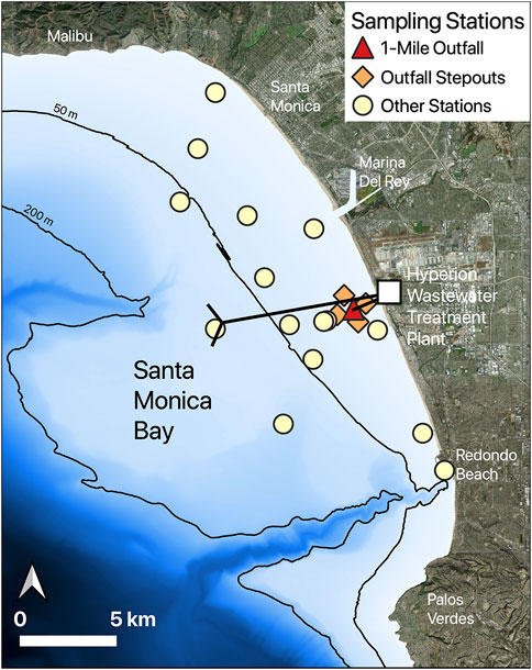
FIGURE 1. Map of Santa Monica Bay with the sampling stations including the 1-mile outfall station (D9W, red triangle), the stepout stations surrounding the outfall (orange diamonds), and the other stations (yellow circles). The 1-mile and 5-mile outfall pipes extending from the Hyperion Wastewater Treatment Plant are represented by black lines.

This urban coastal-water system consists of heterogeneous, dynamic and optically complex waters influenced by marine currents, precipitation, and point sources of nutrients (Howard et al., 2014; Howard et al., 2017) or pollution (Trinh et al., 2017). Relative to the nearby open ocean, productivity in Santa Monica Bay is high, stimulated by nutrient inputs from spring upwelling events, as well as point sources of nutrients within the bay (Bray et al., 1999). Nutrient availability and currents in the bay are also influenced by the introduction of cold waters from the California Current System, intensified by seasonal coastal upwelling (Caron et al., 2017; Trinh et al., 2017). Local currents within Santa Monica Bay are highly variable, influenced by interactions of wind and strong temperature gradients with regional currents in the Southern California Bight (Washburn et al., 2003; Caron et al., 2017; City of Los Angeles, Environmental Monitoring Division, 2017).

Santa Monica Bay receives less runoff than most river-influenced coastal margins due to the dry local climate of Southern California, with salinity in the bay typically varying over a relatively narrow range (33 ± 2 PSU) outside of terrigenous freshwater plumes (Tiefenthaler et al., 2000). Santa Monica Bay receives low riverine inputs relative to other coastal areas. Low precipitation conditions are punctuated by intermittent, although often intense, rain events (Bay et al., 2003; Dojiri et al., 2003). Runoff reaches the bay through several highly engineered, concrete-hardened urban creeks in greater Los Angeles (Ballona Creek and Santa Monica Creek) and through the more natural creek and river systems that drain the Santa Monica Mountains to the north of the bay (including Malibu Creek and Topanga Creek (Ackerman and Weisberg, 2003; Bay et al., 2003; Dojiri et al., 2003). These intermittent runoff events have been shown to substantially influence coastal water quality and biogeochemistry in the bay (City of Los Angeles, Environmental Monitoring Division, 2017).

The Hyperion Wastewater Reclamation Plant is the largest wastewater treatment facility in Los Angeles. It released approximately 230 million gallons of secondary-treated wastewater effluent into Santa Monica Bay daily in 2015 (City of Los Angeles, Environmental Monitoring Division, 2017). This effluent is treated with physically, chemically, and bacterially mediated processes to remove sediments and organo-solids. During normal operations, effluent is released through a 5-mile offshore outfall in waters that are more than 60 m deep (Lyon and Sutula, 2011; City of Los Angeles, Environmental Monitoring Division, 2017; Gierach et al., 2017; Trinh et al., 2017). In fall 2015, during scheduled maintenance lasting 6 weeks (September 21, 2015-November 2, 2015), secondary-treated effluent from Hyperion was released at an older 1-mile offshore outfall in waters less than 20 m deep (City of Los Angeles, Environmental Monitoring Division, 2017). High surface concentrations of organic matter, coliform bacteria, and algal blooms were associated with the effluent plume and impacted surface water quality. Preemptive closure of nearby beaches was therefore necessary at times during the diversion (City of Los Angeles, Environmental Monitoring Division, 2017). The water quality monitoring efforts described in this paper, including in-situ sampling, were led by the City of Los Angeles Environmental Monitoring Division (CLAEMD). Field measurements during the water quality monitoring efforts were aided by the collection of PRISM airborne imagery.

Data and Methods

In-situ Sample Collection and Measurements

Eighty-three surface water samples were collected before, during, and after the wastewater diversion (sampling from September 16-November 11, 2015) aboard the R/V La Mer and R/V Marine Surveyor along a zig-zagging pattern of stations oriented northwest-southeast in Santa Monica Bay (Figure 1 and Table 1). One station was located directly above the 1-mile Hyperion effluent outfall (Station D9W), and four more stations were positioned at “stepout” locations approximately 750 m north, south, east, and west of the outfall (Figure 1). The dispersion of the effluent from the outfall during the diversion was driven by complex and variable current patterns in Santa Monica Bay during the diversion (City of Los Angeles, Environmental Monitoring Division, 2017). As a result, some stepout stations were heavily influenced by effluent whereas others were minimally impacted. Salinity was measured at 1-m depth using an SBE 19-plus Conductivity-Temperature-Depth (CTD) rosette (Seabird Scientific®) equipped with 1.7 L Niskin bottles. Two WETLabs® WETStar single-channel fluorescence sensors were also mounted in the CTD rosette and provided simultaneous measurements of chlorophyll-a fluorescence (460 nm excitation and 695 nm emission) and DOM fluorescence (370 nm excitation and 460 nm emission). Surface water samples were collected at 1 m depth using the Niskin bottles of the CTD rosette. Samples were gravity filtered through 0.7 µm filters (GF/F glass-fiber filters) directly from the Niskin bottles into clean borosilicate EPA clear glass vials (acid washed with 10%-HCl and furnaced at 450°C for 4 h) and placed immediately at 4°C in the dark until analysis in the laboratory. Glass-fiber filters with a 0.7 µm effective pore size were used in this study as a clean filtration method that allowed samples to be rapidly filtered between sample collections. Differences between filtration through 0.7 and 0.2 µm filters are likely to be small for the relatively low particle concentrations measured in Santa Monica Bay (Laanen et al., 2011). Scattering effects from any remaining sub-micron-scale particles after 0.7 µm filtration are expected to be further mitigated by the spectral fitting routine applied during laboratory analysis for CDOM absorption (Zhu et al., 2020; described below).

TABLE 1

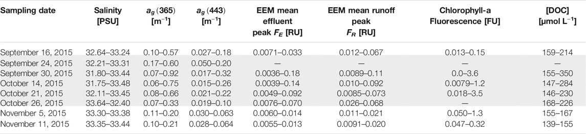
TABLE 1. Summary of in-situ variables. Ranges of observed environmental parameters are reported for each sampling day. Gray rows denote sampling conducted during the wastewater effluent diversion.

In-situ Radiometry

In-situ radiometric measurements were collected nearly simultaneously with sample collection at 45 stations using a Satlantic Inc. HyperPro free-falling optical profiling system (Seabird Scientific). The HyperPro system is composed of three, hyperspectral Satlantic Hyper Ocean Color Radiometers (HyperOCR): two HyperOCR mounted on the profiler to measure underwater downwelling irradiance $E_d\left(\lambda \right)$ and upwelling radiance $L_u\left(\lambda \right)$ and a third radiometer that measures downwelling surface irradiance above the air-water interface $E_s\left(\lambda \right)$. The HyperPro was used in two deployment methods during field sampling: tethered surface reflectance buoy mode and profiling mode. These methods are described in further detail for these data in a previous publication (Trinh et al., 2017). Briefly, in both modes, the water-leaving radiance $L_w\left(\lambda \right)$ is calculated by extrapolating below-surface upwelling radiance and downwelling irradiance measurements across the air-water interface. Water-leaving radiance is then divided by $E_s\left(\lambda \right)$, measured by the above-water reference sensor, to calculate remote sensing reflectance $R_{rs}\left(\lambda \right)=L_w\left(\lambda \right)/E_s\left(\lambda \right)$. Care was taken during both surface reflectance buoy-mode and profiler-mode deployments to keep the profiler at least 30 m away on the sunward side of the ship to minimize instrument shading. In profiler mode, observations from multiple freefall casts were combined to collect repeatable, representative $R_{rs}$ measurements. Spectral $R_{rs}\left(\lambda \right)$ measurements from the HyperPro, covered a range from 350 to 700 nm in 3–4 nm increments, but were interpolated to 1 nm spectral resolution. In-situ$R_{rs}\left(\lambda \right)$ data were smoothed using a Savitzky-Golay filter (Savitzky and Golay, 1964) with frame size of 13 nm and polynomial of order 4 (Vandermeulen et al., 2017) implemented using the sgolayfilt function in Matlab. This smoothing was selected for its preservation of spectral shape and with a window chosen to smooth spectra without eliminating narrow features (Vandermeulen et al., 2017). In-situ$R_{rs}\left(\lambda \right)$ data were used to validate PRISM $R_{rs}\left(\lambda \right)$ and to calibrate empirical algorithms. For inter-comparability with PRISM data described below, $R_{rs}\left(\lambda \right)$ analyses were limited to the 365–700 nm spectral range. $R_{rs}\left(\lambda \right)$ spectra collected at in-situ stations are shown in Supplementary Figure S1.

Chromophoric Dissolved Organic Matter Absorption Coefficient Spectra

Absorption-coefficient spectra of CDOM, $a_g\left(\lambda \right)$, were determined for the 83 surface-water samples (Figure 2) and five effluent-dilution samples (see below) using a Shimadzu UV-1830 dual-beam spectrophotometer. As described above, samples were gravity filtered using pre-combusted glass fiber filters (0.7 µm pore size) and stored at 4°C in borosilicate glass bottles prior to measurement. The absorbance (optical density) of each filtered sample was measured in 1-nm increments from 250 to 700 nm. Samples were placed in 5 cm-pathlength quartz cells, and measurements were compared to simultaneous blank measurements of pure water (Millipore Milli-Q Direct 16). Samples were allowed to equilibrate to room temperature to avoid artifacts in pure-water absorption at longer wavelengths caused by temperature differences (Sullivan et al., 2006).

FIGURE 2

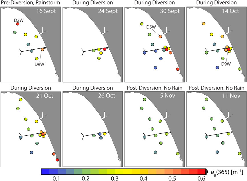
FIGURE 2. Map of in-situ a_g(365) measured during the field campaign in the fall 2015. Pre-diversion samples were measured on September 16 after a heavy precipitation event on September 15 (>6 cm of rain) and exhibited higher CDOM content at the north end of the bay. During the wastewater diversion, the highest a_g(365) were observed near the 1-mile outfall. After the end of the wastewater diversion, there was little precipitation, and a_g(365) was low at all sampling stations across Santa Monica Bay.

An exponential fit of the absorbance spectrum from 500 to 700-nm was used to compute an offset value that was subtracted from the entire absorbance spectrum (Fichot and Benner, 2011; Zhu et al., 2020). Offset-corrected spectral absorbances were converted to Napierian CDOM absorption coefficients, [m⁻¹]. This offset correction is well suited to coastal waters, because it does not assume that absorption coefficients in the 680–700 nm are negligible as is often done in procedures used to correct CDOM absorbance for open ocean waters (Johannessen et al., 2003).

Chromophoric Dissolved Organic Matter Fluorescence Excitation-Emission Matrices

Seventy-six filtered (0.7 µm) surface water samples and the five effluent-dilution samples were analyzed for excitation and emission matrix (EEM) fluorescence using a Photon Technology International PTI 814 spectrofluorometer with a 1 cm quartz cuvette (Walker et al., 2009). Excitation was performed in 5 nm increments from 240 to 450 nm, and emission was measured in 2 nm increments from 300 to 600 nm. During the measurement, the emission signal was normalized to a reference detector to remove fluctuations of the light source. The raw EEM spectra were exported to MATLAB and processed with the drEEM toolbox (Murphy et al., 2013) to correct for the inner filter effect and to apply a Raman calibration. Finally, a Raman-normalized excitation and emission spectrum of Milli-Q water (18.2 MΩ cm) was subtracted from sample EEM spectra to remove the Raman signal. EEM fluorescence was not measured on September 24 and at two stations on October 21 because of low sample volume.

Dissolved Organic Carbon Concentration

Dissolved organic carbon (DOC) was measured by high-temperature combustion using a Shimadzu TOC-V analyzer equipped with an autosampler (Fichot and Benner, 2011). Samples were gravity filtered using pre-combusted glass fiber filters (0.7 µm pore size), acidified with 2 mol L⁻¹ HCl, and stored at 4°C in borosilicate glass bottles until analysis within a few days of sampling. DOC concentration in the blanks were negligible, and accuracy and consistency of measured DOC concentrations was checked by measuring a deep seawater reference standard (University of Miami) every sixth sample.

Effluent Dilution Experiment

A sample of undiluted wastewater effluent was provided by the Hyperion Wastewater Reclamation Plant for our use in a dilution experiment. In order to simulate the effects of effluent-derived DOM on the absorption and fluorescence characteristics of the water, the effluent sample was diluted in a surface seawater sample obtained in offshore Santa Monica Bay after the diversion. Specifically, the pure effluent sample (100%) was diluted to generate seawater solutions containing 5, 1, 0.2, and 0% (no addition) of effluent by volume. Each sample was then analyzed for CDOM absorption spectra and EEM fluorescence as described above.

Algorithm Development

We developed local empirical algorithms for the remote retrieval of CDOM absorption coefficient from UV-visible $R_{rs}\left(\lambda \right)$ measurements. These algorithms were tested against two standard methods: a local empirical blue-red band ratio algorithm, and the Quasi-Analytical Algorithm version 6, updated in 2014 (QAA_V6) (Lee et al., 2007; Lee et al., 2009; Lee et al., 2014). Absorption at 365 and 443 nm were selected as representative scalar measures of CDOM to be inferred by the algorithms. The $a_g\left(365\right)$ was selected because it directly influences $R_{rs}\left(365\right)$, the shortest UV wavelength for which we have $R_{rs}\left(\lambda \right)$. The $R_{rs}\left(\lambda \right)$ in this wavelength range is expected to be less influenced by other in-water constituents. Algorithms were also developed for $a_g\left(443\right)$, to facilitate comparison with the QAA. Absorption coefficients of CDOM at 365 and 443 nm were highly correlated, and the accuracy of their retrieval by empirical algorithms was comparable, allowing for fair comparison of local empirical algorithms that utilize UV reflectance with other methods.

Empirical Algorithms for ${\mathit{a}}_{\mathit{g}}\left(\mathit{\lambda }\right)$

UV-red and blue-red band-ratio algorithms were compared to assess the utility of including UV reflectance in simple empirical algorithms to facilitate the retrieval of accurate $a_g\left(365\right)$ and $a_g\left(443\right)$ in a coastal environment where optical variability is largely driven by phytoplankton (Trinh et al., 2017). We also assessed the value of additional spectral information for the development of such empirical algorithms. Algorithms based on multiple linear regression (MLR) utilizing three bands and a full-spectrum partial least squares regression (PLSR) algorithm were compared to explore the improvements in CDOM retrieval offered by increasing spectral resolution. Specifically, to assess the utility of UV measurements and high spectral resolution data for the retrieval of $a_g\left(443\right)$, five strategies were tested:

1) univariate regression on a blue-red reflectance band ratio $R_{rs}\left(443\right)/R_{rs}\left(665\right)$;

2) univariate regression on a UV-red reflectance band ratio $R_{rs}\left(365\right)/R_{rs}\left(665\right)$;

3) visible multiple linear regression on $R_{rs}\left(412\right)$, $R_{rs}\left(443\right)$, and $R_{rs}\left(700\right)$;

4) UV-visible multiple linear regression on $R_{rs}\left(365\right)$, $R_{rs}\left(400\right)$, and $R_{rs}\left(700\right)$;

5) UV-visible partial least squares regression on full-spectrum $R_{rs}(365$$-700)$.

Empirical algorithms for deriving bio-optical properties from $R_{rs}\left(\lambda \right)$ were calibrated using in-situ data including stations where $R_{rs}\left(\lambda \right)$ was measured along with CDOM absorption (n$=$41). Empirical fits for $a_g\left(\lambda \right)$ were conducted by first taking the log-log transform of $a_g\left(443\right)$ and the $R_{rs}$ predictor variables and then performing linear regression (equivalent to fitting a power-law). For all multiple linear regression algorithms, initial wavelength selection was conducted by performing forward and backward variable selection, conducted using the MATLAB stepwiselm function to select variables based on local minimization of the Bayes Information Criterion (BIC). As stepwise variable selection is sensitive to initial selection of predictors, it was performed using reflectance observations at 5 nm intervals across the entire measured wavelength range (or from 412 to 700 for the visible-only MLR) as the initial predictor variable. The wavelengths most frequently selected by stepwise variable selection were then tested together in different combinations of wavebands, based on understanding of bio-optical signatures and chosen to reduce correlation between variables by not choosing $R_{rs}\left(\lambda \right)$ observations from wavelengths <10 nm apart. Finally, forward and backward variable selection was again conducted using the MATLAB stepwiselm function to identify a best-performing MLR model.

We also tested empirical algorithms for inferring CDOM using partial least squares regression. PLSR is a statistical technique for collapsing many highly correlated explanatory variables into a smaller number of uncorrelated predictors ranked in order of explanatory power (Mevik and Wehrens, 2007). Linear combinations of predictors are used to create components that have maximized correlation with the response variable. To predict bio-optical parameters, PLSR was implemented using the MATLAB plsregress function from the Statistics and Machine Learning Toolbox™. PLSR models were tested for both log-transformed and linear R_rs and log-transformed and linear bio-optical properties.

PLSR was tested for overfitting using a “leave-p-out” cross-validation routine with p = 4. Four data points, representing approximately 10% of the available data, was selected as an appropriate subset for validation in order to balance bias and variance in cross-validation (Arlot and Celisse, 2010). During “leave-four-out” cross-validation, PLSR coefficients were calibrated using the remaining n−4 data points, and the resulting empirical algorithm was validated using the four points that had been held out. Error statistics (root mean squared error (RMSE), mean absolute error (MAE), mean absolute percent error (MAPE), and R²) were calculated between the fitted and measured parameter of interest on the four points that were held out. This process was repeated for all possible subsets of four stations (40 choose four combinations for predicting EEM fluorescence peak ratio and 45 choose four combinations for fits on $a_g$), and averaged error statistics across all leave-four-out combinations were calculated. The averaged leave-four-out error statistics were used to select an appropriate number of PLSR components.

Full error statistics for empirical algorithm calibration are presented in Table 2. The performance of these empirical algorithms was also compared to QAA retrievals to assess the performance of locally calibrated empirical algorithms against a well-established semi-analytical approach. The same procedure was used to calibrate empirical algorithms for $a_g\left(365\right)$, but in this case no direct comparison with the QAA was possible.

TABLE 2

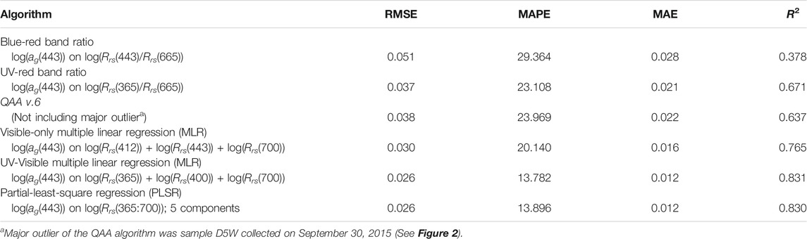
TABLE 2. Summary statistics associated with the performance comparison of the six a_g(443) algorithms (see also Figure 8). Statistics include root mean squared error (RMSE), mean average percent error (MAPE), mean absolute error (MAE), and R-squared for each algorithm.

Effluent Fluorescence Peak Ratio Empirical Algorithm Development

We also assessed the feasibility of remotely detecting CDOM source information, specifically inferring a fluorescence proxy for the degree of effluent impact. From in-situ stations where both $R_{rs}\left(\lambda \right)$ and EEM fluorescence were measured (n$=$ 40), we developed empirical algorithms for inferring the ratio between the mean intensity of an EEM fluorescence peak associated with effluent, $F_E$, (340–360 nm excitation and 426–454 nm emission), and one that was indicative of runoff-influenced CDOM, $F_R$, (255–265 nm excitation and 382–398 nm emission) from remote sensing reflectance (see Results). The effluent fluorescence ratio (EFR, mean intensity of the effluent-associated peak/mean intensity of the runoff-associated peak) was used as an optical proxy for the degree of effluent impact in a sample (see below for full definition of EFR). Unlike $F_E$, which increased with increasing CDOM regardless of source (although the increase in $F_E$ was greater for effluent-derived CDOM), EFR compared the relative intensity of fluorescence in different ranges of the spectrum. Therefore, EFR was a specific indicator of effluent, because it increased only when the amount of effluent-derived CDOM increased and was decreased by the addition of runoff-derived CDOM. Empirical algorithms utilizing MLR on $R_{rs}\left(400\right)$, $R_{rs}\left(425\right)$, and $R_{rs}\left(400\right)/R_{rs}\left(425\right)$ and a full-spectrum, $R_{rs}$(365–700), PLSR were fitted to data from 36 calibration stations with in-situ$R_{rs}$ and EEM fluorescence data.

Portable Remote Imaging SpectroMeter Imagery

PRISM imagery was collected during a flyover on October 26, 2015. The instrument, mounted on an ER-2 aircraft flying at an approximate altitude of 20 km, captured a swath from northwest to southeast along the coastline of Santa Monica Bay. Atmospheric correction was conducted using an Optimal Estimation formulation that simultaneously models surface and atmospheric reflectance contributions from statistical priors (Thompson et al., 2018). The atmospheric correction approach, including the calibration and orthorectification of the PRISM imagery were described at length in a recent manuscript (Thompson et al., 2019). The spatial resolution of the image is approximately 20 m, and includes spectral measurements made approximately every 3 nm from 350 to 1,050 nm. This high spatial resolution provides opportunities for detecting patterns in water quality at small scales, but also introduces additional challenges for interpreting data in some areas. For example, several boats are visible in maps of $R_{rs}\left(\lambda \right)$ and derived products. Reflectance measurements at wavelengths shorter than 365 nm were not available for this analysis because they were excluded during the Level-1-to-Level-2 processing of the PRISM data in order to include only spectral regions of reliable instrument calibration and atmospheric correction. PRISM swaths were trimmed to remove sensor artifacts at the edges of the swath and to remove waters with depth <10 m due to suspected influence of wave action and bottom effects in shallower waters (Supplementary Figure S2).

Statistical Analysis

Statistical analyses were conducted in R (R Core Team, 2018) and MATLAB version R2018b. Figures were produced in R using the fields package, and in MATLAB. Multiple linear regression and partial least squares regression were implemented using MATLAB version R2018b.

Results

Chromophoric Dissolved Organic Matter Variability in Santa Monica Bay

The spatial distribution of CDOM absorption in Santa Monica Bay was very variable over the course of the fall sampling, as local inputs from riverine and wastewater effluent sources were added to the bay (Figure 2). On September 16, following a major rain event before the diversion (>6 cm of rain fell on September 15 in the wettest September storm in more than 100 years), higher $a_g\left(365\right)$ values were observed nearshore and in the northern end of the bay (Figure 2), where several rivers and creeks from the Santa Monica Mountains drain to the bay. Later, during the Hyperion wastewater diversion (sampling from September 16-November 11, 2015), the highest $a_g\left(365\right)$ values (up to 0.92 m⁻¹ on September 30) were typically observed at or near the diverted 1-mile outfall (Figure 2 and Supplementary Figure S3). After the diversion, precipitation was low and $a_g\left(365\right)$ values remained low across the entire bay, with a small offshore-inshore gradient (Figure 2). This change in CDOM distribution during the sampling window illustrated several of the dominant CDOM regimes in Santa Monica Bay: 1) runoff-dominated before the diversion, 2) influenced by wastewater effluent during the diversion, and 3) low-CDOM conditions after the diversion.

The relationships between CDOM, chlorophyll-a, and salinity in this data set were complex and variable, and were consistent with variable sourcing of in-water constituents (Figure 3). Overall, these urban coastal waters exhibited general correlations between chlorophyll-a, $a_g\left(365\right),$ and salinity that were consistent with terrigenous inputs driving most of the optical variability (Bowers and Brett, 2008). However, upon close inspection, the relationships between $a_g\left(365\right)$, chlorophyll-a, and salinity clearly separated into two distinguishable trends. The first, where lower salinities were accompanied by elevated levels of chlorophyll-a and CDOM, was consistent with the influence of terrigenous inputs. The second, where lower salinities were accompanied by elevated CDOM but much more moderate levels of chlorophyll-a, corresponded to the wastewater-influenced waters of the diversion.

FIGURE 3

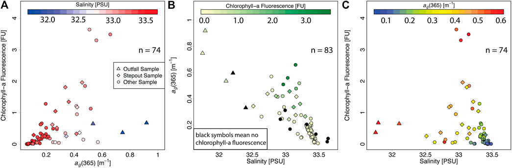
FIGURE 3. Comparison of in-situ environmental parameters measured during the field campaign: (A)a_g(365) versus chlorophyll-a fluorescence with color scale indicative of salinity, (B) salinity versus a_g(365) with color scale indicative of chlorophyll-a fluorescence, and (C) salinity versus chlorophyll-a fluorescence with color scale indicative of a_g(365). In situ chlorophyll-a fluorescence was not measured at all stations (black symbols in panel B do not have chlorophyll-a data).

Attempting to Differentiate Chromophoric Dissolved Organic Matter Sources Using Absorption

Overall, the variability of the CDOM absorption coefficient spectra adhered to expected relationships, but did not enable the identification of different CDOM sources. The absorption spectra followed the typical exponential spectral shape for CDOM (Supplementary Figure S3), and $a_g\left(\lambda \right)$ was well correlated across wavelengths. In particular, the two wavelengths explored in this study, $a_g\left(365\right)$ and $a_g\left(443\right)$, were strongly and linearly correlated with an R² = 0.99 (Figure 4A), indicating a limited range of CDOM spectral slope coefficient values in the 365–443 nm range and no obvious differences between CDOM from different sources (e.g., terrestrial runoff versus wastewater effluent). In a few cases, some $a_g\left(\lambda \right)$ spectra exhibited broad features at $\lambda$ < 360 nm that were suggestive of the presence of dissolved mycosporine-like amino acids (MAAs) exuded from phytoplankton (Morrison and Nelson, 2004; Tilstone et al., 2010). As in most coastal environments, CDOM absorption was also strongly correlated with DOC concentration (Figure 4B; (Mannino et al., 2008; Fichot and Benner, 2011)). Although this relationship remained consistent during the sampling window and enabled estimation of [DOC] from CDOM with reasonable accuracy, it did not help discriminate between different sources of CDOM.

FIGURE 4

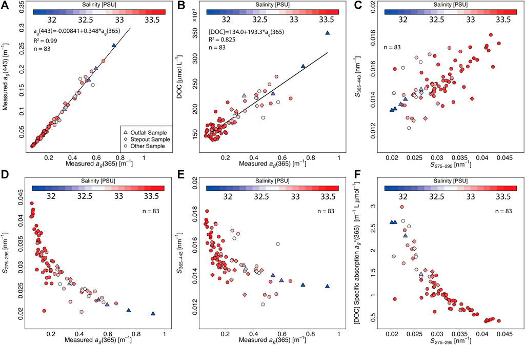
FIGURE 4. Plots of CDOM absorption characteristics: (A) relationship between absorption coefficients of CDOM at 365 and 443 nm, (B) relationship between a_g(365) and [DOC], (C) spectral slope in the UV-B (S_275–295) versus UV-A to visible (S_365–443) domain, (D) relationship between a_g(365) and S_275–295, (E) relationship between a_g(365) and S_365–443, and (F) relationship between S_{275–295 and} [DOC]-specific absorption by CDOM ($a_g^{\ast }$). Organic matter in effluent impacted samples, collected at the 1-mile outfall during the diversion, occurs in relatively high abundance, but does not differ in absorption characteristics from other CDOM sources.

Spectral slopes of CDOM absorption coefficient also did not offer opportunities to differentiate effluent-derived CDOM from other sources. Absorption spectral slopes between 275 and 295 nm ($S_{275-295}$) were correlated with UV-visible spectral slope ($S_{365-443}$), with no difference in behavior for effluent-derived CDOM (Figure 4C) from other sources. The spectral slope coefficient between 275 and 295 nm ($S_{275-295}$), a now well-established tracer of terrigenous inputs in coastal waters (Helms et al., 2008; Fichot and Benner, 2012), generally adhered to an expected power-law relationship with $a_g\left(365\right)$ and did not facilitate the discrimination of effluent-derived CDOM from other sources (Figure 4D). The UV-visible spectral slope, $S_{365-443}$, followed a similar yet less well-defined pattern, decreasing with increasing $a_g\left(365\right)$ (Figure 4E). Effluent samples did not differ in DOC-specific CDOM absorption from other CDOM sources either. The DOC-specific CDOM absorption coefficient, $a_g^{\ast }\left(365\right)=a_g\left(365\right)/\left[DOC\right]$, followed previously described relationships with $S_{275-295}$ for coastal areas (Fichot and Benner, 2012; Cao et al., 2018), and almost all samples plotted along the same general relationship (Figure 4F).

Samples collected near the effluent outfall during the diversion exhibited high $a_g\left(365\right)$, but that criterion alone was not sufficient to identify wastewater effluent, as runoff and phytoplankton blooms are also associated with elevated CDOM. Furthermore, the effluent-derived CDOM also exhibited low $S_{275-295}$ and $S_{365-443}$ values similar to those of terrigenous CDOM. The spectral shape of CDOM absorption did not differ significantly enough to facilitate the distinction of effluent-derived CDOM. Therefore, while effluent-impacted samples had relatively high CDOM, absorption alone did not offer prescriptive characteristics for separating wastewater effluent-impacted waters from riverine and autochthonous CDOM in Santa Monica Bay.

Differentiating Chromophoric Dissolved Organic Matter Sources Using Fluorescence

In contrast to CDOM absorption, EEM fluorescence proved useful for separating effluent-derived CDOM from other sources. Samples collected around the 1-mile outfall during the diversion exhibited a distinct fluorescence peak ($F_E$) often associated with wastewater effluent (sometimes described in previous literature as Peak C) (Goldman et al., 2012; Carstea et al., 2016), centered around 340–360 nm excitation and 426–454 nm emission (Figure 5). Other regions of the fluorescence EEM, such as the $F_R$ peak centered at 255–265 nm excitation and 382–398 nm emission (Figure 5), were less sensitive to effluent and more sensitive to other sources of CDOM such as runoff. These fluorescence features associated with different origins of CDOM provided an opportunity to discriminate between CDOM sources based on fluorescence.

FIGURE 5

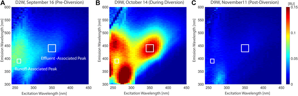
FIGURE 5. CDOM fluorescence excitation emission matrices (EEMs): (A) EEM of a pre-diversion sample with high a_g(365) associated with terrigenous runoff that fluoresces strongly at the runoff-associated peak $F_R$ (255–265 nm excitation and 382–398 nm emission), (B) EEM of an effluent-impacted sample, collected at the 1-mile outfall during the diversion, which exhibits a strong effluent-associated fluorescence peak $F_E$ (340–360 nm excitation and 426–454 nm emission) that is much less prominent in samples not influenced by effluent, (C) EEM of a low a_g(365) sample collected at the 1-mile outfall after the diversion.

Samples collected at or near the wastewater effluent outfall during the diversion fluoresced more intensely at the effluent peak (higher F_E values) than other samples with similar $a_g\left(365\right)$ values. This was evident in the observed relationship between $a_g\left(365\right)$ and F_E for all samples (Figure 6A), in which samples near the outfall clearly had enhanced F_E for the same level of $a_g\left(365\right)$. Furthermore, the samples from the effluent dilution experiment (created by diluting a sample of pure effluent provided by the Hyperion wastewater treatment plant with deep-ocean seawater) also exhibited a very similar relationship between F_E with $a_g\left(365\right)$ as the bay samples. The relationship between F_E and F_R (Figure 6B) was generally similar to the relationship between F_E and $a_g\left(365\right)$, with samples collected near the outfall exhibiting higher F_E and F_R than samples collected at other locations in Santa Monica Bay. However, samples that were solely influenced by runoff (samples collected at other locations in Santa Monica bay with relatively high a_g(365) and low salinity) exhibited much lower F_E values for the same F_R. A ratio of the two peaks captures this effluent-influenced fluorescence pattern, while limiting the influence of total CDOM content.

FIGURE 6

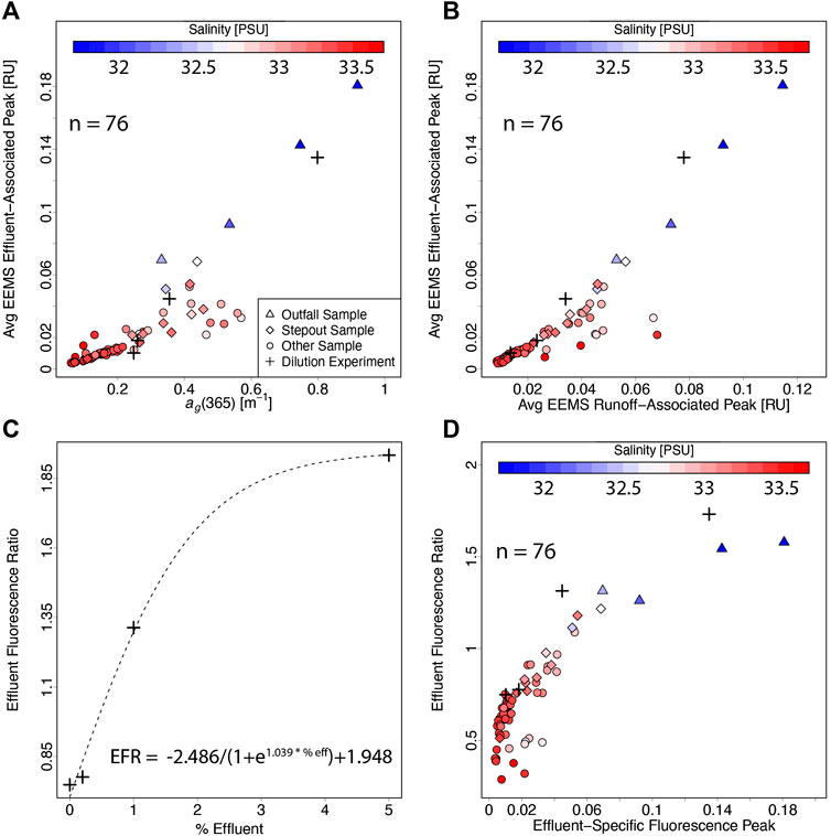
FIGURE 6. Relationships between: (A) intensity of the effluent-associated fluorescence peak $F_E$ and a_g(365), (B) intensity of effluent-associated fluorescence peak $F_E$and intensity of the runoff-associated fluorescence peak $F_R$, (C) the effluent fluorescence ratio EFR$=F_E/F_R$ and the % effluent by volume from the dilution experiment samples, and (D) the EFR and a_g(365).

The dependence of F_E and F_R on CDOM source provided an opportunity to distinguish CDOM from effluent-influenced samples. Here, we propose EFR,

$EFR=\frac{F_E}{F_R}(1)$

as an optical indicator of effluent-impacted waters, where $F_E$ is the mean fluorescence intensity in Raman Units (RU) of the effluent peak (340–360 nm excitation and 426–454 nm emission), and $F_R$ is the mean fluorescence intensity in RU for the runoff peak (255–265 nm excitation and 382–398 nm emission). EFR was selected as a specific indicator of effluent impact, because it was increased by increasing effluent-derived CDOM, but not by increasing runoff-derived CDOM. $F_E$ alone was not a specific indicator of effluent, since some samples with increased $F_E$ (>0.02 RU) were collected from both effluent-impacted and runoff-impacted waters. However, by including a ratio of $F_E/F_R$, EFR leveraged the fact that effluent-impacted CDOM had higher $F_E$ relative to other fluorescence peaks, thereby facilitating effluent detection.

The effluent dilution experiment clearly revealed the dependence of the EFR on the fraction of wastewater effluent diluted in a local seawater sample (Figure 6C). EFR values increased asymptotically with the fraction of effluent from a value of approximately 0.75 for 0% effluent to almost 2 for 5% effluent. The increased utility of EFR over $F_E$ for distinguishing samples impacted by wastewater effluent was further demonstrated by the relationship between $F_E$ and EFR for the samples collected in the bay (Figure 6D). In particular, a few runoff-impacted samples had increased $F_E$ values (∼0.2), but exhibited no such increase in EFR. Samples from the outfall during the diversion and from the effluent dilution have higher EFR than those collected at other stations, and this behavior allowed for the differentiation of effluent-derived CDOM from runoff-derived CDOM.

The spatial distribution of EFR values in Santa Monica Bay during the sampling window (Figure 7) was very consistent with the modeled dispersion of the effluent (Supplementary Figure S4). No EFR higher than 0.8 were detected before or after the diversion, and the highest EFR values detected during the diversion (>1.5) were at the wastewater outfall. Higher EFR values (>1.0) also occurred in the area surrounding the outfall (stepout stations). Samples with increased EFR generally occurred near the path of effluent plume, as inferred in particle trajectory modeling (Supplementary Figure S4) conducted by the Southern California Coastal Observatory System based high frequency radar observations of local currents in Santa Monica Bay (City of Los Angeles, Environmental Monitoring Division, 2017).

FIGURE 7

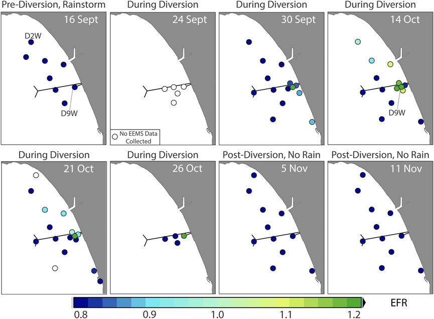
FIGURE 7. Distribution of in-situ EFR in Santa Monica Bay during the sampling window. No EEM analysis was conducted for September 24. EFR values >1.0 were only detected near the outfall during the diversion. Data from September 16 (after major rain event) show that the EFR is largely insensitive to runoff.

The effluent fluorescent peak F_E is a well-positioned fluorescence feature in CDOM because it has the potential to influence remote-sensing reflectance. This fluorescence is particularly intense, meaning it can produce a significant radiance. Furthermore, unlike most other CDOM fluorescence peaks which require excitation at wavelengths shorter than 300 nm, the F_E peak is excited by UV radiation (∼350 nm) that is naturally present in underwater solar irradiance (Fichot and Miller, 2010). It also emits broadly in the blue part of the spectrum (∼440 nm). Phytoplankton also absorb strongly in this wavelength range creating potential for fluorescence reabsorption and possibly introducing further challenges for remote detection. However, past studies (Hoge et al., 1993; Green and Blough, 1994; Lee et al., 1994), have included remote detection of CDOM fluorescence features despite interference from phytoplankton absorption, indicating that some changes in CDOM fluorescence are remotely detectable. Therefore, we expect that the sun-induced fluorescence of effluent-derived CDOM could drive detectable changes in remote-sensing reflectance, allowing for the fully remote detection of wastewater effluent based on its optical characteristics. As an optical proxy based in part on $F_E$, EFR offers utility for differentiating effluent-derived CDOM from other sources. It also offers a potential mechanism for inferring effluent influence from ocean color remote sensing. The potential applications and challenges remote EFR detection are further explored in the Discussion section in the context of the results of this work.

Algorithm Performance Comparison

We compared the performance of empirical algorithms developed for $a_g\left(443\right)$ to specifically assess the utility of: 1) $R_{rs}$ in the UV range, and 2) $R_{rs}$ at high spectral resolution (Figure 8). Our results indicated that the MLR algorithm utilizing $R_{rs}\left(365\right)$, $R_{rs}\left(400\right)$, and $R_{rs}\left(700\right)$ inferred $a_g\left(443\right)$ with the highest accuracy (full summary statistics in Table 2) between fitted and measured values (RMSE = 0.026). Despite including much more spectral information, the five-component PLSR algorithm performed similarly (RMSE = 0.026) to the MLR, suggesting that a large number of spectral bands was not necessary for retrieving CDOM accurately with empirical approaches. The MLR coefficients for all algorithms are listed in Supplementary Table S2, the PLSR component loading plots are presented in Supplementary Figure S5, and summaries of leave-four-out error for selecting number of components are presented in Supplementary Table S1. The two band ratio algorithms performed substantially worse than the empirical algorithms utilizing more predictors. The UV-red algorithm (RMSE = 0.037) performed better than the standard blue-red method (RMSE = 0.051). As expected, the UV-visible MLR (RMSE = 0.026) also outperformed the visible MLR (RMSE = 0.030). From the performance of the five empirical algorithms, we found that adding UV bands, in addition to red and blue, improved CDOM retrieval in complex coastal waters (in both the band ratio and MLR algorithms), but that increasing the number of bands (as in the PLSR algorithm) beyond three bands used in the UV-visible MLR algorithm offered minimal improvement to $a_g\left(443\right)$ retrieval accuracy.

FIGURE 8

FIGURE 8. Performance comparison of six different a_g(443) algorithms. In-situ data used for calibration (n = 41) are displayed as blue circles, and end-to-end validation points comparing measured a_g(443) to inferred a_g(443) from nearest neighbor PRISM pixels (n = 4) are displayed as orange diamonds. Most of the a_g(443) algorithms presented here, with the exception of the QAA, are empirical and were developed using coincident in-situ measurements of R_rs and a_g(443): (A) log-log fit on blue-red band ratio R_rs(443)/R_rs(665), (B) log-log fit on UV-red band ratio R_rs(365)/R_rs(665), (C) the QAA algorithm v.6, which exhibited one major outlier and is plotted without it to facilitate comparison (inset plot includes outlier), (D) log-log visible-only multiple linear regression (MLR) on R_rs(412), R_rs(443), R_rs(700); (E) log-log UV-visible MLR on R_rs(365), R_rs(400), R_rs(700), and (F) a log-log partial-least-square regression (PLSR) on the full spectrum R_rs(365–700), using the first five components. The sample collected at station D9W on October 14 was an outlier, with low inferred a_g(443) relative to measured a_g(443) for all algorithms. This sample is indicated with a dashed circle.

To compare empirical CDOM absorption retrieval to an established semi-analytical method, we included $a_g\left(443\right)$ retrieved by the QAA in our analysis. While the QAA returns spectrally-resolved water inherent optical properties (IOPs), it pools absorption by detritus ($a_d$) and $a_g$ into a combined $a_{dg}\left(\lambda \right)$ spectrum, only inferring $a_g$ independently from $a_d$ at 443 nm (Lee et al., 2014). Due to the semi-analytical, more mechanistic nature of the QAA, no calibration was conducted. The best-performing empirical algorithms for $a_g\left(443\right)$, MLR and PLSR, outperformed the QAA (RMSE = 0.038) in the complex, coastal waters of Santa Monica Bay. However, QAA retrieval of $a_g\left(443\right)$ outperformed the red-blue band ratio and had comparable accuracy to the UV-red band ratio algorithm.

Across all of the algorithms tested, the sample collected at D9W (wastewater outfall) on October 14 was an outlier, with inferred $a_g\left(443\right)$ anomalously low relative to measured $a_g\left(443\right)$ (Figure 8). This mismatch may have been caused by boat drift between radiometry and sample collection, particularly as conditions changed rapidly over steep spatial gradients around the outfall, or potential contamination of the sample. However, we did not have a definitive basis on which to exclude that data point, and therefore included it in our analyses.

Implementation of Chromophoric Dissolved Organic Matter Algorithms on Portable Remote Imaging SpectroMeter Imagery

The CDOM algorithms were implemented on the PRISM remote-sensing reflectance (Figure 9) to produce maps of CDOM at 20 m resolution in Santa Monica Bay for October 26. Mapped $R_{rs}\left(\lambda \right)$ from PRISM imagery followed reasonable distributions in Santa Monica Bay, with variability tracking different water masses. $R_{rs}\left(665\right)$ and $R_{rs}\left(555\right)$ increased in nearshore coastal areas and at the wastewater effluent outfall, highlighting areas with higher backscattering from suspended particles or phytoplankton. Distributions of $R_{rs}\left(443\right)$ and $R_{rs}\left(365\right)$ showed some similarities, with decreased reflectance in these nearshore and outfall areas, likely driven by increased CDOM and phytoplankton absorption at short wavelengths. A plume of water with decreased reflectance at $R_{rs}\left(443\right)$ and, especially, $R_{rs}\left(365\right)$ delineated a counterclockwise swirling, current-driven entrainment of material at the northern end of the bay. Overall, the observed spatial patterns of all $R_{rs}$(λ), even for $R_{rs}$(λ) in the UV domain, were very realistic and consistent with expectations for this coastal environment. To the extent of our knowledge, this represents one of the first high-resolution images of UV remote-sensing reflectance at wavelengths shorter than 380 nm collected over coastal waters.

FIGURE 9

FIGURE 9. Remote-sensing reflectance spectra, $R_{rs}\left(\lambda \right)$, measured by the airborne Portable Remote Imaging SpectroMeter (PRISM) after atmospheric correction (Thompson et al., 2019) during a flyover of Santa Monica Bay, CA on October 26, 2015: (A)$R_{rs}\left(365\right)$ map, (B)$R_{rs}\left(443\right)$ map, (C)$R_{rs}\left(555\right)$ map, (D)$R_{rs}\left(665\right)$ map, and (E) comparison of PRISM-derived $R_{rs}\left(\lambda \right)$ spectra with coincident $R_{rs}\left(\lambda \right)$ spectra measured in situ with a Satlantic HyperPro at four matchup stations: D8W, D8.5W, D9W (outfall), and D9.5W.

The spatial distributions and inferred ranges of $a_g\left(443\right)$ from the different algorithms showed expected similarities but also some important differences (Figure 10). All approaches identified a point source of high CDOM at the diverted wastewater outfall as well as plumes of CDOM swirling in Santa Monica Bay north of Marina del Rey, and smaller plumes of higher $a_g\left(443\right)$ at the north end of the bay. The location of this high $a_g\left(443\right)$ plumes in northern Santa Monica Bay is consistent with the presence of rivers and creeks draining the Santa Monica Mountains. The band ratio algorithms (Figures 10A,B) appear to overestimate $a_g\left(443\right)$ in areas with intermediate CDOM content ($0.05<a_g\left(443\right)<0.1$), relative to other strategies. Overestimation of $a_g\left(443\right)$ relative to measured data was also visible in band ratio fits of the in-situ data. Perhaps surprisingly, the maps derived from the UV-red band ratio and the blue-red band ratio exhibited similar patterns, suggesting that UV reflectance alone used in a band ratio was not sufficient to retrieve CDOM in this phytoplankton-dominated system. Similar algorithms were developed for $a_g\left(365\right)$ and these were applied to PRISM Imagery (Supplementary Table S3). Summaries of $a_g\left(365\right)$ algorithm performance and maps of $a_g\left(365\right)$ are presented in Supplementary Figures S6, S7.

FIGURE 10

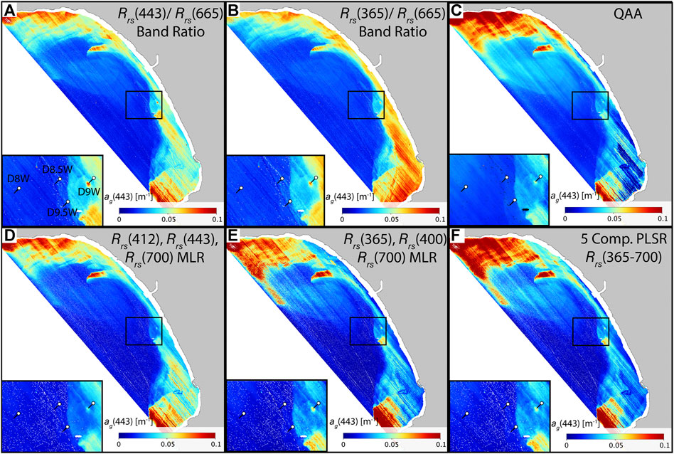
FIGURE 10. Maps of $a_g\left(443\right)$ retrieved from the PRISM $R_{rs}\left(\lambda \right)$ using the QAA and the empirical algorithms developed in this study. The $a_g\left(443\right)$ retrievals were made using the following algorithms: (A) blue-red band ratio R_rs(443)/R_rs(665), (B) UV-red band ratio R_rs(365)/R_rs(665), (C) QAA algorithm v.6, (D) visible-only multiple linear regression (MLR) on R_rs(412), R_rs(443), R_rs(700); (E) UV-visible MLR on R_rs(365), R_rs(400), R_rs(700), and (F) partial-least-square regression (PLSR) on the full spectrum R_rs(365–700) using the first five components.

We also conducted an end-to-end validation (Figure 8 and Supplementary Figure S8) for which $a_g\left(443\right)$ retrieved from PRISM $R_{rs}\left(\lambda \right)$ were compared to $a_g\left(443\right)$ measured at collocated matchup stations on October 26. However, only a very small number of data points from closely located validation stations (n = 4) were available for this validation, and these data did not provide sufficient information for reliable validation and meaningful comparison of the algorithms.

Effluent-Chromophoric Dissolved Organic Matter Detection Algorithm and Implementation on Portable Remote Imaging SpectroMeter

Algorithms for retrieving EFR were developed using a five-component PLSR on $R_{rs}$(365–700) (Figure 11). The component loading plots for the PLSR is presented in Supplementary Figure S9. The performance of this fully spectral algorithm was compared to that of a simpler algorithm based on the MLR of EFR on $R_{rs}\left(400\right)$, $R_{rs}\left(425\right)$, and $R_{rs}\left(400\right)/R_{rs}\left(425\right)$. Based on in-situ data alone, the PLSR algorithm retrieved EFR with a slightly higher accuracy (RMSE = 0.156, R² = 0.608) than the MLR algorithm (RMSE = 0.160, R² = 0.589). However, for error metrics that were comparable across parameters, (MAPE and R²), retrieval accuracies for both EFR algorithms were lower than for their corresponding $a_g\left(443\right)$ algorithms (Compare Tables 2, 3).

FIGURE 11

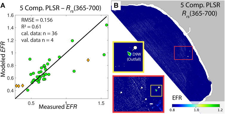
FIGURE 11. Performance of an empirical PLSR-based algorithm for Effluent Fluorescence Ratio (EFR) and its implementation on the PRISM $R_{rs}\left(\lambda \right)$ data: (A)EFR values modeled from the in-situ measured $R_{rs}\left(\lambda \right)$ using the PLSR-based algorithm, versus EFR values measured on the samples’ fluorescence EEM spectra. In-situ data used for calibration (n = 36) are displayed as green circles, and end-to-end validation points comparing measured EFR to inferred EFR from nearest neighbor PRISM pixels (n = 4) are displayed as orange diamonds. (B) Implementation of the PLSR-based algorithm on the PRISM $R_{rs}\left(\lambda \right)$ data.

TABLE 3

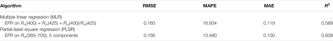
TABLE 3. Summary statistics associated with the performance comparison of the two EFR algorithms (see also Figure 11 and Supplementary Figure S10). Statistics include root mean squared error (RMSE), mean average percent error (MAPE), mean absolute error (MAE), and R-squared for each algorithm.

The EFR algorithm was applied to the PRISM imagery and generated maps of EFR at 20 m resolution across Santa Monica Bay. The range of remotely sensed EFR values matched that of the in-situ data. The map of EFR derived from the PLSR algorithm correctly detected the highest EFR at the wastewater effluent outfall (EFR between 0.85 and 1.25) and low EFR (<0.85) across the rest of Santa Monica Bay. In this respect, the PLSR algorithm appeared to successfully infer the wastewater effluent-influenced plume of DOM at the outfall, while minimizing sensitivity to CDOM from runoff and other sources. The MLR algorithm did not detect a similar maximum at the outfall (Supplementary Figure S10), and retrieved high EFR at other locations with high CDOM. Fitting and mapping of the MLR algorithm suggested that the small number of spectral $R_{rs}$ bands may not have provided sufficient information to resolve EFR independently from CDOM concentration.

Discussion

Ultraviolet Reflectance Improved Chromophoric Dissolved Organic Matter Retrievals in Urban Coastal Waters

Incorporating UV reflectance in empirical band-ratio algorithms offered only minor improvements to the accuracy of CDOM retrievals in Santa Monica Bay. A single blue-red band-ratio algorithm did not perform well in these waters and produced a spatial distribution of CDOM that closely resembled the distribution of chlorophyll-a (Trinh et al., 2017). Surprisingly, replacing the blue band (443 nm) with a UV band (365 nm), a domain where CDOM has a stronger influence, only slightly improved the accuracy of CDOM retrievals. The average percent error of $a_g\left(443\right)$ estimates decreased from approximately 30% for the red-blue ratio, to about 23% for the UV-red algorithm. This limited improvement is likely due to other in-water constituents also exerting a significant influence on UV reflectance in these waters. The dry climate of Southern California introduces less terrigenous CDOM to Santa Monica Bay compared to the more river-influenced waters typically found along the US coastline. As a result, the optical variability of the Santa Monica Bay waters tends to be strongly influenced by phytoplankton dynamics (Kahru et al., 2012; Caron et al., 2017; Trinh et al., 2017), making it more challenging to retrieve CDOM in these waters. The similarities between the mapped distribution of $a_g\left(443\right)$ inferred using the UV-red band ratio and the distribution inferred by the blue-red band ratio indicated that simply replacing a blue band by a UV one was not sufficient to remove the interference of other constituents in coastal waters strongly influenced by phytoplankton dynamics.

However, the inclusion of both UV and blue reflectance in a simple multi-band regression algorithm (MLR-based) significantly improved $a_g\left(443\right)$ retrievals. The UV-visible MLR-based algorithm combined UV, blue, and red $R_{rs}$ and performed substantially better than the simpler UV-red band ratio algorithm, producing an average percent error of <14% for $a_g\left(443\right)$. The combined use of UV and blue $R_{rs}$ in this algorithm likely facilitated the empirical differentiation between phytoplankton and CDOM. The benefit of using UV reflectance in the UV-visible MLR-based algorithm was also evident when comparing its performance to that of a similar MLR-based algorithm that used only visible bands (i.e., 412, 443, and 700 nm). The visible-only MLR-based algorithm produced slightly better results than the two band-ratio algorithms, but was outperformed by the UV-visible MLR-based algorithm, and its corresponding $a_g\left(443\right)$ map still included features influenced by phytoplankton. In contrast, the UV-visible MLR algorithm and the QAA both produced a similar $a_g\left(443\right)$ distribution that was distinct from that of phytoplankton. From the in-situ data alone, the UV-visible MLR algorithm actually outperformed the QAA. However, the QAA is not specifically optimized for the waters in Santa Monica Bay and the inclusion of UV spectral information likely offered an advantage to the UV-visible MLR-based algorithm. Overall, this analysis revealed that a simple combination of three UV, blue and red bands in a local empirical algorithm was able to retrieve $a_g\left(443\right)$ accurately and produced realistic CDOM maps in these phytoplankton-dominated waters.

The inclusion of additional spectral bands did not improve the performance of the empirical $a_g\left(443\right)$ algorithms. The PLSR algorithm leveraged all the spectral information available, but had comparable accuracy to the much simpler UV-visible MLR-based algorithm. This finding is consistent with CDOM absorption not having narrow characteristic absorption peaks like phytoplankton pigments (Rowan, 1989; Bricaud et al., 1995; Kutser et al., 2006). Instead, CDOM has a broad, featureless exponential shape, where the $a_g$variation at a single wavelength is highly predictive of that at other wavelengths. It is therefore not surprising that $a_g\left(443\right)$ was inferred with optimal accuracy from a small number of carefully chosen bands. In some cases, redundant spectral information in empirical approaches can be detrimental due to the potential of overfitting if precautions are not taken to avoid it (e.g., cross-validation as used in this study).

Although the three-band approach optimally retrieved $a_g\left(443\right)$ in Santa Monica Bay, a larger number of bands would likely prove useful or essential to retrieve CDOM accurately in more optically complex waters. The strong influence of phytoplankton in Santa Monica Bay presented some challenges for differentiating CDOM from phytoplankton. However, these waters have only moderate concentrations of in-water constituents and relatively low concentrations of non-algal particles relative to many other coastal environments, thereby avoiding challenges associated with highly absorbing and/or turbid waters (Brezonik et al., 2015; Zheng et al., 2015; Fichot et al., 2016). Accounting for the influence of non-algal particles is expected to be feasible for these applications, but might require the use of more bands. Waters in Santa Monica Bay are also mostly optically deep, so complex optical influences from bottom reflectance did not impede retrieval of water-column optical properties. Other studies have leveraged hyperspectral $R_{rs}\left(\lambda \right)$ to improve the retrieval of IOPs in waters also influenced by or bottom reflectance (Lee et al., 1994; Mobley et al., 2005; Dekker et al., 2011). Increasing the amount of spectral information, and utilizing more complex, radiative-transfer-informed approaches may be necessary to retrieve CDOM accurately in optically shallow waters.

On the Specific Detection of Effluent-Derived Chromophoric Dissolved Organic Matter

The EFR, a new fluorescence-based water quality indicator that we introduced in this study, facilitated the differentiation of effluent-derived CDOM from other sources of CDOM in coastal waters. The fact that all effluent-impacted waters in Santa Monica Bay had high CDOM, but not all high-CDOM waters were effluent-impacted presented challenges for prescriptively identifying effluent. Here, the EFR leveraged the enhanced fluorescence of effluent-impacted samples at the $F_E$ peak relative to the fluorescence at the $F_R$ peak in order to overcome this challenge. The ratio of two fluorescence peaks associated with different CDOM sources ($F_E$ being more sensitive to effluent, and $F_R$ being more sensitive to runoff) provided the means to differentiate between two sources of CDOM independently of the level of CDOM absorption observed. As a result, the EFR represents a simple but reliable potential indicator of the degree of effluent influence in these waters.

Here, we tested the feasibility of retrieving EFR empirically from remote sensing. In contrast to other CDOM fluorescence peaks in EEM spectra, the $F_E$ peak that is characteristic of the effluent CDOM (340–360 nm excitation and 426–454 nm emission) is theoretically amenable to remote sensing. The fluorescence of peak $F_E$ is stimulated in situ by UV radiation that is naturally abundant in incident solar irradiance and emits fluorescence in the blue region, thereby producing a sun-induced fluorescence signal that can influence $R_{rs}\left(\lambda \right)$. Here, the empirical algorithms developed from the in-situ data set retrieved EFR with enough accuracy (EFR error of ∼0.1) to separate samples heavily influenced by effluent. A PLSR-based algorithm retrieved EFR more accurately than the best 3-band MLR algorithm we were able to produce. When applied to PRISM data, the PLSR algorithm produced an EFR map with high values (>1.0) found only in the vicinity of the wastewater outfall. This algorithm specifically identified waters containing significant wastewater effluent, without being sensitive to CDOM from runoff or planktonic sources. In contrast, the MLR-based algorithm proved ineffective at discerning effluent-impacted EFR from the other CDOM sources, thereby suggesting the crucial importance of high spectral resolution for this purpose. While other strategies have leveraged EEMs to detect wastewater effluent (Goldman et al., 2012; Carstea et al., 2016), this is, to the extent of our knowledge, the first successful attempt at sourcing effluent-derived CDOM with remote sensing.

The presence of effluent in surface waters was only detected at relatively high concentrations of effluent. CDOM fluorescence is a relatively weak IOP, and its small influence relative to backscattering or absorption is likely responsible for the challenge of detecting effluent at low concentrations. The re-absorption of emitted fluorescence by effluent-CDOM and other absorbing constituents further decreased the influence of fluorescence signatures on ocean color. Due to the resulting small impact of fluorescence on $R_{rs}\left(\lambda \right)$, minor errors in atmospheric correction, temporal or spatial mismatch between stations and remote sensing, and measurement differences between in-situ and airborne reflectance measurements can have a disproportionate effect on retrieval accuracy. At low effluent concentrations, the optical signature of effluent-derived CDOM fluorescence is therefore expected to rapidly decrease below the detection threshold set by these practical limitations.

This feasibility study identified purely empirical relationships and did not explore the mechanistic relationship between effluent-impacted CDOM fluorescence and $R_{rs}\left(\lambda \right)$. Radiative transfer modeling of the effects of wastewater effluent fluorescence on surface $R_{rs}\left(\lambda \right)$ would help further refine the detection limits of effluent-derived CDOM. For example, the HydroLight radiative transfer numerical model (Mobley, 1989; Mobley et al., 1993; Mobley et al., 2020) already allows for the inclusion of a standard CDOM fluorescence when modeling $R_{rs}\left(\lambda \right)$, but would need to be modified to facilitate the incorporation of different types of CDOM fluorescence to help specifically assess the effects effluent-CDOM fluorescence on $R_{rs}\left(\lambda \right)$. Future avenues for this work could also include developing in-situ optical instruments leveraging the effluent-associated fluorescence peak. Prior studies have also sought to detect CDOM remotely using its fluorescence (Green and Blough, 1994; Lee et al., 1994) through stimulated fluorescence with a UV laser (Hoge et al., 1993; Vodacek et al., 1995). An active sensor providing appropriate light for fluorescence excitation could stimulate the $F_E$ peak (e.g. an 350 nm excitation and 440 nm emission) and would yield a stronger fluorescence signal in effluent impacted waters. Work also remains for generalizing this approach beyond a single effluent release scenario. A broader survey of wastewater optical characteristics across a wide range of scenarios could allow for the remote detection of source-specific optical properties different environmental settings.

Relevance to Coastal Water-Quality Monitoring With Future Ocean Color Missions

This study revealed that some improvements to CDOM-related coastal water quality monitoring can be made possible through the use of UV-visible imaging spectroscopy, an area where visible multispectral approaches have had limited success (IOCCG, 2000; Aurin and Dierssen, 2012; IOCCG, 2015; Dekker et al., 2018). The upcoming PACE and GLIMR missions will include UV-visible imaging spectrometers with comparable specifications as PRISM and are therefore expected to provide such improvements in coastal water quality monitoring. Here, the inclusion of UV reflectance (using simple-to-implement empirical algorithms) not only facilitated the accurate detection of CDOM in urban coastal waters, but also enabled its sourcing. This study also showed that high spectral resolution was essential to remotely differentiating effluent-derived CDOM. Stepping beyond the usual retrieval of $a_g$, the identification of CDOM source presents exciting opportunities for water quality monitoring in complex urban coastal waters. Improved CDOM retrievals will also help improve coastal organic-carbon budgets. The empirical relationships typically observed between $a_g\left(\lambda \right)$ and [DOC] in coastal waters (Ferrari et al., 1996; del Vecchio and Blough, 2004; Mannino et al., 2008; Fichot and Benner, 2011) will facilitate the remote quantification of DOC stores and dynamics in ocean margins (Fichot and Benner, 2014; Mannino et al., 2016; Cao et al., 2018). In turn, these will help improve carbon budgets for the coastal ocean which currently have large uncertainties (Cai, 2011; Bauer et al., 2013; Najjar et al., 2018).

The extent to which water-quality monitoring capabilities will be enhanced by UV-visible imaging spectroscopy will be contingent on our ability to apply accurate atmospheric corrections and on the availability of high-quality in‐situ validation data (IOCCG, 2012). The extended spectral range, enhanced spectral resolution, and improved signal-to-noise ratio of imaging spectrometers in upcoming missions (e.g., PACE and GLIMR) should facilitate the detection of CDOM and its subtler IOPs like effluent-CDOM fluorescence, but can only do so if accurate $R_{rs}\left(\lambda \right)$ are retrieved in the UV region. State-of-the-art atmospheric corrections and comprehensive field-validation strategies in coastal environments that include the UV region will therefore be necessary (IOCCG, 2012; Werdell et al., 2018) to achieve these improvements. Fortunately, upcoming missions like PACE will include polarimeters to better account for the contribution of various types of aerosols and are expected to facilitate atmospheric corrections and considerably improve $R_{rs}\left(\lambda \right)$ measurements in the UV and blue regions. Furthermore, ambitious field-data collection efforts are also planned in support of the PACE mission and will provide data for vicarious calibration and validation. The consistent collection of high-quality CDOM absorption and fluorescence properties (EEM) in coastal waters should be an integral part of these efforts.

Data Availability Statement

The raw data supporting the conclusion of this article will be made available by the authors, without undue reservation.

Author Contributions

JH and CF directed the study. CF led the project planning, conducted field data collection, processed in-situ radiometry, and contributed to data analysis and writing. JH led the data analysis and writing of the manuscript. KK conducted the CDOM, EEM, and DOC analyses on the samples. MG provided support for PRISM imagery collection and participated in the field data acquisition. DT conducted the atmospheric correction of the PRISM imagery. CC provided field campaign leadership and support. All authors commented and edited the manuscript.

Funding

This research was supported by a NASA Water Quality grant 80NSSC18K0344 to CF, and NASA FINESST grant 80NSSC20K1648 to graduate student JH (PI CF). Part of this research was performed at the Jet Propulsion Laboratory, California Institute of Technology, under a contract with the National Aeronautics and Space Administration (80NM0018D0004). Copyright 2020, All Rights Reserved.

Conflict of Interest

The authors declare that the research was conducted in the absence of any commercial or financial relationships that could be construed as a potential conflict of interest.

Acknowledgments

We thank the crew of the R/V La Mer and R/V Marine Surveyor, as well as the employees of the City of Los Angeles who participated in the sampling. We also thank Rebecca Trinh for her assistance in collecting radiometry data, and Jesus Mariano Duran and Frazier Peluso who helped with the analysis of CDOM samples.

Supplementary Material

The Supplementary Material for this article can be found online at: https://www.frontiersin.org/articles/10.3389/fenvs.2021.647966/full#supplementary-material

References

Ackerman, D., and Weisberg, S. B. (2003). Relationship Between Rainfall and Beach Bacterial Concentrations on Santa Monica Bay Beaches. J. Water Health 1, 85–89. doi:10.2166/wh.2003.0010

PubMed Abstract | CrossRef Full Text | Google Scholar

Arlot, S., and Celisse, A. (2010). A Survey of Cross-Validation Procedures for Model Selection. Statist. Surv. 4, 40–79. doi:10.1214/09-SS054

CrossRef Full Text | Google Scholar

Aurin, D. A., and Dierssen, H. M. (2012). Advantages and Limitations of Ocean Color Remote Sensing in CDOM-Dominated, Mineral-Rich Coastal and Estuarine Waters. Remote Sens. Environ. 125, 181–197. doi:10.1016/j.rse.2012.07.001

CrossRef Full Text | Google Scholar

Bauer, J. E., Cai, W.-J., Raymond, P. A., Bianchi, T. S., Hopkinson, C. S., and Regnier, P. A. G. (2013). The Changing Carbon Cycle of the Coastal Ocean. Nature 504, 61–70. doi:10.1038/nature12857

PubMed Abstract | CrossRef Full Text | Google Scholar

Bay, S., Jones, B. H., Schiff, K., and Washburn, L. (2003). Water Quality Impacts of Stormwater Discharges to Santa Monica Bay. Mar. Environ. Res. 56, 205–223. doi:10.1016/S0141-1136(02)00331-8

PubMed Abstract | CrossRef Full Text | Google Scholar

Bowers, D. G., and Brett, H. L. (2008). The Relationship Between CDOM and Salinity in Estuaries: An Analytical and Graphical Solution. J. Mar. Syst. 73, 1–7. doi:10.1016/j.jmarsys.2007.07.001

CrossRef Full Text | Google Scholar

Bray, N. A., Keyes, A., and Morawitz, W. M. L. (1999). The California Current System in the Southern California Bight and the Santa Barbara Channel. J. Geophys. Res. 104, 7695–7714. doi:10.1029/1998jc900038

CrossRef Full Text | Google Scholar

Brezonik, P. L., Olmanson, L. G., Finlay, J. C., and Bauer, M. E. (2015). Factors Affecting the Measurement of CDOM by Remote Sensing of Optically Complex Inland Waters. Remote Sens. Environ. 157, 199–215. doi:10.1016/j.rse.2014.04.033

CrossRef Full Text | Google Scholar

Bricaud, A., Babin, M., Morel, A., and Claustre, H. (1995). Variability in the Chlorophyll-specific Absorption Coefficients of Natural Phytoplankton: Analysis and Parameterization. J. Geophys. Res. 100, 13321–13332. doi:10.1029/95jc00463

CrossRef Full Text | Google Scholar

Boyd, T. J., and Osburn, C. L. (2004). Changes in CDOM Fluorescence From Allochthonous and Autochthonous Sources During Tidal Mixing and Bacterial Degradation in Two Coastal Estuaries. Mar. Chem. 89, 189–210. doi:10.1016/j.marchem.2004.02.012

Cai, W.-J. (2011). Estuarine and Coastal Ocean Carbon Paradox: CO2 Sinks or Sites of Terrestrial Carbon Incineration?. Annu. Rev. Mar. Sci. 3, 123–145. doi:10.1146/annurev-marine-120709-142723

PubMed Abstract | CrossRef Full Text | Google Scholar

Cao, F., Tzortziou, M., Hu, C., Mannino, A., Fichot, C. G., del Vecchio, R., et al. (2018). Remote Sensing Retrievals of Colored Dissolved Organic Matter and Dissolved Organic Carbon Dynamics in North American Estuaries and Their Margins. Remote Sens. Environ. 205, 151–165. doi:10.1016/j.rse.2017.11.014

CrossRef Full Text | Google Scholar

Caron, D. A., Gellene, A. G., Smith, J., Seubert, E. L., Campbell, V., Sukhatme, G. S., et al. (2017). Response of Phytoplankton and Bacterial Biomass During a Wastewater Effluent Diversion Into Nearshore Coastal Waters. Estuar. Coast. Shelf Sci. 186, 223–236. doi:10.1016/j.ecss.2015.09.013

CrossRef Full Text | Google Scholar

Carstea, E. M., Bridgeman, J., Baker, A., and Reynolds, D. M. (2016). Fluorescence Spectroscopy for Wastewater Monitoring: A Review. Water Res. 95, 205–219. doi:10.1016/j.watres.2016.03.021

PubMed Abstract | CrossRef Full Text | Google Scholar

Chen, R. F., Bissett, P., Coble, P., Conmy, R., Gardner, G. B., Moran, M. A., et al. (2004). Chromophoric Dissolved Organic Matter (CDOM) Source Characterization in the Louisiana Bight. Mar. Chem. 89, 257–272. doi:10.1016/j.marchem.2004.03.017

CrossRef Full Text | Google Scholar

City of Los Angeles, Environmental Monitoring Division (2017). Fall 2015 Hyperion Treatment Plant Effluent Diversion to the 1-Mile Outfall Comprehensive Monitoring Program Final Report. Los Angeles: Environmental Monitoring Division, Bureau of Sanitation, Department of Public Works, City of Los Angeles.

Dekker, A. G., Phinn, S. R., Anstee, J., Bissett, P., Brando, V. E., Casey, B., et al. (2011). Intercomparison of Shallow Water Bathymetry, Hydro-Optics, and Benthos Mapping Techniques in Australian and Caribbean Coastal Environments. Limnol. Oceanogr. Methods 9, 396–425. doi:10.4319/lom.2011.9.396

CrossRef Full Text | Google Scholar

Dekker, A. G., Pinnel, N., Gege, P., Briottet, X., Court, A., Peters, S., et al. (2018). Feasibility Study for an Aquatic Ecosystem Earth Observing System. Committee on Earth Observation Satellites. Available online: hal-02172188. (Accessed December 14, 2020).

del Vecchio, R., and Blough, N. v. (2004). Spatial and Seasonal Distribution of Chromophoric Dissolved Organic Matter and Dissolved Organic Carbon in the Middle Atlantic Bight. Mar. Chem. 89, 169–187. doi:10.1016/j.marchem.2004.02.027

CrossRef Full Text | Google Scholar

Devlin, M., Petus, C., da Silva, E., Tracey, D., Wolff, N., Waterhouse, J., et al. (2015). Water Quality and River Plume Monitoring in the Great Barrier Reef: An Overview of Methods Based on Ocean Colour Satellite Data. Remote Sens. 7, 12909–12941. doi:10.3390/rs71012909

CrossRef Full Text | Google Scholar

Dojiri, M., Yamaguchi, M., Weisberg, S. B., and Lee, H. J. (2003). Changing Anthropogenic Influence on the Santa Monica Bay Watershed. Mar. Environ. Res. 56, 1–14. doi:10.1016/S0141-1136(03)00003-5

PubMed Abstract | CrossRef Full Text | Google Scholar

Ferrari, G. M., Dowell, M. D., Grossi, S., and Targa, C. (1996). Relationship Between the Optical Properties of Chromophoric Dissolved Organic Matter and Total Concentration of Dissolved Organic Carbon in the Southern Baltic Sea Region. Mar. Chem. 55, 299–316. doi:10.1016/S0304-4203(96)00061-8

CrossRef Full Text | Google Scholar

Fichot, C. G., and Benner, R. (2011). A Novel Method to Estimate DOC Concentrations from CDOM Absorption Coefficients in Coastal Waters. Geophys. Res. Lett. 38, L03610. doi:10.1029/2010GL046152

CrossRef Full Text | Google Scholar

Fichot, C. G., and Benner, R. (2014). The Fate of Terrigenous Dissolved Organic Carbon in a River-Influenced Ocean Margin. Glob. Biogeochem. Cycles 28, 300–318. doi:10.1002/2013GB004670

CrossRef Full Text | Google Scholar

Fichot, C. G., and Benner, R. (2012). The Spectral Slope Coefficient of Chromophoric Dissolved Organic Matter (S 275-295 ) as a Tracer of Terrigenous Dissolved Organic Carbon in River-Influenced Ocean Margins. Limnol. Oceanogr. 57, 1453–1466. doi:10.4319/lo.2012.57.5.1453

CrossRef Full Text | Google Scholar

Fichot, C. G., Downing, B. D., Bergamaschi, B. A., Windham-Myers, L., Marvin-Dipasquale, M., Thompson, D. R., et al. (2016). High-Resolution Remote Sensing of Water Quality in the San Francisco Bay-Delta Estuary. Environ. Sci. Technol. 50, 573–583. doi:10.1021/acs.est.5b03518

PubMed Abstract | CrossRef Full Text | Google Scholar

Fichot, C. G., and Miller, W. L. (2010). An Approach to Quantify Depth-Resolved marine Photochemical Fluxes Using Remote Sensing: Application to Carbon Monoxide (CO) Photoproduction. Remote Sens. Environ. 114, 1363–1377. doi:10.1016/j.rse.2010.01.019

CrossRef Full Text | Google Scholar

Gierach, M. M., Holt, B., Trinh, R., Jack Pan, B., and Rains, C. (2017). Satellite Detection of Wastewater Diversion Plumes in Southern California. Estuar. Coast. Shelf Sci. 186, 171–182. doi:10.1016/j.ecss.2016.10.012

CrossRef Full Text | Google Scholar

Goldman, J. H., Rounds, S. A., and Needoba, J. A. (2012). Applications of Fluorescence Spectroscopy for Predicting Percent Wastewater in an Urban Stream. Environ. Sci. Technol. 46, 4374–4381. doi:10.1021/es2041114

PubMed Abstract | CrossRef Full Text | Google Scholar

Green, S. A., and Blough, N. V. (1994). Optical Absorption and Fluorescence Properties of Chromophoric Dissolved Organic Matter in Natural Waters. Limnol. Oceanogr. 39, 1903–1916. doi:10.4319/lo.1994.39.8.1903

Halpern, B. S., Longo, C., Hardy, D., McLeod, K. L., Samhouri, J. F., Katona, S. K., et al. (2012). An index to Assess the Health and Benefits of the Global Ocean. Nature 488, 615–620. doi:10.1038/nature11397

PubMed Abstract | CrossRef Full Text | Google Scholar

Halpern, B. S., Walbridge, S., Selkoe, K. A., Kappel, C. v., Micheli, F., D’Agrosa, C., et al. (2008). A Global Map of Human Impact on marine Ecosystems. Science 319, 948–952. doi:10.1126/science.1149345

PubMed Abstract | CrossRef Full Text | Google Scholar

Hansell, D. A., and Carlson, C. A. (2014). Biogeochemistry of Marine Dissolved Organic Matter. 2nd Edn. San Diego, CA: Elsevier.

Helms, J. R., Stubbins, A., Ritchie, J. D., Minor, E. C., Kieber, D. J., and Mopper, K. (2008). Absorption Spectral Slopes and Slope Ratios as Indicators of Molecular Weight, Source, and Photobleaching of Chromophoric Dissolved Organic Matter. Limnol. Oceanogr. 53, 955–969. doi:10.4319/lo.2008.53.3.0955

CrossRef Full Text | Google Scholar

Hernes, P. J., and Benner, R. (2003). Photochemical and Microbial Degradation of Dissolved Lignin Phenols: Implications for the Fate of Terrigenous Dissolved Organic Matter in marine Environments. J. Geophys. Res. 108, 7-1–7-9. doi:10.1029/2002jc001421

CrossRef Full Text | Google Scholar

Hoge, F. E., Vodacek, A., and Blough, N. v. (1993). Inherent Optical Properties of the Ocean: Retrieval of the Absorption Coefficient of Chromophoric Dissolved Organic Matter From Fluorescence Measurements. Limnol. Oceanogr. 38, 1394–1402. doi:10.4319/lo.1993.38.7.1394

CrossRef Full Text | Google Scholar

Howard, M. D. A., Kudela, R. M., and McLaughlin, K. (2017). New Insights Into Impacts of Anthropogenic Nutrients on Urban Ecosystem Processes on the Southern California Coastal Shelf: Introduction and Synthesis. Estuar. Coast. Shelf Sci. 186, 163–170. doi:10.1016/j.ecss.2016.06.028

CrossRef Full Text | Google Scholar

Howard, M. D. A., Sutula, M., Caron, D. A., Chao, Y., Farrara, J. D., Frenzel, H., et al. (2014). Anthropogenic Nutrient Sources Rival Natural Sources on Small Scales in the Coastal Waters of the Southern California Bight. Limnol. Oceanogr. 59, 285–297. doi:10.4319/lo.2014.59.1.0285

CrossRef Full Text | Google Scholar

IOCCG (2000). “Remote Sensing of Ocean Colour in Coastal and Other Optically-Complex Waters,” in Reports of the International Ocean-Colour Coordinating Group, No. 3. Editor S. Sathyendranath (Dartmouth, Canada: IOCCG). Available at: https://ioccg.org/wp-content/uploads/2015/10/ioccg-report-03.pdf (Accessed December 14, 2020).

Google Scholar

IOCCG (2008). “Why Ocean Colour? the Societal Benefits of Ocean-Colour Technology,” in Reports of the International Ocean-Colour Coordinating Group, No. 7. Editors T. Platt, N. Hoepffner, V. Stuart, and C. Brown (Dartmouth, Canada: IOCCG). Available at: https://ioccg.org/wp-content/uploads/2015/10/ioccg-report-07.pdf (Accessed December 14, 2020).

Google Scholar

IOCCG (2012). “Mission Requirements for Future Ocean-Colour Sensors,” in Reports of the International Ocean-Colour Coordinating Group, No. 13. Editors C. R. McClain, and G. Meister (Dartmouth, Canada: IOCCG). Available at: http://www.ioccg.org/reports/IOCCG_Report13.pdf (Accessed December 14, 2020).

Google Scholar

IOCCG (2015). “Earth Observations in Support of Global Water Quality Monitoring,” in Reports of the International Ocean-Colour Coordinating Group, No. 17. Editors A. Dekker, and C. Binding (Dartmouth, Canada: International Ocean Colour Coordinating Group). Available at: https://ioccg.org/wp-content/uploads/2018/09/ioccg_report_17-wq-rr.pdf (Accessed December 14, 2020).

Google Scholar

Johannessen, S. C., Miller, W. L., and Cullen, J. J. (2003). Calculation of UV Attenuation and Colored Dissolved Organic Matter Absorption Spectra From Measurements of Ocean Color. J. Geophys. Res. 108, 17-1–17-13. doi:10.1029/2000jc000514

CrossRef Full Text | Google Scholar

Kahru, M., di Lorenzo, E., Manzano-Sarabia, M., and Mitchell, B. G. (2012). Spatial and Temporal Statistics of Sea Surface Temperature and Chlorophyll Fronts in the California Current. J. Plankton Res. 34, 749–760. doi:10.1093/plankt/fbs010

CrossRef Full Text | Google Scholar

Kutser, T., Metsamaa, L., Strömbeck, N., and Vahtmäe, E. (2006). Monitoring Cyanobacterial Blooms by Satellite Remote Sensing. Estuar. Coast. Shelf Sci. 67, 303–312. doi:10.1016/j.ecss.2005.11.024

CrossRef Full Text | Google Scholar

Laanen, M. L., Peters, S. W. M., Dekker, A. G., and Woerd, H. J. v. d. (2011). Assessment of the Scattering by Sub-Micron Particles in Inland Waters. J. Eur. Opt. Soc. Rapid. Publ. 6, 15. doi:10.2971/jeos.2011.11046

CrossRef Full Text | Google Scholar

Lee, Z., Carder, K. L., and Arnone, R. A. (2002). Deriving Inherent Optical Properties From Water Color: A Multiband Quasi-Analytical Algorithm for Optically Deep Waters. Appl. Opt. 41, 5755. doi:10.1364/ao.41.005755

PubMed Abstract | CrossRef Full Text | Google Scholar

Lee, Z., Carder, K. L., Hawes, S. K., Steward, R. G., Peacock, T. G., and Davis, C. O. (1994). Model for the Interpretation of Hyperspectral Remote-Sensing Reflectance. Appl. Opt. 33, 5721. doi:10.1364/ao.33.005721

PubMed Abstract | CrossRef Full Text | Google Scholar

Lee, Z., Lubac, B., Werdell, J., and Arnone, R. (2009). An Update of the Quasi-Analytical Algorithm (QAA_v5). Available at: https://www.ioccg.org/groups/Software_OCA/QAA_v5.pdf (Accessed December 6, 2020).

Google Scholar

Lee, Z., Lubac, B., and Werdell, J. (2014). Update of the Quasi-Analytical Algorithm (QAA_v6). Available at: http://www.ioccg.org/groups/Software_OCA/QAA_v6_2014209.pdf (Accessed December 6, 2020).

Google Scholar

Lyon, G. S., and Sutula, M. A. (2011). “Effluent Discharges to the Southern California Bight From Large Municipal Wastewater Treatment Facilities From 2005 to 2009,” in South California Coastal Watershed Research Project Annual Report 2011, Editors Weisberg, S. B., and Miller, K.. Costa Mesa, CA, 223–236.

Google Scholar

Mannino, A., Russ, M. E., and Hooker, S. B. (2008). Algorithm Development and Validation for Satellite-Derived Distributions of DOC and CDOM in the U.S. Middle Atlantic Bight. J. Geophys. Res. 113, 1–19. doi:10.1029/2007JC004493

CrossRef Full Text | Google Scholar

Mannino, A., Signorini, S. R., Novak, M. G., Wilkin, J., Friedrichs, M. A. M., and Najjar, R. G. (2016). Dissolved Organic Carbon Fluxes in the Middle Atlantic Bight: An Integrated Approach Based on Satellite Data and Ocean Model Products. J. Geophys. Res. Biogeosci. 121, 312–336. doi:10.1002/2015JG003031

PubMed Abstract | CrossRef Full Text | Google Scholar

McKinney, M. L. (2002). Urbanization, Biodiversity, and Conservation. Bioscience 52, 583–590. doi:10.1641/0006-3568(2002)052

CrossRef Full Text | Google Scholar

McLaughlin, K., Nezlin, N. P., Howard, M. D. A., Beck, C. D. A., Kudela, R. M., Mengel, M. J., et al. (2017). Rapid Nitrification of Wastewater Ammonium Near Coastal Ocean Outfalls, Southern California, USA. Estuar. Coast. Shelf Sci. 186, 263–275. doi:10.1016/j.ecss.2016.05.013

CrossRef Full Text | Google Scholar

Mevik, B.-H., and Wehrens, R. (2007). TheplsPackage: Principal Component and Partial Least Squares Regression in R. J. Stat. Soft. 18, 1–23. doi:10.18637/jss.v018.i02

CrossRef Full Text | Google Scholar

Mobley, C. D. (1989). A Numerical Model for the Computation of Radiance Distributions in Natural Waters With Wind-Roughened Surfaces. Limnol. Oceanogr. 34, 1473–1483. doi:10.4319/lo.1989.34.8.1473

CrossRef Full Text | Google Scholar

Mobley, C. D., Boss, E., and Roesler, C. (2020). A Collaborative Web-Based Book on Optical Oceanography. Available at: https://www.oceanopticsbook.info/view/radiative-transfer-theory/level-2/hydrolight (Accessed December 21, 2020).

Google Scholar

Mobley, C. D., Gentili, B., Gordon, H. R., Jin, Z., Kattawar, G. W., Morel, A., et al. (1993). Comparison of Numerical Models for Computing Underwater Light fields. Appl. Opt. 32, 7484–7504. doi:10.1364/AO.32.007484

PubMed Abstract | CrossRef Full Text | Google Scholar

Mobley, C. D., Sundman, L. K., Davis, C. O., Bowles, J. H., Downes, T. V., Leathers, R. A., et al. (2005). Interpretation of Hyperspectral Remote-Sensing Imagery by Spectrum Matching and Look-Up Tables. Appl. Opt. 44, 3576. doi:10.1364/AO.44.003576

PubMed Abstract | CrossRef Full Text | Google Scholar

Morrison, J. R., and Nelson, N. B. (2004). Seasonal Cycle of Phytoplankton UV Absorption at the Bermuda Atlantic Time-Series Study (BATS) Site. Limnol. Oceanogr. 49, 215–224. doi:10.4319/lo.2004.49.1.0215

CrossRef Full Text | Google Scholar

Mouroulis, P., van Gorp, B., Green, R. O., Dierssen, H., Wilson, D. W., Eastwood, M., et al. (2014). Portable Remote Imaging Spectrometer Coastal Ocean Sensor: Design, Characteristics, and First Flight Results. Appl. Opt. 53, 1363. doi:10.1364/ao.53.001363

PubMed Abstract | CrossRef Full Text | Google Scholar

Mouw, C. B., Greb, S., Aurin, D., DiGiacomo, P. M., Lee, Z., Twardowski, M., et al. (2015). Aquatic Color Radiometry Remote Sensing of Coastal and Inland Waters: Challenges and Recommendations for Future Satellite Missions. Remote Sens. Environ. 160, 15–30. doi:10.1016/j.rse.2015.02.001

CrossRef Full Text | Google Scholar

Murphy, K. R., Stedmon, C. A., Graeber, D., and Bro, R. (2013). Fluorescence Spectroscopy and Multi-Way Techniques. PARAFAC. Anal. Methods 5, 6557–6566. doi:10.1039/c3ay41160e

CrossRef Full Text | Google Scholar

Najjar, R. G., Herrmann, M., Alexander, R., Boyer, E. W., Burdige, D. J., Butman, D., et al. (2018). Carbon Budget of Tidal Wetlands, Estuaries, and Shelf Waters of Eastern North America. Glob. Biogeochem. Cycles 32, 389–416. doi:10.1002/2017GB005790

CrossRef Full Text | Google Scholar

R Core Team (2018). R: A Language and Environment for Statistical Computing. Vienna, Austria: R Foundation for Statistical Computing.

Rabalais, N. N., Turner, R. E., Díaz, R. J., and Justić, D. (2009). Global Change and Eutrophication of Coastal Waters. ICES J. Mar. Sci. 66, 1528–1537. doi:10.1093/icesjms/fsp047

CrossRef Full Text | Google Scholar

Rowan, K. S. (1989). Photosynthetic Pigments of Algae. New York, NY: CUP Archive.

Savitzky, A., and Golay, M. J. E. (1964). Smoothing and Differentiation of Data by Simplified Least Squares Procedures. Anal. Chem. 36, 1627–1639. doi:10.1021/ac60214a047

CrossRef Full Text | Google Scholar

Siegel, D. A., Maritorena, S., Nelson, N. B., Hansell, D. A., and Lorenzi-Kayser, M. (2002). Global Distribution and Dynamics of Colored Dissolved and Detrital Organic Materials. J. Geophys. Res. 107, 21–1. doi:10.1029/2001jc000965

CrossRef Full Text | Google Scholar

Stedmon, C. A., and Markager, S. (2003). Behaviour of the Optical Properties of Coloured Dissolved Organic Matter Under Conservative Mixing. Estuar. Coast. Shelf Sci. 57, 973–979. doi:10.1016/S0272-7714(03)00003-9

CrossRef Full Text | Google Scholar

Sullivan, J. M., Twardowski, M. S., Zaneveld, J. R. v., Moore, C. M., Barnard, A. H., Donaghay, P. L., et al. (2006). Hyperspectral Temperature and Salt Dependencies of Absorption by Water and Heavy Water in the 400-750 nm Spectral Range. Appl. Opt. 45, 5294. doi:10.1364/AO.45.005294

PubMed Abstract | CrossRef Full Text | Google Scholar

Swan, C. M., Nelson, N. B., Siegel, D. A., and Fields, E. A. (2013). A Model for Remote Estimation of Ultraviolet Absorption by Chromophoric Dissolved Organic Matter Based on the Global Distribution of Spectral Slope. Remote Sens. Environ. 136, 277–285. doi:10.1016/j.rse.2013.05.009

CrossRef Full Text | Google Scholar

Thompson, D. R., Cawse-Nicholson, K., Erickson, Z., Fichot, C. G., Frankenberg, C., Gao, B.-C., et al. (2019). A Unified Approach to Estimate Land and Water Reflectances with Uncertainties for Coastal Imaging Spectroscopy. Remote Sens. Environ. 231, 111198. doi:10.1016/j.rse.2019.05.017

CrossRef Full Text | Google Scholar

Thompson, D. R., Natraj, V., Green, R. O., Helmlinger, M. C., Gao, B.-C., and Eastwood, M. L. (2018). Optimal Estimation for Imaging Spectrometer Atmospheric Correction. Remote Sens. Environ. 216, 355–373. doi:10.1016/j.rse.2018.07.003

CrossRef Full Text | Google Scholar

Tiefenthaler, L. L., Schiff, K. C., and Leecaster, M. K. (2000). Temporal Variability Patterns of Stormwater Concentrations in Urban Stormwater Runoff,” Southern California Coastal Water Research Project Annual Report. Westminster, CA, 52–62.

Google Scholar

Tilstone, G. H., Airs, R. L., Vicente, V. M., Widdicombe, C., Llewellyn, C., and Stramski, D. (2010). High Concentrations of Mycosporine-Like Amino Acids and Colored Dissolved Organic Matter in the Sea Surface Microlayer off the Iberian Peninsula. Limnol. Oceanogr. 55, 1835–1850. doi:10.4319/lo.2010.55.5.1835

CrossRef Full Text | Google Scholar

Trinh, R. C., Fichot, C. G., Gierach, M. M., Holt, B., Malakar, N. K., Hulley, G., et al. (2017). Application of Landsat 8 for Monitoring Impacts of Wastewater Discharge on Coastal Water Quality. Front. Mar. Sci. 4, 329. doi:10.3389/fmars.2017.00329

CrossRef Full Text | Google Scholar

Tzortziou, M., Neale, P. J., Osburn, C. L., Megonigal, J. P., Maie, N., and JaffÉ, R. (2008). Tidal Marshes as a Source of Optically and Chemically Distinctive Colored Dissolved Organic Matter in the Chesapeake Bay. Limnol. Oceanogr. 53, 148–159. doi:10.4319/lo.2008.53.1.0148

CrossRef Full Text | Google Scholar

Vandermeulen, R. A., Mannino, A., Neeley, A., Werdell, J., and Arnone, R. (2017). Determining the Optimal Spectral Sampling Frequency and Uncertainty Thresholds for Hyperspectral Remote Sensing of Ocean Color. Opt. Express 25, A785. doi:10.1364/oe.25.00a785

PubMed Abstract | CrossRef Full Text | Google Scholar

Vodacek, A., Blough, N. v., DeGrandpre, M. D., DeGrandpre, M. D., and Nelson, R. K. (1997). Seasonal Variation of CDOM and DOC in the Middle Atlantic Bight: Terrestrial Inputs and Photooxidation. Limnol. Oceanogr. 42, 674–686. doi:10.4319/lo.1997.42.4.0674

CrossRef Full Text | Google Scholar

Vodacek, A., Hogel, F. E., Swift, R. N., Yungel, J. K., Peltzer, E. T., and Blough, N. V. (1995). The Use of In Situ and Airborne Fluorescence Measurements to Determine UV Absorption Coefficients and DOC Concentrations in Surface Waters. Limnol. Oceanogr. 40, 411–415. doi:10.4319/lo.1995.40.2.0411

CrossRef Full Text | Google Scholar

Walker, S. A., Amon, R. M. W., Stedmon, C., Duan, S., and Louchouarn, P. (2009). The Use of PARAFAC Modeling to Trace Terrestrial Dissolved Organic Matter and Fingerprint Water Masses in Coastal Canadian Arctic Surface Waters. J. Geophys. Res. 114, 1–12. doi:10.1029/2009JG000990

CrossRef Full Text | Google Scholar

Washburn, L., McClure, K. A., Jones, B. H., and Bay, S. M. (2003). Spatial Scales and Evolution of Stormwater Plumes in Santa Monica Bay. Mar. Environ. Res. 56, 103–125. doi:10.1016/S0141-1136(02)00327-6

PubMed Abstract | CrossRef Full Text | Google Scholar

Werdell, P. J., McKinna, L. I. W., Boss, E., Ackleson, S. G., Craig, S. E., Gregg, W. W., et al. (2018). An Overview of Approaches and Challenges for Retrieving marine Inherent Optical Properties from Ocean Color Remote Sensing. Prog. Oceanogr. 160, 186–212. doi:10.1016/j.pocean.2018.01.001

PubMed Abstract | CrossRef Full Text | Google Scholar

Yamashita, Y., Boyer, J. N., and Jaffé, R. (2013). Evaluating the Distribution of Terrestrial Dissolved Organic Matter in a Complex Coastal Ecosystem Using Fluorescence Spectroscopy. Cont. Shelf Res. 66, 136–144. doi:10.1016/j.csr.2013.06.010

CrossRef Full Text | Google Scholar

Zheng, G., Stramski, D., and Digiacomo, P. M. (2015). A Model for Partitioning the Light Absorption Coefficient of Natural Waters Into Phytoplankton, Nonalgal Particulate, and Colored Dissolved Organic Components: A Case Study for the Chesapeake Bay. J. Geophys. Res. Oceans 120, 2601–2621. doi:10.1002/2014JC010604

CrossRef Full Text | Google Scholar

Zhu, W., Yu, Q., Tian, Y. Q., Chen, R. F., and Gardner, G. B. (2011). Estimation of Chromophoric Dissolved Organic Matter in the Mississippi and Atchafalaya River Plume Regions Using Above-Surface Hyperspectral Remote Sensing. J. Geophys. Res. 116, 1–22. doi:10.1029/2010JC006523

CrossRef Full Text | Google Scholar

Zhu, X., Miller, W. L., and Fichot, C. G. (2020). Simple Method to Determine the Apparent Quantum Yield Matrix of CDOM Photobleaching in Natural Waters. Environ. Sci. Technol. 54, 14096–14106. doi:10.1021/acs.est.0c03605

PubMed Abstract | CrossRef Full Text | Google Scholar