Experimental Design and Interpretation of Terrestrial Ecosystem Studies Using 15N Tracers: Practical and Statistical Considerations

Introduction

System ecology and biogeochemistry focus on the dynamics of substances or energy in ecosystems. To monitor the flows of elements through the different pools of an ecosystem, tracers can be an extremely useful tool (Fry, 2006). Nitrogen (N) consists mainly of the stable isotope ¹⁴N, with the heavier stable isotope ¹⁵N making up a small proportion (0.3663% of the atoms in atmospheric N₂). N compounds with a non-natural ¹⁵N content can thus be used as a tracer. As such, they make it possible to study the dynamics of N in ecosystems, especially the double role of this element as an essential but also potentially harmful element. N is indeed an essential component of all organisms and plays a role in practically all biological processes. On the other hand, since the beginning of the 20th century, humans have enormously increased its availability in the environment by converting N₂ into biologically reactive forms of N. This occurs partly on purpose, through the production of N fertilizers and partly as oxidation byproducts in combustion processes. In many cases this increase has led to eutrophication, acidification and a decrease in the biodiversity of ecosystems (Erisman et al., 2011).

According to Hauck and Bremner (1976), the use of ¹⁵N in biological research started around 1940, not long after it became possible to produce substances enriched in this isotope. The first applications were in investigations of plant N uptake from decomposing plant material or from fertilizers. In the following decades, there were hundreds of publications on agricultural research involving ¹⁵N. Around 1970, N isotope ratios could only be determined with a precision that was in the same order of magnitude as variations observed in different natural sources (Hauck et al., 1972). At that time, ¹⁵N started to be used in large-scale field research, still mostly in agricultural systems [Hauck and Bremner, 1976; Nadelhoffer and Fry, 1994; see also a synthesis by; Gardner and Drinkwater (2009)]. One of the oldest experiments in a forest was conducted in Sweden in the 1960s (Nömmik, 1966; Björkman et al., 1967). A tracer experiment in an alpine grassland in Austria was started in the 1970s and was resampled 27 years later (Gerzabek et al., 2004). According to Nadelhoffer and Fry (1994), large-scale ¹⁵N tracer experiments were still a relatively new development in the 1990s. At that time, the analytical precision had improved and became sufficient to even measure variations in ¹⁵N natural abundance. For ¹⁵N tracer studies, this meant that measurements had become possible even in large ecosystem pools in which the tracer would be strongly diluted. Currently, routine measurements by isotope-ratio mass spectrometry (IRMS) have an accuracy better than one thousandth of the natural abundance, which corresponds to approximately 1 out of 300,000 N atoms in a sample. As an example, it is possible to apply just 1 g or even less of a highly enriched nitrate salt (e.g. KNO₃ with 99% ¹⁵N) to the soil under a large conifer tree (500 kg biomass), and to quantitatively measure how much of this tracer is recovered in the foliage one year later. And this can be achieved by analyzing a sample weighing less than a single needle of the tree.

Because of improvements in the techniques and a reduction of costs, field studies using ¹⁵N as a tracer have increased considerably in popularity. Based on knowledge gained from our own experiments, during counseling activities and through discussions with other researchers (in particular Templer et al., 2012), we want here to summarize methodological aspects of such studies. We will focus on terrestrial ecosystems, mainly on unfertilized ones. We will discuss the setup of experiments, the application of the tracer, the sampling of the various parts of the ecosystem, and the calculation of the tracer recoveries. Finally, we will discuss some examples of how results can be interpreted. Of course, each experiment has its own questions and hypotheses, which affect the choice of methods, but the overall aim of tracer field experiments is to determine the fate of the labeled compounds and to infer about process rates. In this respect, a number of general principles deserve consideration. The goal of the present contribution is, thus, to help researchers in planning, conducting and interpreting ¹⁵N tracer field experiments.

Experimental Design

Field experiments with labeled N have the advantage that they can be run for a long time, even years, without disturbing the natural conditions of the system. Due to the complexity of the N cycle in an ecosystem, especially in the soil, field tracer studies usually do not have the aim of quantifying a specific process like N mineralization or nitrification. Using ¹⁵N to measure such processes generally requires bringing soil samples to the laboratory and mixing the tracer with the soil, thus disturbing its natural structure. Relatively short incubation periods are then applied, in the order of magnitude of one day (e.g. Wessel and Tietema, 1992; Schleppi et al., 2019). Instead, the aim of field studies is to describe the overall fate of the applied tracer. In this approach, the interpretation of recovery rates is relatively straight forward, especially if the tracer is added to a preexisting N flux into or within the ecosystem. The best examples are ¹⁵N added to fertilizer, applied as simulated atmospheric deposition, or applied as labeled plant litter. In many cases, however, single (net or gross) process rates are difficult to estimate from such experiments because pathways of N within the system are multiple and partly bidirectional. Two complementary techniques can help: repeated analyses over time and modeling (Currie, 2007; Krause et al., 2012). With repeated analyses, it is possible to unravel processes that occur on different time scales, for example fast uptake of N by microbes including mycorrhiza (e.g. Zhang et al., 2019) and slower uptake by plants, followed by very slow mineralization of dead plant material and humus. For example, in an experiment with small plots, Providoli et al. (2006) carried out eight sampling events with increasing time intervals, from 1 h up to one year after tracer application. Additional insight can be obtained by analyzing individual N compounds for their concentration and ¹⁵N abundance. See “Specific Ecosystem Pools and Fluxes” section for some examples.

With these considerations in mind, we propose a scheme of aspects to consider when setting up ¹⁵N tracer experiments in the field (Table 1). This scheme partly reflects well-known statistical knowledge, especially for the difference between true replications and replicated measurements within experimental units. The variability of the ecosystem depends, of course, on the type of system studied and its characteristics. In the case of a forest with adult trees, a much larger study area is required if N fluxes in the trees are considered than if only the soil is studied. In order to obtain measurable ¹⁵N abundances in all relevant pools and fluxes, these values may be estimated in advance using recovery rates obtained in previous studies with similar characteristics (e.g. Templer et al., 2012) and various amounts of tracer. A more sophisticated approach is to run an ecosystem model (Van Dam and Van Breemen, 1995; Currie et al., 2004) to simulate the fate of the tracer before applying it. This method was applied, for example, within the European NITREX project (Wright and Dise, 1992). In the last few decades, many ¹⁵N tracer studies have been conducted in natural ecosystems and, more generally, in ecosystems that do not receive fertilizers (e.g. Schlesinger, 2009; Templer et al., 2012). In such ecosystems, the amount of tracer has to be kept low in order to avoid inducing a fertilization or eutrophication effect, i.e. to keep the system in its original trophic state. In agriculture, the amount of tracer applied may be higher, but its cost also has to be taken into account, especially if larger areas need to be labeled. In amounts typically needed for larger field studies (1 mol or more), the tracer itself currently costs around 2,000–3,000 USD per mole.

TABLE 1

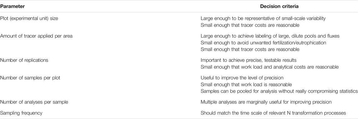
TABLE 1. Decision scheme for whole ecosystem¹⁵N tracer studies.

Tracer Application

Besides the amount of tracer to apply, addressed in the previous section, there are several other practical aspects connected to the application of the tracer. These are mainly: the method of application, the chemical form of the tracer and the timing. Their optimization always depends on the questions asked in these studies. In experiments with mineral fertilizers, tracers can be chosen in the same chemical form and applied mixed into the fertilizer. More questions arise in experiments with the aim of assessing the fate of atmospheric N deposition. In their meta-analysis, Templer et al. (2012) distinguish between three chemical forms (¹⁵NH₄¹⁵NO₃, ¹⁵NH₄⁺ or ¹⁵NO₃⁻) and between two application methods (to the canopy or to the soil). The choice of the chemical form depends on the local composition of the deposition that researchers want to trace. If it is possible to do so, applying ¹⁵NH₄⁺ and ¹⁵NO₃⁻ to separate plots leads to a better understanding of their respective short-term plant uptake and immobilization processes. Ammonium is retained much better in the soil than nitrate, by adsorption on clay and humus, and both ions also differ in their uptake by plants (Providoli et al., 2006; Feng et al., 2008; Liu et al., 2017). The preference of plants for these ions appears to be related to their mycorrhizal association (Goodale, 2017). Organic forms of N like glycine have mainly been tested in cold ecosystems where they may play a greater role in plant uptake (Sorensen et al., 2008; Dawes et al., 2017).

As long as the goal is to understand the fate of N from atmospheric deposition, applying the tracer over the canopy is the most representative method. In forests, this has been successfully done by helicopter (Dail et al., 2009). Due to the cost of this method (especially if the application has to be repeated over time), most studies are done by applying the tracer under the tree canopy, over the ground vegetation (Templer et al., 2012). This obviously does not allow for tracer uptake by tree foliage, a mechanism found for both broadleaves and needles, especially in young trees (Wilson and Tiley, 1998; Sparks, 2009; Nair et al., 2016). In contrast, application directly on or into the soil can be used to study plant uptake only via the roots.

The timing of tracer application is also a factor to be considered, as it is well known from agricultural crops that N availability should coincide with plant demand to maximize uptake. Atmospheric deposition, in contrast, has its own seasonality. In order to quantify the fate of N deposition over a year, it is thus advisable to follow a similar seasonality with the tracer, applying it in multiple small amounts. This was done, for example, in small headwater catchments by Providoli et al. (2005). They even noticed that applying the tracer at time of rain events led to more tracer appearing in leached nitrate than when the tracer was applied independent of the weather. This finding can be explained by preferential water flow through the soil during rain events, which hinders nitrate uptake. In experiments with roofs, deposition with a manipulated chemical composition was applied using automated sprinkler systems that simulated the actual rain events (Boxman et al., 1995; Lamersdorf and Borken, 2004; Feng et al., 2008). A single-dose tracer application, as sometimes performed, has the disadvantage that the obtained tracer partitioning is not representative of the actual seasonal dynamics.

A different approach is to follow the recycling of N within the ecosystem using labeled plant litter (Blumfield et al., 2004; Tonon et al., 2007; Hatton et al., 2012). For such experiments, labeled litter is first produced, typically by cultivating plants in pots with a ¹⁵N-enriched fertilizer. This prior step may be a reason why the application of ¹⁵N via plant litter is chosen relatively seldomly, despite its importance for understanding the release of N from decomposing plant litter and its incorporation into older soil organic matter.

Sampling and Calculations

Three Components to Determine Tracer Recovery

To calculate the tracer recovery in an ecosystem pool or flux, it is necessary to measure three variables: the tracer fraction, the element concentration and the total mass of the pool or flux.

The tracer fraction in a pool or flux, also called specific labeling, is calculated from an N mass balance. Without tracer, all N pools and fluxes already contain ¹⁵N at a natural abundance level. This means that measured ¹⁵N is partly native and partly stems from the tracer (see equations below). Three ¹⁵N fractional abundances thus enter the calculation: the abundance in the tracer itself, the natural (native) abundance in the pool or flux and the abundance coming from the tracer. These abundances can be measured by isotope-ratio mass spectrometry (IRMS). For a bulk analysis, the IRMS is usually coupled to an element analyzer in which the samples are completely oxidized. In this case, it can easily be combined with the analysis of ¹³C, but other configurations are possible according to the chemical compounds of interest (see some details in “Specific Ecosystem Pools and Fluxes” section).

Abundances can be quantified with a relative precision that deteriorates with increasing natural and experimental variability. Because the natural abundance is relatively constant through space and time, it requires few samples and analyses to achieve a sufficient precision. In the labeled pools and fluxes, in contrast, the ¹⁵N abundance varies because of inhomogeneity both in the tracer application (experimental imprecision) and in the N cycling processes (natural variability). To compensate for this variability, the labeled pools and fluxes should be sampled and analyzed with a higher intensity than the controls used for the determination of natural abundances. This is especially true in short-term studies, where N pools and fluxes are analyzed at a frequency of hours or days: at this time scale, the natural abundances usually do not show any measurable changes. If the ¹⁵N abundance in the pool remains much higher than its natural abundance, the latter may even be ignored in the calculation (see Eq. 4 below).

The N concentration in the pools or fluxes is usually measured in the same samples used to determine their ¹⁵N abundance, most of the time in the same mass spectrometry analysis. Because the mass spectrometer is optimized for measuring the ¹⁵N abundance and not necessarily the N concentration, a separate analysis may improve the precision and also make it possible to measure other chemical elements like carbon and sulfur.

The pool sizes or fluxes are often measured independently from the N and ¹⁵N analyses. The measurement techniques vary according to the nature of these pools or fluxes (e. g. soil, plants, water) and will, thus, be discussed in the following sections.

Calculation of Tracer Recovery

Methods for calculating tracer recovery have been described in many publications, but often with diverging or even mathematically improper notations. Equations (Providoli et al., 2005) are therefore recalled and completed here, using SI units and thus avoiding unnecessary conversion factors. Abundances of stable isotopes in samples are routinely expressed in the δ notation in relation to a standard (Eq. 1):

${\delta }^{15}\text{N}={\text{R}}_{\text{sample}}/{\text{R}}_{\text{standard}}-1(1)$

where R is defined as the molar fraction of the heavier to the lighter isotope, i.e. ¹⁵N/¹⁴N. δ values are essentially dimensionless and mostly expressed in ‰. For ¹⁵N, the standard is atmospheric N₂, with R_standard = 0.0036765. R_sample can be calculated by inverting Eq. 1 to Eq. 2:

${\text{R}}_{\text{sample}}=({\delta }^{15}{\text{N}}_{\text{sample}}+1)\cdot {\text{R}}_{\text{standard}}{=}^{15}{\text{N}}_{\text{sample}}{/}^{14}{\text{N}}_{\text{sample}}(2)$

For further calculations, we use the molar ratio to calculate the fractional abundance (Eq. 3):

$\text{F}=\text{R}/(\text{R}+1){=}^{15}\text{N}/{(}^{14}\text{N}{+}^{15}\text{N})(3)$

Equation 3 is given without subscripts because it applies to samples as well as to standard and reference material. Unfortunately, there are actually two definitions of δ coexisting in scientific publications. The second has the same form as Eq. 1 but with F instead of R, and thus uses F_standard = 0.003663. To avoid unnecessary confusion, we do not give this second equation explicitly. The F-based δ would actually be preferable because it makes calculations a bit easier, but IRMS laboratories typically use the R-based definition and report results in this form. Therefore, Eq. 2 and Eq. 3 should normally be used in calculations based on δ values from an IRMS laboratory. Double-checking this is still advisable.

In a next step (Eq. 4), fractional abundances are used to calculate the tracer fraction X_sample, defined as the molar ratio of tracer N to total N in a sample:

${\text{X}}_{\text{sample}}=({\text{F}}_{\text{sample}}-{\text{F}}_{\text{reference}})/({\text{F}}_{\text{tracer}}-{\text{F}}_{\text{reference}})(4)$

where F_reference is the fractional abundance in unlabeled samples and F_tracer is the abundance in the applied tracer (typically given as atom % by the producer). All equations so far are based on the number of atoms and not on their mass. For further calculations, we need amounts of N, which are typically obtained as masses (g) from IRMS laboratories. It is therefore necessary to convert these masses to moles (Eq. 5):

$\text{n}=\text{m}/\text{M}(5)$

where n is the molar quantity, m the mass and M the molar mass. Because of the different masses of the isotopes, the molar mass itself is not constant but needs to be calculated from the isotope fraction F (Eq. 6):

$\text{M}=14.003074\cdot (1-\text{F})+15.000109\cdot \text{F}=14.003074+0.997035\cdot \text{F}(6)$

Note that coefficients in Eq. 6 (in g mol⁻¹) are often rounded to the unit, i.e. to 14, 15 and 1, which affects the results only from the fifth significant digit onwards. Finally, the tracer recovery Z (tracer recovered in a pool or flux relative to the tracer applied) can be calculated (Eq. 7):

${\text{Z}}_{\text{pool}}={\text{X}}_{\text{sample}}·{\text{n}}_{\text{pool}}/{\text{n}}_{\text{tracer}}(7)$

where n_pool and n_tracer are the total amounts of N (in mol) in the pool and in the tracer, respectively. These amounts of N can be expressed per experimental unit (plot) or per area, but both should obviously be on the same basis. The tracer recovery Z_pool is usually expressed in %, but this is again only a transformation of units and thus not included in the SI-based equation.

In some studies, N masses were not transformed into molar quantities, i.e. N masses were used in Eq. 7 instead of N amounts in mol (Hauck and Bremner, 1976; Nadelhoffer and Fry, 1994). The resulting difference in terms of tracer recovery can be quantified. Substituting Eq. 5 and Eq. 6 into Eq. 7 gives:

${\mathrm{Z}}_{\text{pool}}={\mathrm{X}}_{\text{sample}}·{\mathrm{m}}_{\text{pool}}/{\mathrm{m}}_{\text{tracer}}·(14+{\mathrm{F}}_{\text{tracer}})/(14+{\mathrm{F}}_{\text{pool}})(8)$

So if tracer recovery is calculated using masses (m) instead of molar quantities (n), the resulting Z_pool differs from the true value by a factor (14 + F_tracer)/(14 + F_pool). In case of a highly enriched tracer (F_tracer ≈ 1) and small sample enrichments (F_pool << 1), this factor equals 15/14. This means that tracer recoveries are underestimated by about 7%.

Graphical Representation of ¹⁵N Recovery

In a tracer experiment, recovery in an N pool (Z in the above calculations) is proportional to the pool's size (n_pool) times its tracer fraction (X). This is illustrated graphically in Figure 1, which shows the results of two tracer experiments in a forest with experimental low and high N deposition (Wessel et al., 2021). The area of each rectangle represents the recovery in an N pool, with the vertical dimension indicating the size of the N pool and the horizontal dimension the tracer fraction. As the tracer application amounts differed between N deposition treatments, the x-axis scale differs among panels. In the figure it is apparent that some pools contributed considerably to the total tracer recovery because they were large, such as the mineral soil pools. Other pools, such as the aboveground vegetation and the LF1 layer, only made a small contribution to the total ¹⁵N recovery despite their relatively large tracer fraction because their N pool sizes were small.

FIGURE 1

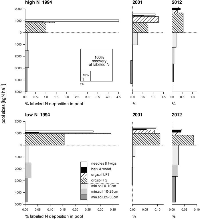
FIGURE 1. Size of each N pool against the presence of tracer in the pool in high and low N deposition plots in a Scots pine forest, one, eight and nineteen years after labeling. The area of each rectangle represents the recovery of ¹⁵N in that pool (expressed as the proportion of applied label, see legend in upper left panel). Please note that the x-axes for the high and the low N deposition treatments have different scales. Redrawn from Wessel et al. (2021).

Specific Ecosystem Pools and Fluxes

Soil

Much of the applied ¹⁵N tracer is typically recovered in the soil (Templer et al., 2012), and the accuracy of the total recovery thus largely depends on the accuracy of the soil analysis. Soil cores are typically taken according to sampling schemes similar to those used for other chemical analyses. These cores are then analyzed individually or combined to form composite samples. If present, undecomposed plant litter can be taken from the same cores and separated from the decomposing organic soil horizon. After this, the soil cores have to be cut according to their horizons. This step is crucial because it determines how well the obtained results will be comparable across plots, treatments, sampling times or even between different experiments and soil types. Cutting horizons by depth or along horizon borders is a matter of choice, as is the case of soil analyses in general. Working with horizons can facilitate interpretation of the results, but working with depths can be more reproducible across soil types. Apparent soil densities may show large spatial and temporal variations within a layer or horizon. For this reason, it is always advisable to measure the dry mass of each horizon in each sample. Relying on an average density can lead to gross errors, especially when this density is low and the soil tends to be compressed during coring.

If the mass, the N concentration and the tracer fraction are all measured from the same sample (corresponding to one or several cores), then the N recovery can also be calculated per sample before being averaged. This is better than calculating averages of the mass, N concentration and tracer fraction for two reasons. First, it allows a direct calculation of statistical parameters (standard deviation, standard error, confidence intervals) of the recovery. Second, it is not biased if the three variables are somehow correlated. For example, a sample having a higher N content (higher mass and/or higher N concentration) can be expected to have a lower tracer fraction due to dilution by the native N. In this case, averaging the tracer fractions would lead to an overestimation compared with averaging the tracer recoveries (Table 2). This leads to the following general advice: calculate averages of amounts, not of abundances or concentrations. If, for any reason, the mass, N concentration and tracer fraction are not measured in the same samples, then error propagation laws have to be used to estimate the standard error of the tracer recovery. In most such cases, correlations between the three components of the recovery are not known, and this prevents a proper calculation of error propagation. However, because pool mass, N concentration and tracer fraction are more likely to be negatively than positively correlated, a calculation without accounting for these correlations can be considered conservative.

TABLE 2

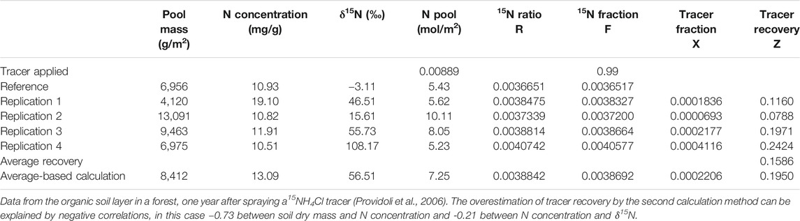
TABLE 2. Calculation of tracer recovery by averaging the recovery of single samples (replications) vs. the calculation based on average N concentrations and δ¹⁵N.

Soil Components

N is present in many different bio-physico-chemical forms in the soil. Besides calculating total tracer recovery in soil horizons, it is often interesting to determine in greater detail the forms in which the applied tracer is present. The most frequent goal of these analyses is to separate more or less stable fractions, which can store and release the tracer at different time scales. Typical methods are extraction (e.g. Providoli et al., 2006), hydrolysis (e.g. Morier et al., 2010) and density fractionation (e.g. Hatton et al., 2012; Kramer et al., 2017, on natural ¹⁵N abundance). The fumigation-extraction method (Brookes et al., 1985) plays a specific role as it allows the estimation of tracer recovery in soil microorganisms. It is not our goal here to examine the advantages and limitations of these methods, which are not directly related to isotopes. The analysis of aqueous solutions obtained from extractions will be treated in “Water” section, along with the analysis of natural water samples.

In the context of ¹⁵N tracer experiments, the recovery rate of extraction or separation methods always plays a central role, as it also affects the recovery rate of the tracer. Correction factors are often applied, for example to estimate microbial N from the fumigation-extraction method. Applying the same factor to the tracer is always questionable and should in any case be interpreted with caution. Further, one of the greatest challenges is certainly to relate fractions empirically obtained by analyses to pools defined conceptually or implemented practically in ecosystem models.

Roots

Fine roots (<2 mm as the standard definition) are usually taken from the same soil cores as used for soil analysis. Depending on the morphology of the roots and on the soil structure, this task can be very time consuming. This is especially the case for dense root systems of Gramineae. In some cases, it is easier to work with separate cores and to wash the roots free of soil with water, subsequently calculating tracer recovery in the root-free soil as a difference.

Coarse roots, especially coarse tree-roots, can rarely be sampled quantitatively by soil coring. A separate estimation of their dry mass can improve the results, but the accuracy is essentially limited by the difficulty in accessing root systems. Systematic sampling often requires a considerable amount of digging, i.e. more destructive sampling. If available, allometric estimations based on aboveground parameters may be sufficient to estimate the dry mass of coarse roots. As the tracer fraction and pool size are not estimated from the same samples, the accuracy of the tracer recovery has to be estimated by error propagation laws, and, as a consequence, possible correlations between the two remain unnoticed. Another consequence of using allometric relationships is that the spatial variation in the dry mass is practically impossible to determine, and is generally ignored in calculations and statistical tests.

Ground Vegetation

The ground vegetation comprises mosses and aboveground parts of herbaceous vegetation and of shrubs. Except for taller shrubs, ground vegetation is best analyzed by quantitatively harvesting patches. The number and size of the patches must be chosen according to the homogeneity of the vegetation cover. In ecosystems with only a few plant species, the individual species can be weighed and analyzed separately. In species-rich systems, functional groups may be considered, for example separating mosses, monocotyledons and dicotyledons. If a species or a functional group is absent from a sample, then its tracer fraction and N concentration are missing data. Its tracer recovery, however, is not missing data but rather zero. Treating it as missing data would mean overestimating the average recovery by systematically removing all zero values. Again, to avoid bias in the recovery calculation, the same rule as for the soil (see above) should be applied: amounts can be averaged, whereas abundances and concentrations should not.

Trees

The aboveground parts of large shrubs and trees can rarely be harvested quantitatively to analyze their tracer recovery. Just as in the case of coarse roots, the biomass of their different parts has to be estimated by allometric relationships: foliage, branches and trunks (bark, wood). The corresponding pools are sampled and analyzed separately. Wood is often difficult to analyze because of its high C/N ratio (Savard et al., 2020), meaning that its combustion for mass spectrometry produces much CO₂ but little N. Wood must be finely ground before analysis because the combustion of even tiny wood chips is not fast enough. In some species, it has been observed that tracer N also enters older wood (Tomlinson et al., 2014). It is thus important to take wood cores that go deep enough into the trunks. In spruce trees, for example, tree rings from at least the last 30 years should be analyzed, but rings can be grouped (Schleppi et al., 1999). Analyzing wood from different heights above the ground has also been tested but does not appear to be necessary (Nadelhoffer et al., 2004). The wood mass of each ring or ring group is then calculated from the ring widths and wood densities, and from the size of the trees. A model for the shape of the tree species is therefore necessary (for example a simple conical shape). For the diagnostic of nutrient status, tree foliage is typically taken from the top, sunlight-exposed part of the crowns, which enables comparisons between trees and between stands. For a mass balance, however, it is essential to remember that shade foliage can be very different from sunlit foliage. This is true for its chemical composition but also especially for its morphological parameters, with shade foliage having a lower specific mass (less dry matter per area). The specific leaf mass is required in the calculation of the total mass of foliage based on indirect measurements of the leaf area index (leaf area per ground area). It is thus advisable to sample foliage from different heights within a forest canopy.

Water

For the analysis of soluble N compounds in water samples or soil extracts, it is necessary to separate them from the water, which is often time consuming. For the combined analysis of ¹⁵N and ¹⁸O in nitrate, we refer to the extensive publication by Kendall et al. (2007). As long as no other isotope has to be measured (e.g. ¹⁸O in nitrate), the method of ammonia diffusion is well established, giving good recovery rates and sufficient precision (Schleppi et al., 2006a). With this method, it is possible to determine the isotope fraction in inorganic N. This is achieved directly for ammonium and for nitrate after its reduction to ammonium. Total dissolved ¹⁵N can be measured by first lyophilizing the water samples, then analyzing the residue by IRMS. The ¹⁵N fraction in dissolved organic N (DON) can be calculated as the difference between total N and inorganic N (e.g. Providoli et al., 2006). If there is much more tracer in inorganic N than in DON, however, this calculation becomes too inaccurate.

In contrast to soil or plant pools, water can be highly mobile in an ecosystem, in which case its fluxes must be considered. This requires more frequent sampling and appropriate methods to integrate element fluxes based on discrete analyses (Schleppi et al., 2006b). In hydrologically defined catchments, dissolved N compounds leaving the ecosystem can be determined by quantifying and sampling the runoff. For vertical movements of water-dissolved N in the soil, water fluxes need to be modeled (Koopmans et al., 1996; Gundersen, 1998; Feng et al., 2008). The application and constraints of such an approach are not different than for dissolved compounds in general and thus will not be detailed here (Tiktak and Van Grinsven, 1995).

Longitudinal Studies and Modeling

Longitudinal studies involve the repeated sampling and analysis of pools and fluxes over several years or even decades. Compared with short-term studies with a time scale of days, long-term studies pose some specific challenges and opportunities. The long-term fate of ¹⁵N tracers is especially useful to assess the effect of slow changes, as brought about by atmospheric deposition (Veerman et al., 2020; Wessel et al., 2021) or climate change (Cheng et al., 2019). Interpretation of long-term tracer experiments can be a challenge, but can be improved by the use of models (Currie, 2007). These vary from simple mixing models to derive the N dynamics of one tracer experiment (Gerzabek et al., 2004) to complete ecosystem models (Van Dam and Van Breemen, 1995; Currie et al., 2004). The latter are complex models, including many ecosystem processes such as photosynthesis, substrate allocation, litter production, soil organic carbon transformations, and water and solute flow. Such models, however, have only been applied to field experiments in a few cases (Koopmans and Van Dam, 1998; Currie et al., 2004; Krause et al., 2012), as all the different processes in the model have to be parameterized and calibrated before the model can be put to use. An alternative to these models is the approach used by Rastetter et al. (2005), in which an already existing model is used for the simulation of the N dynamics, after which a second model just adds the ¹⁵N dynamics to the total N simulation results from the first model. As the ¹⁵N does not affect the N transformations or any other process in the ecosystem, its dynamics can be calculated afterward. Another approach is to mimic ¹⁵N dynamics in models by running such a model twice, adding a small amount of additional N into the N deposition input stream representing the tracer during the second model run (Thomas et al., 2013; Cheng et al., 2019). As these models have a broader application than just for the modeling of ¹⁵N tracer, the effort needed to get them to produce meaningful output may be less.

As an example of a simple model application, we show here how the analysis of ¹⁵N in tree needles and litter can help to understand the plant uptake of N brought about by atmospheric deposition. The data (Figure 2) are from a long-term NH₄NO₃ addition to a subalpine coniferous forest where the treatment was labeled on both ions (¹⁵NH₄¹⁵NO₃) during the first year (Schleppi et al., 1999). Needles of conifers can be separated according to their age. Here, we sampled five cohorts and repeated the measurements for nine years. Litter was also collected, with about two thirds of this material being old needles. The N translocation model used with these data is based on three plant pools (Figure 2): the needles (divided into seven age classes), a mobile N pool in woody tissues and bark, and the N immobilized in such tissues. The uptake from the soil, translocation within the plant and N loss by litterfall were the considered fluxes, with rates calibrated by fitting the model to the available data. These rates are all depicted in Figure 3. The best fit explained R² = 91% of the variance in the δ¹⁵N measurements. Besides the incorporation of new N into growing needles (cohort 1, marginally also cohort 2) and retranslocation out of senescing needles (cohorts 4–7), relatively large exchanges between the different cohorts via the mobile N pool had to be taken into account in order to achieve the observed partitioning of tracer across the different needle age classes. The modeled tracer N uptake by the trees is shown as bars in Figure 3. This time-course contrasts very much with the rapid disappearance of ¹⁵N in nitrate leached from this forest (Providoli et al., 2005; Schleppi et al., 2017). On the other hand, ¹⁵N available to trees decreases markedly from year to year while tracer in the bulk soil remains quite stable for decades, as observed in this experiment as well as in three other experimental forests across Europe (Veerman et al., 2020). This clearly shows that different N pools with different turnover times are involved. A simple model like the one considered here obviously cannot unravel the different processes taking place in the soil itself, but it shows the potential value of combining longitudinal tracer studies with ecosystem models.

FIGURE 2

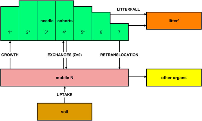
FIGURE 2. Simple model used to describe the translocation of ¹⁵N tracer in coniferous trees with several needle age classes (cohorts). Measured N pool and ¹⁵N abundances are indicated by stars.

FIGURE 3

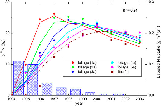
FIGURE 3. ¹⁵N abundances in Norway spruce needle cohorts and in litterfall in an N addition experiment in which a¹⁵NH₄¹⁵NO₃ tracer was applied during the initial year (Schleppi et al., 1999). Dots represent measurements and lines are modeled δ¹⁵N values. The modeled tracer uptake by the trees is shown as bars.

Challenges and Opportunities

According to Templer et al. (2012), most ¹⁵N studies in terrestrial ecosystems show a total tracer recovery well below 100%. Grasslands show even less recovery than forests in spite of the fact that an herbaceous vegetation is much easier to sample quantitatively. Some fluxes often remain unaccounted for in such studies, especially volatilization immediately after application, denitrification, grazing and lateral fluxes out of the plots. N leaching (mainly as nitrate but also as DON) is usually not directly measured but calculated by multiplying concentrations in soil water under the rooting zone by water infiltration at this level. This approach neglects preferential flow and may thus lead to an underestimation of the leaching flux. While lateral fluxes can be minimized by labeling also borders around the sampled plots (mainly above the plot if it is on a slope), all other processes are relatively difficult to capture and thus remain a challenge for future studies.

¹⁵N tracer studies in terrestrial ecosystems, especially in forests, have been used to constrain global climate models (Nadelhoffer et al., 1999; Cheng et al., 2019). This kind of application has been criticized because N uptake by tree canopies is not taken into account when ¹⁵N tracer is applied under tree crowns (Sievering, 1999; Nair et al., 2016). While the uptake of sprayed tracer by foliage of small trees has been well documented (Sparks, 2009), the magnitude of this process is still not really quantified for trees in their forest environment, especially considering the difficulty of reproducing experimentally the N deposition brought by natural rain events. Towers built in forests for research purposes may give opportunities to conduct realistic tracer experiments where ¹⁵N could be sprayed over trees specifically during rain events.

Data Availability Statement

The model and dataset presented in this study are available upon request from the corresponding author.

Author Contributions

PS planned and wrote large parts of the manuscript. WWW wrote other parts. Both authors edited the manuscript.

Conflict of Interest

The authors declare that the research was conducted in the absence of any commercial or financial relationships that could be construed as a potential conflict of interest.

Acknowledgments

The European Science Foundation funded a visit by W. W. Wessel to the Swiss Federal Institute for Forest, Snow and Landscape Research (ClimMani Exchange Grant 2012). We thank Dr M. Dawes for language editing of the manuscript.

References

Björkman, E., Lundeberg, G., and Nömmik, H. (1967). Distribution and Balance of N¹⁵ Labeled Fertilizer Nitrogen Applied to Young Pine Trees (Pinus silvestris L.). Stud. For. Suec. 48, 5–23.

Google Scholar

Blumfield, T. J., Xu, Z., Mathers, N. J., and Saffigna, P. G. (2004). Decomposition of Nitrogen-15 Labeled Hoop Pine Harvest Residues in Subtropical Australia. Soil Sci. Soc. Am. J. 68, 1751–1761. doi:10.2136/sssaj2004.1751

CrossRef Full Text | Google Scholar

Boxman, A. W., Van Dam, D., Van Dijk, H. F. G., Hogervorst, R., and Koopmans, C. J. (1995). Ecosystem Responses to Reduced Nitrogen and Sulphur Inputs into Two Coniferous Forest Stands in the Netherlands. For. Ecol. Manage. 71, 7–29. doi:10.1016/0378-1127(94)06081-S

CrossRef Full Text | Google Scholar

Brookes, P. C., Kragt, J. F., Powlson, D. S., and Jenkinson, D. S. (1985). Chloroform Fumigation and the Release of Soil Nitrogen: The Effects of Fumigation Time and Temperature. Soil Biol. Biochem. 17, 831–835. doi:10.1016/0038-0717(85)90143-9

CrossRef Full Text | Google Scholar

Cheng, S. J., Hess, P. G., Wieder, W. R., Thomas, R. Q., Nadelhoffer, K. J., Vira, J., et al. (2019). Decadal Fates and Impacts of Nitrogen Additions on Temperate Forest Carbon Storage: a Data-Model Comparison. Biogeosciences 16, 2771–2793. doi:10.5194/bg-16-2771-2019

CrossRef Full Text | Google Scholar

Currie, W. S., Nadelhoffer, K. J., and Aber, J. D. (2004). Redistributions of ¹⁵N Highlight Turnover and Replenishment of Mineral Soil Organic N as a Long-Term Control on Forest C Balance. For. Ecol. Manage. 196, 109–127. doi:10.1016/j.foreco.2004.03.015

CrossRef Full Text | Google Scholar

Currie, W. S. (2007). “Modeling the Dynamics of Stable-Isotope Ratios for Ecosystem Biogeochemistry,” in Stable Isotopes in Ecology and Environmental Science. Editors R. Michener, and K. Lajtha 2nd ed. (Malden, MA, USA: Blackwell), 450–479. doi:10.1002/9780470691854.ch13

CrossRef Full Text | Google Scholar

Dail, D. B., Hollinger, D. Y., Davidson, E. A., Fernandez, I., Sievering, H. C., Scott, N. A., et al. (2009). Distribution of Nitrogen-15 Tracers Applied to the Canopy of a Mature Spruce-Hemlock Stand, Howland, Maine, USA. Oecologia 160, 589–599. doi:10.1007/s00442-009-1325-x

PubMed Abstract | CrossRef Full Text | Google Scholar

Dawes, M. A., Schleppi, P., and Hagedorn, F. (2017). The Fate of Nitrogen Inputs in a Warmer Alpine Treeline Ecosystem: a ¹⁵N Labelling Study. J. Ecol. 105, 1723–1737. doi:10.1111/1365-2745.12780

CrossRef Full Text | Google Scholar

Erisman, J. W., van Grinsven, H., Grizzetti, B., Bouraoui, F., Powlson, D., Sutton, M. A., et al. (2011). “The European Nitrogen Problem in a Global Perspective,” in The European Nitrogen Assessment: Sources, Effects and Policy Perspectives. Editors M. A. Sutton, C. M. Howard, J. W. Erisman, G. Billen, A. Bleekeret al. (Cambridge: Cambridge University Press), 9–31. url: http://www.nine-esf.org/files/ena_doc/ENA_pdfs/ENA_c2.pdf

Google Scholar

Feng, Z., Brumme, R., Xu, Y.-J., and Lamersdorf, N. (2008). Tracing the Fate of Mineral N Compounds Under High Ambient N Deposition in a Norway Spruce Forest at Solling/Germany. For. Ecol. Manage. 255, 2061–2073. doi:10.1016/j.foreco.2007.12.049

CrossRef Full Text | Google Scholar

Fry, B. (2006). Stable Isotope Ecology. New York: Springer. doi:10.1007/0-387-33745-8

CrossRef Full Text

Gardner, J. B., and Drinkwater, L. E. (2009). The Fate of Nitrogen in Grain Cropping Systems: a Meta-Analysis of ¹⁵N Field Experiments. Ecol. Appl. 19, 2167–2184. doi:10.1890/08-1122.1

PubMed Abstract | CrossRef Full Text | Google Scholar

Gerzabek, M. H., Haberhauer, G., Stemmer, M., Klepsch, S., and Haunold, E. (2004). Long-Term Behaviour of ¹⁵N in an Alpine Grassland Ecosystem. Biogeochem. 70, 59–69. doi:10.1023/B:BIOG.0000049336.84556.62

CrossRef Full Text | Google Scholar

Goodale, C. L. (2017). Multiyear Fate of a ¹⁵N Tracer in a Mixed Deciduous Forest: Retention, Redistribution, and Differences by Mycorrhizal Association. Glob. Change Biol. 23, 867–880. doi:10.1111/gcb.13483

PubMed Abstract | CrossRef Full Text | Google Scholar

Gundersen, P. (1998). Effects of Enhanced Nitrogen Deposition in a Spruce Forest at Klosterhede, Denmark, Examined by Moderate NH₄NO₃ Addition. For. Ecol. Manage. 101, 251–268. doi:10.1016/S0378-1127(97)00141-2

CrossRef Full Text | Google Scholar

Hatton, P.-J., Kleber, M., Zeller, B., Moni, C., Plante, A. F., Townsend, K., et al. (2012). Transfer of Litter-Derived N to Soil Mineral-Organic Associations: Evidence from Decadal ¹⁵N Tracer Experiments. Org. Geochem. 42, 1489–1501. doi:10.1016/j.orggeochem.2011.05.002

CrossRef Full Text | Google Scholar

Hauck, R. D., and Bremner, J. M. (1976). Use of Tracers for Soil and Fertilizer Nitrogen Research. Adv. Agron. 28, 219–266. doi:10.1016/S0065-2113(08)60556-8

CrossRef Full Text | Google Scholar

Hauck, R. D., Bartholomew, W. V., Bremner, J. M., Broadbent, F. E., Cheng, H. H., Edwards, A. P., et al. (1972). Use of Variations in Natural Nitrogen Isotope Abundance for Environmental Studies: a Questionable Approach. Science 177, 453–456. doi:10.1126/science.177.4047.453

PubMed Abstract | CrossRef Full Text | Google Scholar

Kendall, C., Elliott, E. M., and Wankel, S. D. (2007). “Tracing Anthropogenic Inputs of Nitrogen to Ecosystems,” in Stable Isotopes in Ecology and Environmental Science. Editors R. Michener and K. Lajtha. 2nd Edn. (Malden, MA:Blackwell), 375–449. doi:10.1002/9780470691854.ch12

PubMed Abstract | CrossRef Full Text | Google Scholar

Koopmans, C. J., and Van Dam, D. (1998). Modelling the Impact of Lowered Atmospheric Nitrogen Deposition on a Nitrogen Saturated Forest Ecosystem. Water Air Soil Pollut. 104, 181–203. doi:10.1023/A:1004992614988

CrossRef Full Text | Google Scholar

Koopmans, C. J., Tietema, A., and Boxman, A. W. (1996). The Fate of ¹⁵N Enriched Throughfall in Two Coniferous Forest Stands at Different Nitrogen Deposition Levels. Biogeochem. 34, 19–44. doi:10.1007/BF02182953

CrossRef Full Text | Google Scholar

Kramer, M. G., Lajtha, K., and Aufdenkampe, A. K. (2017). Depth Trends of Soil Organic Matter C:N and ¹⁵N Natural Abundance Controlled by Association with Minerals. Biogeochem. 136, 237–248. doi:10.1007/s10533-017-0378-x

CrossRef Full Text | Google Scholar

Krause, K., Providoli, I., Currie, W. S., Bugmann, H., and Schleppi, P. (2012). Long-Term Tracing of Whole Catchment ¹⁵N Additions in a Mountain Spruce Forest: Measurements and Simulations with the TRACE Model. Trees 26, 1683–1702. doi:10.1007/s00468-012-0737-0

CrossRef Full Text | Google Scholar

Lamersdorf, N. P., and Borken, W. (2004). Clean Rain Promotes Fine Root Growth and Soil Respiration in a Norway Spruce Forest. Glob. Change Biol. 10, 1351–1362. doi:10.1111/j.1365-2486.2004.00811.x

CrossRef Full Text | Google Scholar

Liu, J., Peng, B., Xia, Z., Sun, J., Gao, D., Dai, W., et al. (2017). Different Fates of Deposited NH₄⁺ and NO₃⁻ in a Temperate Forest in Northeast China: a ¹⁵N Tracer Study. Glob. Change Biol. 23, 2441–2449. doi:10.1111/gcb.13533

PubMed Abstract | CrossRef Full Text | Google Scholar

Morier, I., Schleppi, P., Saurer, M., Providoli, I., and Guenat, C. (2010). Retention and Hydrolysable Fraction of Atmospherically Deposited Nitrogen in Two Contrasting Forest Soils in Switzerland. Eur. J. Soil Sci. 61, 197–206. doi:10.1111/j.1365-2389.2010.01226.x

Google Scholar

Nadelhoffer, K. J., and Fry, B. (1994). “Nitrogen Isotope Studies in Forest Ecosystems,” in Stable Isotopes in Ecology and Environmental Science. Editors K. Lajtha, and R. H. Michener (Oxford: Blackwell), 22–44.

Google Scholar

Nadelhoffer, K. J., Emmett, B. A., Gundersen, P., Kjønaas, O. J., Koopmans, C. J., Schleppi, P., et al. (1999). Nitrogen Deposition Makes a Minor Contribution to Carbon Sequestration in Temperate Forests. Nature 398, 145–148. doi:10.1038/18205

CrossRef Full Text | Google Scholar

Nadelhoffer, K. J., Colman, B. P., Currie, W. S., Magill, A., and Aber, J. D. (2004). Decadal-Scale Fates of Tracers Added to Oak and Pine Stands Under Ambient and Elevated N Inputs at the Harvard Forest (USA). For. Ecol. Manage. 196, 89–107. doi:10.1016/j.foreco.2004.03.014

CrossRef Full Text | Google Scholar

Nair, R. K. F., Perks, M. P., Weatherall, A., Baggs, E. M., and Mencuccini, M. (2016). Does Canopy Nitrogen Uptake Enhance Carbon Sequestration by Trees? Glob. Change Biol. 22, 875–888. doi:10.1111/gcb.13096

CrossRef Full Text | Google Scholar

Nömmik, H. (1966). The Uptake and Translocation of Fertilizer N¹⁵ in Young Trees of Scots Pine and Norway Spruce. Stud. For. Suec. 35, 1–18.

Google Scholar

Providoli, I., Bugmann, H., Siegwolf, R., Buchmann, N., and Schleppi, P. (2005). Flow of Deposited Inorganic N in Two Gleysol-Dominated Mountain Catchments Traced with ¹⁵NO₃⁻ and ¹⁵NH₄⁺. Biogeochem. 76, 453–475. doi:10.1007/s10533-005-8124-1

CrossRef Full Text | Google Scholar

Providoli, I., Bugmann, H., Siegwolf, R., Buchmann, N., and Schleppi, P. (2006). Pathways and Dynamics of ¹⁵NO₃⁻ and ¹⁵NH₄⁺ Applied in a Mountain Picea abies forest and in a Nearby Meadow in Central Switzerland. Soil Biol. Biochem. 38, 1645–1657. doi:10.1016/j.soilbio.2005.11.019

CrossRef Full Text | Google Scholar

Rastetter, E. B., Kwiatkowski, B. L., and McKane, R. B. (2005). A Stable Isotope Simulator that Can Be Coupled to Existing Mass Balance Models. Ecol. Appl. 15, 1772–1782. doi:10.1890/04-0643

CrossRef Full Text | Google Scholar

Savard, M. M., Marion, J., and Bégin, C. (2020). Nitrogen Isotopes of Individual Tree-Ring Series - The Validity of Middle- to Long-Term Trends. Dendrochronologia 62, 125726. doi:10.1016/j.dendro.2020.125726

CrossRef Full Text | Google Scholar

Schleppi, P., Bucher-Wallin, L., Siegwolf, R., Saurer, M., Muller, N., and Bucher, J. B. (1999). Simulation of Increased Nitrogen Deposition to a Montane Forest Ecosystem: Partitioning of the Added ¹⁵N. Water Air Soil Pollut. 116, 129–134. doi:10.1023/A:1005206927764

CrossRef Full Text | Google Scholar

Schleppi, P., Bucher-Wallin, I., Saurer, M., Jäggi, M., and Landolt, W. (2006a). Citric Acid Traps to Replace Sulphuric Acid in the Ammonia Diffusion of Dilute Water Samples for ¹⁵N Analysis. Rapid Commun. Mass. Spectrom. 20, 629–634. doi:10.1002/rcm.2351

PubMed Abstract | CrossRef Full Text | Google Scholar

Schleppi, P., Curtaz, F., and Krause, K. (2017). Nitrate Leaching From a Sub-Alpine Coniferous Forest Subjected to Experimentally Increased N Deposition for 20 Years, and Effects of Tree Girdling and Felling. Biogeochem. 134, 319–335. doi:10.1007/s10533-017-0364-3

PubMed Abstract | CrossRef Full Text | Google Scholar

Schleppi, P., Waldner, P. A., and Fritschi, B. (2006b). Accuracy and Precision of Different Sampling Strategies and Flux Integration Methods for Runoff Water: Comparisons Based on Measurements of the Electrical Conductivity. Hydrol. Process. 20, 395–410. doi:10.1002/hyp.6057

CrossRef Full Text | Google Scholar

Schleppi, P., Körner, C., and Klein, T. (2019). Increased Nitrogen Availability in the Soil Under Mature Picea abies Trees Exposed to Elevated CO₂ Concentrations. Front. For. Glob. Change 2, 59. doi:10.3389/ffgc.2019.00059

CrossRef Full Text | Google Scholar

Schlesinger, W. H. (2009). On the Fate of Anthropogenic Nitrogen. Proc. Natl. Acad. Sci. USA 106, 203–208. doi:10.1073/pnas.0810193105

CrossRef Full Text | Google Scholar

Sievering, H. (1999). Nitrogen Deposition and Carbon Sequestration. Nature 400, 629–630. doi:10.1038/23176

CrossRef Full Text | Google Scholar

Sorensen, P. L., Michelsen, A., and Jonasson, S. (2008). Ecosystem Partitioning of ¹⁵N-Glycine After Long-Term Climate and Nutrient Manipulations, Plant Clipping and Addition of Labile Carbon in a Subarctic Heath Tundra. Soil Biol. Biochem. 40, 2344–2350. doi:10.1016/j.soilbio.2008.05.013

CrossRef Full Text | Google Scholar

Sparks, J. P. (2009). Ecological Ramifications of the Direct Foliar Uptake of Nitrogen. Oecologia 159, 1–13. doi:10.1007/s00442-008-1188-6

PubMed Abstract | CrossRef Full Text | Google Scholar

Templer, P. H., Mack, M. C., Iii, F. S. C., Christenson, L. M., Compton, J. E., Crook, H. D., et al. (2012). Sinks for Nitrogen Inputs in Terrestrial Ecosystems: a Meta-Analysis of ¹⁵N Tracer Field Studies. Ecology 93, 1816–1829. doi:10.1890/11-1146.1

PubMed Abstract | CrossRef Full Text | Google Scholar

Thomas, R. Q., Zaehle, S., Templer, P. H., and Goodale, C. L. (2013). Global Patterns of Nitrogen Limitation: Confronting Two Global Biogeochemical Models with Observations. Glob. Change Biol. 19, 2986–2998. doi:10.1111/gcb.12281

PubMed Abstract | CrossRef Full Text | Google Scholar

Tiktak, A., and Van Grinsven, H. J. M. (1995). Review of Sixteen Forest-Soil-Atmosphere Models. Ecol. Model. 83, 35–53. doi:10.1016/0304-3800(95)00081-6

CrossRef Full Text | Google Scholar

Tomlinson, G., Siegwolf, R. T. W., Buchmann, N., Schleppi, P., Waldner, P., and Weber, P. (2014). The Mobility of Nitrogen Across Tree-Rings of Norway Spruce (Picea abies L.) and the Effect of Extraction Method on Tree-Ring δ¹⁵N and δ¹³C Values. Rapid Commun. Mass. Spectrom. 28, 1258–1264. doi:10.1002/rcm.6897

PubMed Abstract | CrossRef Full Text | Google Scholar

Tonon, G., Ciavatta, C., Solimando, D., Gioacchini, P., and Tagliavini, M. (2007). Fate of ¹⁵N Derived from Soil Decomposition of Abscised Leaves and Pruning Wood From Apple (Malus domestica) Trees. Soil Sci. Plant Nutr. 53, 78–85. doi:10.1111/j.1747-0765.2007.00112.x

CrossRef Full Text | Google Scholar

Van Dam, D., and Van Breemen, N. (1995). NICCCE: a Model for Cycling of Nitrogen and Carbon Isotopes in Coniferous Forest Ecosystems. Ecol. Model. 79, 255–275. doi:10.1016/0304-3800(94)00184-J

CrossRef Full Text | Google Scholar

Veerman, L., Kalbitz, K., Gundersen, P., Kjønaas, J., Moldan, F., Schleppi, P., et al. (2020). The Long-Term Fate of Deposited Nitrogen in Temperate Forest Soils. Biogeochem. 150, 1–15. doi:10.1007/s10533-020-00683-6

CrossRef Full Text | Google Scholar

Wessel, W. W., and Tietema, A. (1992). Calculating Gross N Transformation Rates of ¹⁵N Pool Dilution Experiments With Acid Forest Litter: Analytical and Numerical Approaches. Soil Biol. Biochem. 24, 931–942. doi:10.1016/0038-0717(92)90020-X

CrossRef Full Text | Google Scholar

Wessel, W. W., Boxman, A. W., Cerli, C., van Loon, E. E., and Tietema, A. (2021). Long-Term Stabilization of ¹⁵N-Labeled Experimental NH₄⁺ Deposition in a Temperate Forest Under High N Deposition. Sci. Total Environ. 768, 144356. doi:10.1016/j.scitotenv.2020.144356

PubMed Abstract | CrossRef Full Text | Google Scholar

Wilson, E. J., and Tiley, C. (1998). Foliar Uptake of Wet-Deposited Nitrogen by Norway Spruce. Atmos. Environ. 32, 513–518. doi:10.1016/S1352-2310(97)00042-3

CrossRef Full Text | Google Scholar

Wright, R. F., and Dise, N. B. (1992). The NITREX Project (Nitrogen Saturation Experiments). Ecosyst. Res. Rep. 2. Brussels: Commission of the European Communitiesurl: https://op.europa.eu/en/publication-detail/-/publication/53885773-40dc-47d8-87d7-a28dc793153a/language-en

Google Scholar

Zhang, Z., Yuan, Y., Liu, Q., and Yin, H. (2019). Plant Nitrogen Acquisition From Inorganic and Organic Sources Via Root and Mycelia Pathways in Ectomycorrhizal Alpine Forests. Soil Biol. Biochem. 136, 107517. doi:10.1016/j.soilbio.2019.06.013

CrossRef Full Text | Google Scholar