Evaluating Asymmetric Approaches to the Estimation of Standard Uncertainties for Emission Factors in the Fuel Sector of Costa Rica

Introduction

Costa Rica is recognized worldwide as a pioneer in environmental protection and the fight against climate change (UN Environment Programme, 2019). Its efforts to achieve high recovery of its forest cover (Allen and Padgett-Vásquez, 2017), ecotourism as a key component of its economy (Courvisanos and Ameeta, 2006) and an electricity grid that is almost 100 % renewable (ICE Group, 2020) stand out. The new environmental challenge for Costa Rica involves its fossil-fueled transportation sector that generates large amounts of emissions and a variety of other problems (Fendt, 2017). In recent years the government of Costa Rica has launched national policies and plans that seek to decarbonize its economy (Government of Costa Rica, 2019), including its current transportation system and the environmental impact it generates. To achieve the success of these policies, it is essential to have precise and reliable data that allow the correct quantification of measures taken and guarantee the success of environmental efforts in favor of its conservation.

Measurement uncertainty, referred in this study simply as “uncertainty” and defined as the doubt about the true value of a quantity that remains after making that measurement or estimation, is the best quality parameter of any measurement or estimation and reflects the impossibility of knowing exactly its value (Joint Committee for Guides in Metrology [JCGM], 2008). Among the accepted methodologies for estimating uncertainty, the application of the law of propagation of uncertainty or Gauss’s formula included in the Guide to the Expression of Uncertainty in Measurement (GUM) stands out. This methodology is based on modeling an output quantity y as a known function of several input quantities and handles the uncertainties associated with the input quantities by modeling them as random variables. This approach uses the standard deviations of these random variables and their correlations to produce an approximate evaluation of the standard (measurement) uncertainty u_y, a measurement uncertainty expressed as a standard deviation associated to the output quantity y (Joint Committee for Guides in Metrology [JCGM], 2012). It should be highlighted that the conventional technique described in the GUM does not require necessarily that probability distributions of the input quantities to be symmetrical (Possolo et al., 2019).

In the context of greenhouse gas (GHG) inventories, uncertainty evaluation was initially considered as a non-mandatory requirement by ISO 14064-1 (2006), the main international standard for GHG quantification and reporting by organizations. Thus, the implementation of uncertainty estimates in GHG inventories has not yet been covered by many organizations that have already quantified emissions and mitigated their impact on the environment, depriving them of this measure of quality that strengthens the confidence of their results. Nevertheless, uncertainty in GHG inventories has been pointed as a key component to consider (Rypdal and Winiwater, 2001; EPA, 2002; Jonas et al., 2010) and several studies have been developed regarding this topic, including EPA (1996), Ritter et al. (2010); Milne et al. (2015), and Solazzo et al. (2020). With the publication of the new version of ISO 14064-1 (2018), uncertainty assessment takes on a new dimension by becoming a mandatory requirement. This conjuncture added to Costa Rican national scaled efforts to include uncertainty assessment through the National Carbon Neutrality Program (PPCN, by its Spanish acronym), has aroused national interest in the application of uncertainty estimation methodologies in GHG quantification (DCC and PMR, 2020; DCC and LCM, 2020).

A common scenario found in GHG inventories is the indirect quantification of emissions, where emissions are not measured directly as an amount of gas released into the atmosphere. Instead, emissions (E) are estimated from other data values associated with the activity that cause the emission (d) and emission factors (f) that relate these data to the amount of gas emitted, as shown in Equation (1). Emissions from energy consumption are a typical example of indirect quantification, where the emissions from e.g., a furnace can be estimated from the amount of fuel consumed and an emission factor that relates the liters of fuel with the amount of GHG released by the combustion process.

$E=d\cdot f(1)$

Following the application of Gauss’s formula (Joint Committee for Guides in Metrology [JCGM], 2008; Possolo and Iyer, 2017) to Equation (1), the approximate standard uncertainty of E (u_E) can be easily estimated from the values and standard uncertainties of d (u_d) and f (u_f), according to Equation (2).

$u_E=E\sqrt{{\left(\frac{u_d}{d}\right)}^2+{\left(\frac{u_f}{f}\right)}^2}(2)$

However, a significant limitation has been found by users when quantifying u_f since the literature usually includes references to asymmetric ranges of variation when describing the behavior of emission factors (Intergovernmental Panel on Climate Change [IPCC], 2000, 2006), including the official database of Costa Rican emission factors (IMN, 2020). This is attributable to the observed behavior when studying these factors, which usually present important dispersions depending on the study conditions. Small values are frequently found but relatively high values are plausible too, making asymmetry the commonly encountered behavior (Bharvirkar, 1999; Frey, 2007). Furthermore, the problem of propagating uncertainties expressed asymmetrically is not addressed in the GUM and has been treated on a limited basis by Barlow (2004) and Audi et al. (2017) using “symmetrized” approximations and by Possolo et al. (2019) adjusting asymmetric distributions, among others. In the specific case of GHG emission factors, some guidelines published by the Intergovernmental Panel on Climate Change (IPCC) briefly address the issue (Intergovernmental Panel on Climate Change [IPCC], 2000, 2006), although they do not delve into the methodologies for estimating standard uncertainties for these asymmetric ranges.

The present article sought to take advantage of fitting asymmetric distributions to estimate and compare possible standard uncertainties for the official emission factors of Costa Rica, specifically for the fuel sector. The choice of this sector was due to its strategic importance in Costa Rican national environmental policies, and the fact that it represents the largest group of factors and contains the greatest asymmetries within the entire official database. It should be noted that this study addresses the uncertainties of the emission factors as standard uncertainties (standard deviations) according to the GUM guidelines, not as probability ranges or confidence intervals as is the typical approach on the topic (Intergovernmental Panel on Climate Change [IPCC], 2006; Choulga et al., 2020; Solazzo et al., 2020). It is expected that this study will serve as a guide for the interpretation and manipulation of uncertainties within the process of implementing uncertainty estimation in GHG inventories, helping to obtain a more reliable quantification of emission data from fuels in Costa Rica and other countries around the world.

Materials and Methods

Five asymmetric distributions were chosen based on their application and previous use in related technical documents including Intergovernmental Panel on Climate Change [IPCC] (2000, 2006), Possolo et al. (2019), and DCC and LCM (2020): the asymmetric triangular distribution, the log-normal distribution, the Fechner distribution, the skew-normal distribution and generalized extreme value distribution. An example of these distributions is shown in Figure 1.

FIGURE 1

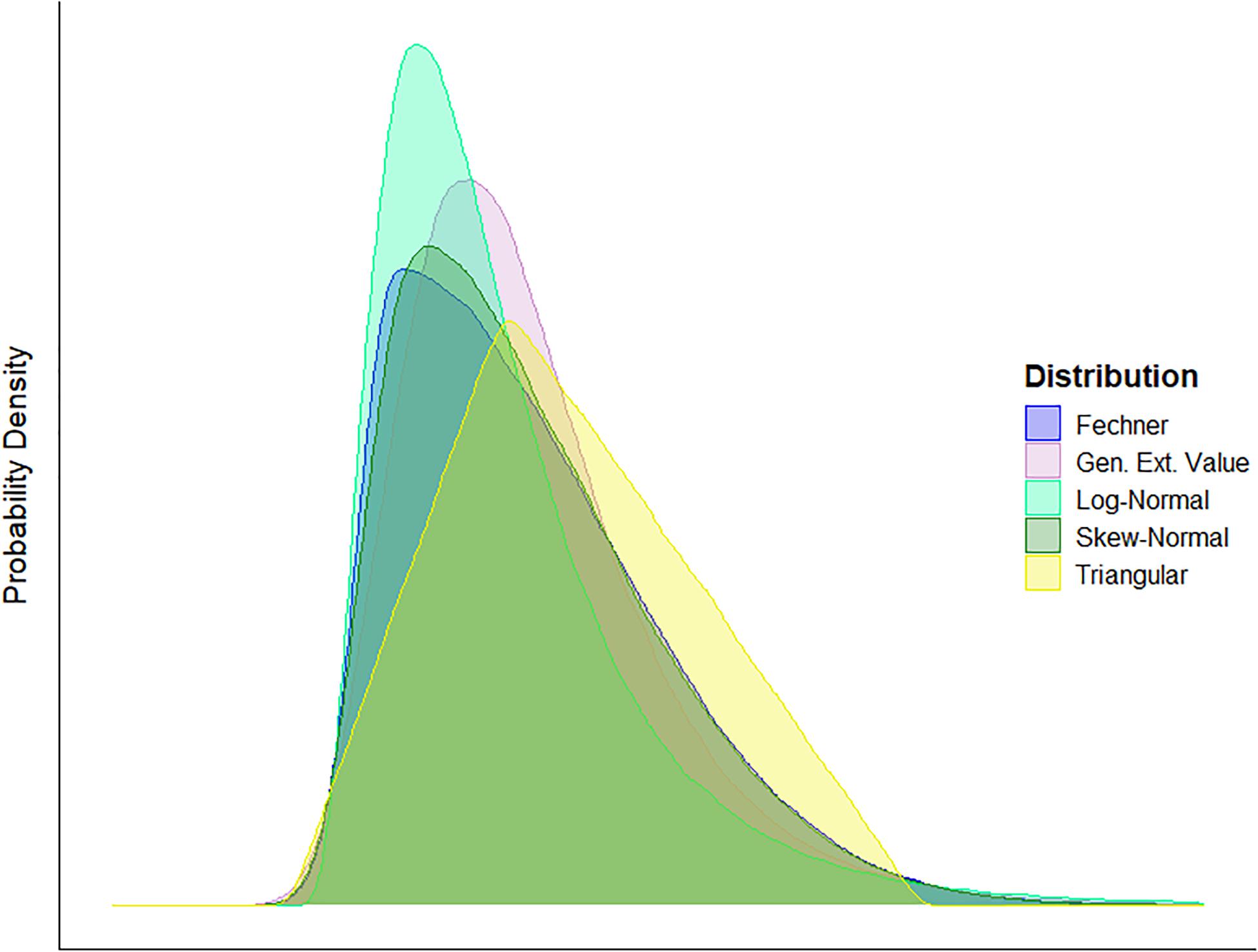
Figure 1. Comparison example of the probability distributions considered in the present study, fitted to a common emission factor.

These distributions were fitted to the official database of Costa Rican emission factors for the fuel sector (IMN, 2020). This database includes the accepted value for the emission factor f and two additional values U_R (also called “right uncertainty” or “upper uncertainty”, corresponding to the upper bound of the 95 % probability range estimated for the emission factor) and U_L (also called “left uncertainty” or “lower uncertainty,” corresponding to the lower bound of the 95 % probability range estimated for the emission factor) that delimit an asymmetric interval of possible values. Subsequently, this information was used to estimate the parameters of each distribution in order to calculate its theoretical variance (σ²) and its corresponding standard uncertainty $u_x=\sqrt{{\mathrm{\sigma }}^2}$. The standard uncertainty was also estimated and compared for each emission factor using method 1 of “symmetrization” proposed by Audi et al. (2017). The details of each distribution and the chosen symmetrization method are shown below. Except in cases where it is specified, the distribution mean μ was set to f.

Following the methodology proposed by Possolo et al. (2019), it was considered that each input f has an underlying asymmetric probability distribution qualified by U_R and U_L, both positives. However, according to IPCC good practices and guidelines (Intergovernmental Panel on Climate Change [IPCC], 2000, 2006), the interval [f-U_L, f+U_R] covers the true value of f with an approximate probability of 95 %. Also, it was assumed that “probabilities 0 < p_L < p_M < p_R < 1 are specified such that p_L = Pr{X < f−U_L}, p_M = Pr{X < f}, and p_R = Pr{X < f + U_R}, where X denotes the random variable modeling the uncertainty associated with f″ (Possolo et al., 2019). In all cases, p_L and p_R were set to 0.025 and 0.975, respectively. For the cases of Fechner, skew-normal and generalized extreme values, p_M was set to 0.50 and the applied methods sought to best reproduce f-U_L, f, and f+U_R as the specified percentiles of the corresponding distribution, using a non-linear, unweighted least-squares method.

Finally, to evaluate the fit of each distribution, populations of size 10⁶ were simulated with the estimated uncertainties or the distribution parameters that originated them. Since the present study focuses on uncertainty estimation, quantiles 2.5 % (q_2.5) and 97.5 % (q_97.5) were extracted from each generated population and compared with the original values of U_L and U_R included in the official database. The largest absolute relative error (RE) was reported as fitting statistic, according to Equation (3).

$RE=\max (\left|\frac{q_{2.5}-U_L}{U_L}\right|,\left|\frac{q_{97.5}-U_R}{U_R}\right|)(3)$

For all the calculations, data processing, statistical evaluation and simulations, the free environment for statistical computing R version 3.6.1 (R Core Team, 2020) was used. The programming code used in this study can be consulted in Supplementary Material.

Asymmetric Triangular Distribution (u_Tri)

As its name indicates, this distribution consists of a triangle whose maximum height is not in its center, and can be asymmetric to the left or to the right. The asymmetric triangular distribution consists of three parameters: the mode μ, the lower extreme value a, and the upper extreme value b. The variance of any triangular distribution is theoretically estimated by following Equation (4).

${\mathrm{\sigma }}^2=\frac{a^2+{\mathrm{\mu }}^2+b^2-a\mathrm{\mu }-b\mathrm{\mu }-ab}{18}(4)$

For the estimation of the parameters, the geometric estimation of the two-half triangles area was used (Petty and Dye, 2013). Considering μ=f, the equation system shown in (5) was obtained. This system was solved using Broyden and Newton methods (Dennis and Schnabel, 1996) included in the R-package nleqslv functions (Hasselman, 2018). For the population simulation, computational facilities provided by R-package triangle (Carnell, 2019) were used.

$\{\begin{array}{c}\hfill b-a-{\left(U_L-a\right)}^2/[0.025\left(f-a\right)]\hfill \\ \hfill b-a-{\left(b-U_R\right)}^2/[0.025\left(b-f\right)]\hfill \end{array}(5)$

Log-Normal Distribution (u_LN)

As its name indicates, the logarithmic normal distribution corresponds to the probability distribution of a variable whose natural logarithm results in a normal distribution. Its most common uses include modeling the multiplicative products of independent factors and strictly positive continuous variables with wide ranges (Intergovernmental Panel on Climate Change [IPCC], 2006). This distribution consists of two parameters: the mean μ and the variance σ², corresponding to the natural logarithm of the mean and variance of the normally distributed variable. According to the IPCC guidelines, it is possible to estimate the distribution variance σ² from uncertainties U_L, U_R and mean μ following Equation (6), where σ_g corresponds to the geometric standard deviation of the distribution, estimated according to Equation (7).

${\mathrm{\sigma }}^2={\mathrm{\mu }}^2\cdot e^{{\left(\ln {\mathrm{\sigma }}_g\right)}^2}-1(6)$

$-1.96\cdot \ln {\mathrm{\sigma }}_g=\frac{\left(\ln U_L+\ln U_R\right)}{2}(7)$

Finally, a correction factor F_C is recommended to slightly increase u as u_LNC=u_LN⋅F_C for cases with high standard uncertainties (u_rel > 50 %) (Intergovernmental Panel on Climate Change [IPCC], 2006; DCC and LCM, 2020). The estimation of the factor F_C is shown in Equation (8), adapted from Frey (2003) and Intergovernmental Panel on Climate Change [IPCC] (2006) considering the use of a standard uncertainty (u) instead of a half interval uncertainty (U), where u_rel=100⋅u_LN/f. Both u_LN and u_LNC were estimated and evaluated in the present study. For the simulation process, R-package stats functions were used (R Core Team, 2020).

$F_C={\left(\frac{-0.36+1.0921\cdot u_{rel}-0.00326\cdot u_{rel}^2+4.44\cdot {10}^{-5}\cdot u_{rel}^3}{u_{rel}}\right)}^2(8)$

Fechner Distribution (u_Fech)

Also known as split normal distribution (Wallis, 2014), this distribution “consists of two half-normal distributions with the same mode, one to the left of the mode, the other to the right of the mode, and with their respective densities suitably rescaled so that the resulting probability density is continuous” (Possolo et al., 2019). This distribution can be asymmetric to the left or to the right, depending on the magnitude of their respective parameters. The Fechner distribution consists of three parameters: the mode μ, the left variance ${\mathrm{\sigma }}_L^2$ and the right variance ${\mathrm{\sigma }}_R^2$. The Fechner distribution variance is theoretically estimated following Equation (9). A Fechner distribution may be a suitable model if 0.410 < U_R/U_L < 2.44 for a coverage probability of 95 % (Possolo et al., 2019).

${\mathrm{\sigma }}^2=\left(1-\frac{2}{\mathrm{\pi }}\right){\left({\mathrm{\sigma }}_R-{\mathrm{\sigma }}_L\right)}^2+{\mathrm{\sigma }}_R{\mathrm{\sigma }}_L(9)$

For the estimation of the parameters and the simulation process, the code already generated by Possolo et al. (2019) was used, which uses the computational facilities of R-package fanplot (Abel, 2015).

Skew-Normal Distribution (u_SN)

This distribution is a generalization of the Gaussian (normal) distribution that considers an additional bias parameter (α). This bias allows this distribution for asymmetry to the left or right, depending on the value of α (for the traditional Gaussian distribution, α= 0). The skew-normal distribution consists of three parameters: a location parameter μ, a scale parameter ω > 0, and the bias parameter α (Azzalini and Capitanio, 2014). The skew-normal distribution variance is theoretically estimated by following Equation (10). A skew-normal distribution may be a suitable model if 0.410 < U_R/U_L < 2.44 for a coverage probability of 95 % (Possolo et al., 2019).

${\mathrm{\sigma }}^2={\mathrm{\omega }}^2\left[1-\frac{2{\mathrm{\alpha }}^2}{\mathrm{\pi }\left(1+{\mathrm{\alpha }}^2\right)}\right](10)$

For the estimation of the parameters and the simulation process, the code already generated by Possolo et al. (2019) was used, which uses the computational facilities of R-package sn (Azzalini, 2020).

Generalized Extreme Value Distribution (u_GEV)

The extreme value distributions are generally considered to comprise three distribution families, including the Gumbel, Fréchet, Gompertz, and reverse Weibull distributions (Possolo et al., 2019). These distributions may all be represented as members of a single family of generalized distributions with a common cumulative distribution function, known as the generalized extreme value distribution (GEVD). The GEVD consists of three parameters: a location parameter μ, a scale parameter ω > 0, and a shape parameter ξ (Johnson et al., 1995). The GEVD variance is theoretically estimated by following Equation (11),

${\mathrm{\sigma }}^2=\left(g_2-g_1^2\right)\frac{{\mathrm{\omega }}^2}{{\xi }^2}(11)$

where g_k = Γ(1−kξ) and Γ is the gamma function. For the estimation of the parameters and the simulation process, the code already generated by Possolo et al. (2019) was used, which uses the computational facilities of R-package evd (Stephenson, 2002).

Symmetrization Method (u_Sym)

This method consists of a simple approximation of an asymmetric distribution as a “symmetric” normal distribution. Audi et al. (2017) mention it as method 1 and only requires estimating the difference between U_R and U_L. The resulting value is considered equivalent to the coverage interval (with the same coverage probability as interval [f-U_L, f+U_R]) for a normal distribution centered at μ=(U_R+U_L)/2. Considering the properties of the normal distribution, it is possible to obtain the relationship shown in Equation (12), where σ is the standard deviation for the “symmetrized” distribution. For the simulation process, R-package stats functions were used (R Core Team, 2020).

$\mathrm{\sigma }=\frac{U_L-U_R}{4}(12)$

Results and Discussion

Figure 2 shows an example of the obtained results for each of the asymmetric distributions and the symmetrization method applied to a single source: lubricant (for commercial, institutional, residential, agricultural and land transportation use). This specific source was selected because its results are highly representative of the general behavior observed in the other sources and factors. Rows on the figure represent the three emission factors (CO₂, CH₄, and N₂O) included in the official Costa Rican database for most sources, including lubricant. Upper side of the figure illustrates the simulated distributions behavior and lower side of the figure compares the estimated intervals defined by quantiles 2.5 % (q_2.5) and 97.5 % (q_97.5) of the simulated populations with the [f-U_L, f+U_R] reference interval as a visual aid to interpret the RE values.

FIGURE 2

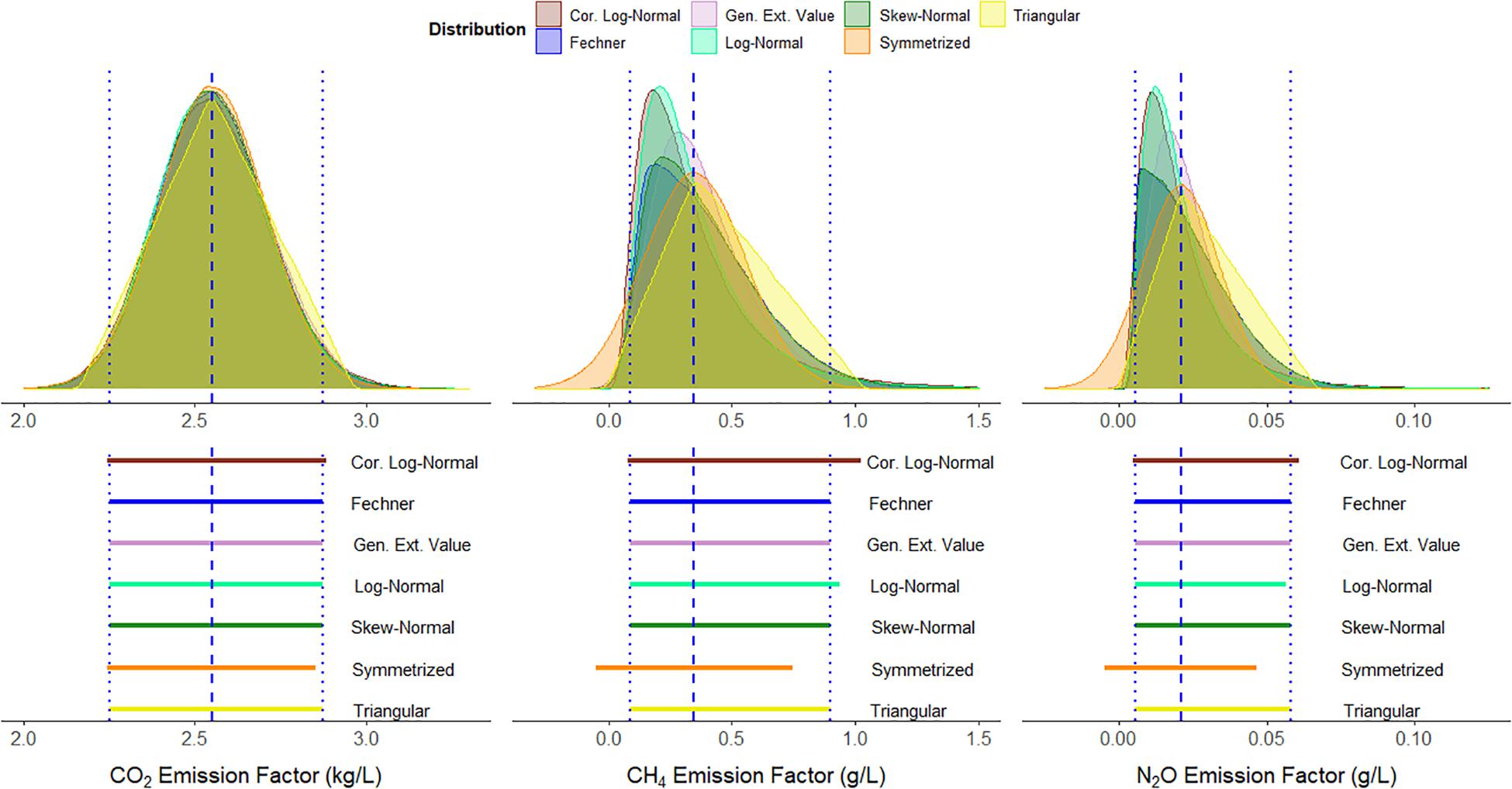
Figure 2. Comparison of various distributions fitted to the emission factors for CO₂, CH₄, and N₂O in lubricant (for commercial, institutional, residential, agricultural and land transportation use) and their corresponding intervals covering 95 % of the simulated population for each distribution. The left column of figures corresponds to results for CO₂ emission factor, with the fitted distributions on the upper side and 95 % intervals on the lower side. The middle column of figures corresponds to CH₄ emission factor and the right column of figures to N₂O emission factor, with fitted distributions on the upper side and 95 % intervals on the lower side. The dashed line corresponds to the best estimate reported f and the dotted lines to its asymmetric interval [f-U_L, f+ U_R] covering an approximate probability of 95 % taken from the official database of Costa Rican emission factors (IMN, 2020).

Tables 1–3 show the complete results for each of the asymmetric distributions and the symmetrization method applied to all the official Costa Rican emission factors for the fuel sector. These results correspond to the estimated standard uncertainties (u) and the maximum relative errors obtained for the quantiles of interest (RE) after the respective simulations and intervals estimation. All estimated standard uncertainties are reported as absolute uncertainties. However, due to their widespread use in the GHG sector, the corresponding relative standard uncertainties are shown in Supplementary Tables 1–3.

TABLE 1

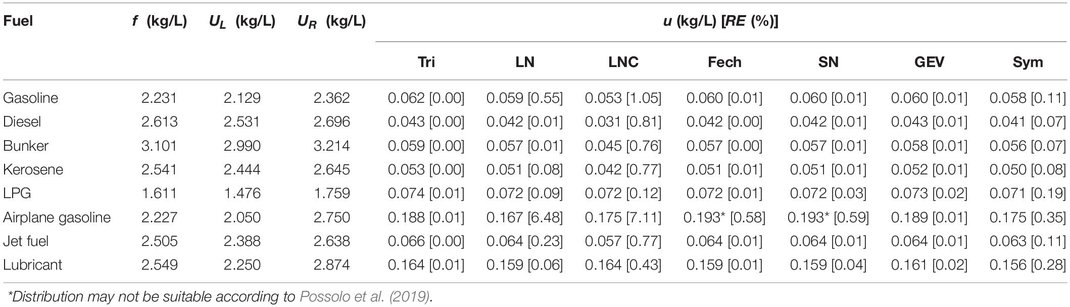
Table 1. Absolute standard uncertainties u and largest relative error RE estimated for CO₂ emission factors for the fuel sector using various asymmetric approaches. The best estimate f and expanded asymmetric uncertainties U_L and U_R were taken from the official database of Costa Rican emission factors (IMN, 2020). Values of RE are shown inside the brackets.

Table 1 and Supplementary Table 1 show the results corresponding to the CO₂ emission factors (left column of Figure 2 as example). These factors have the particularity of reporting the least asymmetric intervals of all the analyzed database. All distributions have standard uncertainty values similar to each other, except for the corrected log-normal distribution. This behavior was expected since correction factor F_C is only recommended for cases with high standard uncertainties. The asymmetric triangular distribution systematically showed the largest standard uncertainties, while the smallest standard uncertainties were evidenced with the corrected log-normal distribution or the symmetrization method. The greatest differences between the standard uncertainties were evidenced in the emission factor for airplane gasoline, corresponding to the most asymmetric interval in the tables. It should be noted that the uncertainties estimated for this factor with Fechner (u_Fech) and skew-normal (u_SN) distributions may not be suitable for the interval asymmetry, due to the non-compliance of the recommendation 0.410 < U_R/U_L < 2.44 in both cases according to Possolo et al. (2019).

When evaluating the distribution fitting in Table 1 and Supplementary Table 1 through RE values for the simulated populations, it is noted that the best fitting is obtained for the asymmetric triangular and GEV distributions with RE < 0.03 in all cases. Subsequently, the Fechner and skew-normal distributions showed RE < 0.05 in all cases except for the airplane gasoline factor mentioned above (RE_Fech = 0.58, RE_SN = 0.59). The symmetrization method and the log-normal distribution showed similar fittings, with a slight improvement for the first (RE_Sym ≤ 0.35). Finally, the corrected log-normal distribution did not show to be useful for such small asymmetries and small relative uncertainty values as expected (RE_LNC ≤ 7.11).

Table 2 and Supplementary Table 2 show the results corresponding to the CH₄ emission factors (middle column of Figure 2 as example) while Table 3 and Supplementary Table 3 do the same for N₂O emission factors (right column of Figure 2 as example). The factors for both gases showed percentage variation intervals with asymmetries greater than the CO₂ factors and similar to each other. The corrected log-normal distribution systematically showed the largest standard uncertainties (except for one case in N₂O), while the smallest standard uncertainties were evidenced for the log-normal distribution or the symmetrization method. However, the results obtained for the symmetrization method should be taken with caution. Given the characteristics of the normal distribution assumed by this method and the proximity of the intervals to 0, the simulated populations presented a significant percentage of negative values (between 5 % and 10 %), which contradict the physical nature of an emission factor. The asymmetric triangular, Fechner, skew-normal, and GEV distributions shared the possibility to theoretically present negative results, but the proportions of values below 0 obtained in the simulated populations were considered insignificant (<0.2 %). For this reason, only the use of this symmetrization method is not recommended for the evaluated CH₄ and N₂O emission factors.

TABLE 2

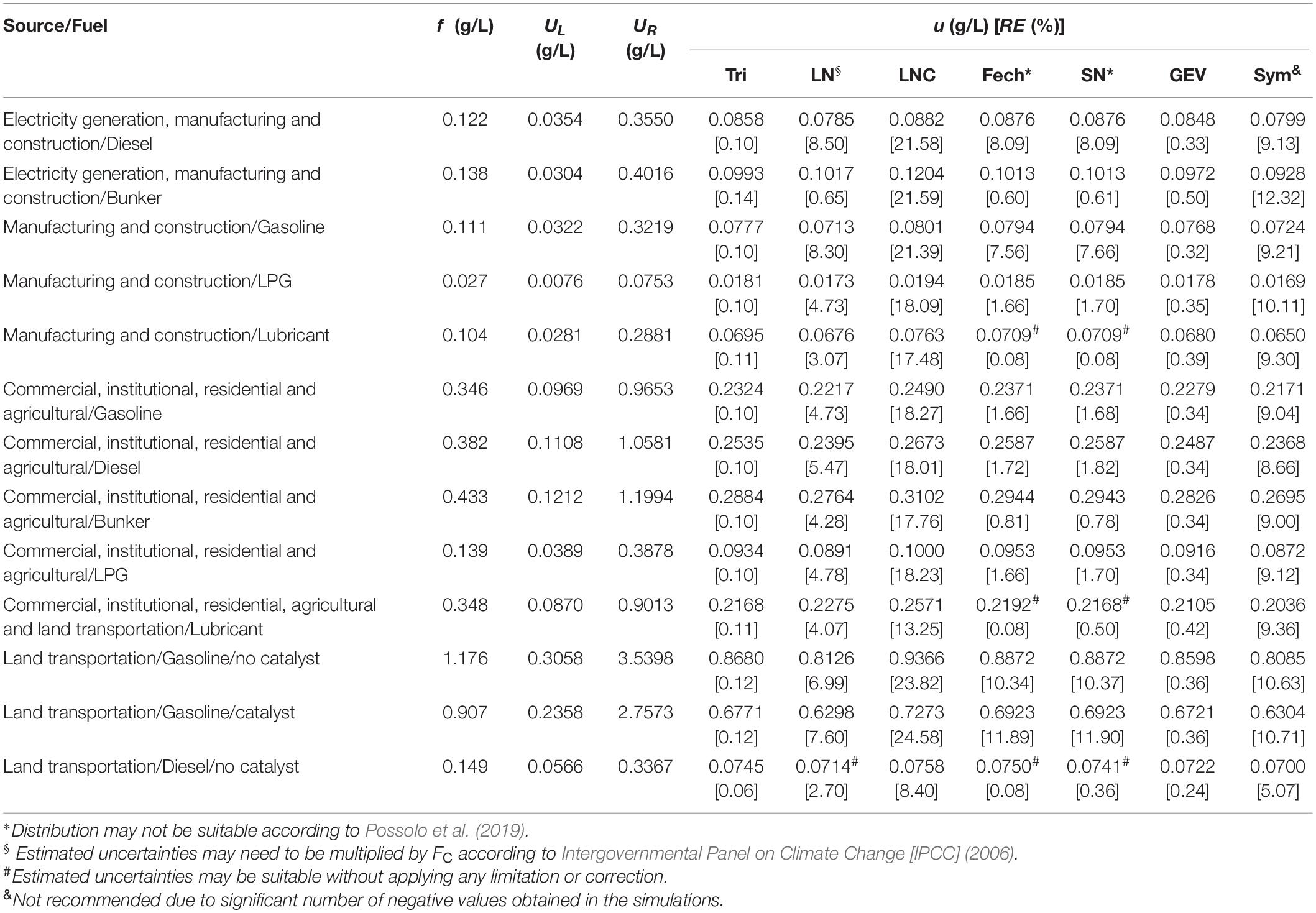
Table 2. Absolute standard uncertainties u and largest relative error RE estimated for CH₄ emission factors for the fuel sector using various asymmetric approaches. The best estimate f and expanded asymmetric uncertainties U_L and U_R were taken from the official database of Costa Rican emission factors (IMN, 2020). Values of RE are shown inside the brackets.

TABLE 3

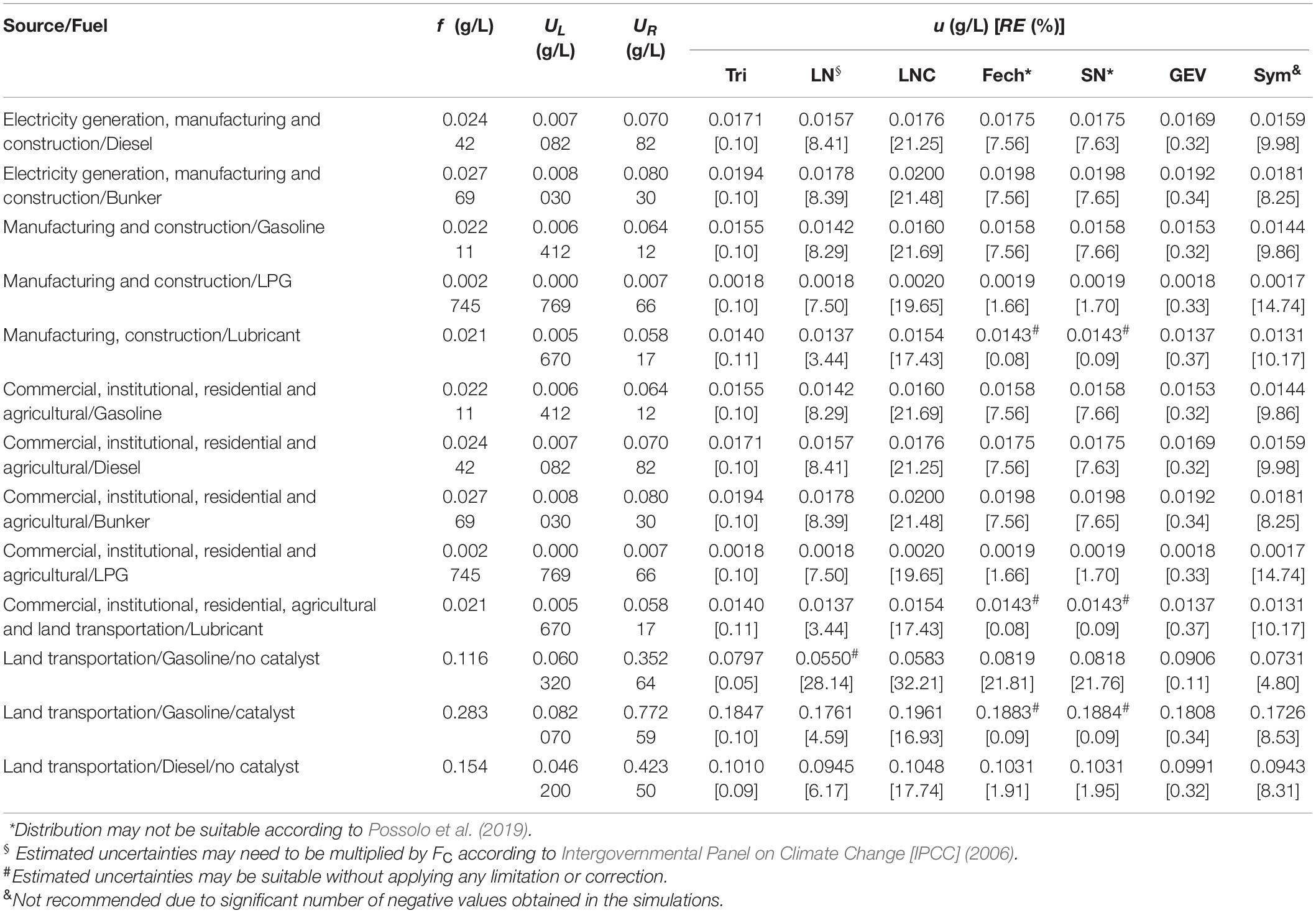
Table 3. Absolute standard uncertainties u and largest relative error RE estimated for N₂O emission factors for the fuel sector using various asymmetric approaches. The best estimate f and expanded asymmetric uncertainties U_L and U_R were taken from the official database of Costa Rican emission factors (IMN, 2020). Values of RE are shown inside the brackets.

The greatest differences between standard uncertainties for the CH₄ emission factors were evidenced for lubricants due to the little similarity between the corrected log-normal distribution and the other distributions. It should be noted that these cases do not correspond to the factor with the greatest asymmetry in Table 2 and Supplementary Table 2, as occurred with the CO₂ emission factors. For the N₂O emission factors, the greatest differences were evidenced for the gasoline without catalyst in land transportation factor. This factor does correspond to the most asymmetric interval in Table 3 and Supplementary Table 3, with reduced values for both log-normal methods while the highest value was evidenced in the GEV distribution (the only emission factor with this behavior).

It should be noted again that most of u_Fech and u_SN may not be suitable for the emission factor asymmetries of both gases due to non-compliance with recommendation 0.410 < U_R/U_L < 2.44 (Possolo et al., 2019). Compliance with this criterion was only evidenced for five CH₄ emission factors and five N₂O emission factors. Uncertainties estimated with the log-normal distribution u_LN should also be highlighted. According to the IPCC guidelines (Intergovernmental Panel on Climate Change [IPCC], 2006), these uncertainties could be underestimated due to their high percentage values relative to the emission factor (u_rel > 50 %). Therefore, it would be initially recommended to use u_LNC instead.

When evaluating the distribution fitting in the factors of both gases through RE values for the simulated populations, it is again noted that the best fitting is obtained for the asymmetric triangular distribution (RE_Tri < 0.2) and GEV distribution (RE_GEV ≤ 0.5), respectively. The case of N₂O emission factor for gasoline without catalyst in land transportation should be highlighted, where these methods seem to fit adequately (RE_Tri = 0.05, RE_GEV = 0.11), but their relative standard uncertainties differ by more than 9 % (u_Tri = 68.71 %, u_GEV = 78.10 %). This situation does not occur in any other emission factor for CO₂, CH₄, or N₂O, where RE values and standard uncertainties between both distributions seem to be consistent with each other. For Fechner and skew-normal distributions, the ten emission factors in which their use may be appropriate showed very good fittings as well (RE_Fech < 0.1, RE_SN ≤ 0.5), while mixed fittings were evidenced for the other factors (0.6 < RE < 21.9) and for the log-normal distribution (0.6 < RE_LN < 28.2). Although not recommended, the symmetrization method was not very effective when evaluating its fitting in these emission factors (4.8 < RE_Sym < 14.8). It is noteworthy that, according to the IPCC guidelines (Intergovernmental Panel on Climate Change [IPCC], 2006), the high uncertainties would justify the use of the correction factor F_C to improve the estimation of the log-normal distribution. However, the corrected log-normal distribution fittings were the worst for all factors for both gases (8.4 < RE_LNC < 32.3). In this context, a deeper analysis is recommended on the use of Equation (8) adaptation for the correction of standard uncertainties from a log-normal distribution instead of the original equation stated on Frey (2003) and Intergovernmental Panel on Climate Change [IPCC] (2006) for half interval uncertainties.

Although most of the proposed methods can be used to estimate the standard uncertainties of the emission factors included in the official Costa Rican database for the fuel sector (except for symmetrization method for CH₄ and N₂O emission factors), the asymmetric triangular and GEV distributions obtained the best fittings in the present study. For practical purposes, any of these two distributions could be chosen to estimate the standard uncertainty for Costa Rican fuel emission factors, with little difference in the results in most cases. Its use can also be recommended to address the estimation of standard uncertainties for other emission factors, even for other countries, as long as the probability of obtaining negative values is not a concern (for example, emission factors with U_L values close to 0). In the latter cases, the use of a log-normal distribution is recommended or exploring the use of truncated variants of the distributions evaluated in the present study that prevent the presence of negative values.

Conclusion

From the present study, the applicability of different approaches of asymmetric distributions to address standard uncertainty estimation of emission factors in GHG inventories according to GUM guidelines was evident, specifically for the Costa Rican official database of these factors in the fuel sector. The comparability of the different methods applied was also appreciable, with significant differences in the fittings obtained for factors with probability ranges or coverage intervals reported with greater asymmetries. Overall, a systematically better fit was evidenced for the asymmetric triangular and generalized extreme value distributions, both for CO₂ emission factors with less asymmetries and CH₄ and N₂O emission factors with greater asymmetries. The observed fit was not as good for the other distributions, with the log-normal distribution applying the correction factor suggested in the literature showed the worst results.

Therefore, the use of the asymmetric triangular or generalized extreme value distributions is recommended indistinctly to estimate the standard uncertainties associated with the emission factors from the official Costa Rican database for the fuel sector. Its use is also recommended within the process of implementing uncertainty estimation in GHG inventories and improving the quality of its results, considering other emission factors for Costa Rica or other countries as well, provided that their intervals of variation are not very close to 0. Further, depending on the total emissions inventory characteristics (e.g., expected asymmetry), the probability distributions addressed in this study can be considered for the total uncertainty of the inventory, broadening the spectrum of possibilities already used.

Finally, it is considered that the present study provides the expected guidance for the interpretation and manipulation of emission factor standard uncertainties and will hopefully ease the process of implementing uncertainty estimation in GHG inventories and obtain a more precise and reliable quantification of emission data from the fossil-fueled transportation sector in Costa Rica and other countries around the world.

Data Availability Statement

The original contributions presented in the study are included in the article/Supplementary Material, further inquiries can be directed to the corresponding author/s.

Author Contributions

GM-C contributed to the conception of the study, performed the statistical analysis, and wrote the first draft of the manuscript. BC-J revised it critically for important intellectual content and approved for publication of the content. Both authors contributed to the article and approved the submitted version.

Funding

The publication of this study was covered by the NDC Support Programme of the United Nations Development Programme (UNDP).

Conflict of Interest

The authors declare that the research was conducted in the absence of any commercial or financial relationships that could be construed as a potential conflict of interest.

Acknowledgments

We would like to thank Dr. Antonio Possolo (Statistical Engineering Division, National Institute of Standards and Technology, NIST) for his valuable guidance on the topic and general review of the manuscript. We also wish to thank Dr. Gilbert Brenes-Camacho (School of Statistics, Costa Rican University, UCR) for his technical review of the manuscript.

Supplementary Material

The Supplementary Material for this article can be found online at: https://www.frontiersin.org/articles/10.3389/fenvs.2021.662052/full#supplementary-material

References

Abel, G. (2015). fanplot: an R package for visualizing sequential distributions. R J. 7, 15–23. doi: 10.32614/RJ-2015-002

CrossRef Full Text | Google Scholar

Allen, K., and Padgett-Vásquez, S. (2017). Forest cover, development, and sustainability in Costa Rica: can one policy fit all? Land Use Policy 67, 212–221. doi: 10.1016/j.landusepol.2017.05.008

CrossRef Full Text | Google Scholar

Audi, G., Kondev, F. G., Wang, M., Huang, W. J., and Naimi, S. (2017). The Nubase2016 evaluation of nuclear properties. Chin. Phys. C. 41:030001. doi: 10.1088/1674-1137/41/3/030001

CrossRef Full Text | Google Scholar

Azzalini, A. (2020). The Skew-Normal and Related Distributions Such as the Skew-t [version 1.6-2]. Available online at: http://azzalini.stat.unipd.it/SN (Accessed 21, Oct 2020)

Google Scholar

Azzalini, A., and Capitanio, A. (2014). The Skew-Normal and Related Families. Cambridge: Cambridge University Press.

Google Scholar

Barlow, R. (2004). Asymmetrical Statistical Errors. Available online at: https://arxiv.org/abs/physics/0406120 (Accessed 21 Oct 2020).

Google Scholar

Bharvirkar, R. (1999). Quantification of Variability and Uncertainty in Emission Factors and Emissions Inventories. Master’s thesis, North Carolina State University, Raleigh, NC.

Google Scholar

Carnell, R. (2019). Triangle: Provides the Standard Distribution Functions for the Triangle Distribution [Version 0.12]. Available online at: https://bertcarnell.github.io/triangle/ (Accessed 17 Oct 2020).

Google Scholar

Choulga, M., Janssens-Maenhout, G., Super, I., Agusti-Panareda, A., Balsamo, G., Bousserez, N., et al. (2020). Global Anthropogenic CO2 Emissions and Uncertainties as Prior for Earth System Modelling and Data Assimilation. Available online at: https://doi.org/10.5194/essd-2020-68 (Accessed 11 Mar 2021).

Google Scholar

Courvisanos, J., and Ameeta, J. (2006). A framework for sustainable Ecotourism: application to Costa Rica. Tour. Hosp. Plan. Dev. 3, 131–142. doi: 10.1080/14790530600938378

CrossRef Full Text | Google Scholar

DCC and LCM (2020). Guía Metodológica para la Estimación y análisis de la Incertidumbre de Emisiones y Remociones de gases de Efecto Invernadero (GEI). National Carbon Neutrality PROGRAM 2.0. Available online at: https://cambioclimatico.go.cr/wp-content/uploads/2020/11/PPCN-GuiaIncertidumbre.pdf (Accessed 23 Nov 2020).

Google Scholar

DCC and PMR (2020). Programa País de Carbono Neutralidad: Categoría Organizacional. National Carbon Neutrality Program 2.0. Available online at: https://cambioclimatico.go.cr//wp-content/uploads/2020/04/1-PPCN_Organizacional.pdf (Accessed 10 Oct 2020)

Google Scholar

Dennis, J. E., and Schnabel, R. B. (1996). Numerical Methods for Unconstrained Optimization and Nonlinear Equations. Philadelphia, PA: SIAM.

Google Scholar

EPA (1996). Evaluating the uncertainty of emission estimates. Final Report. Emission Inventory Improvement Program. Available online at: https://www.epa.gov/sites/production/files/2015-08/documents/vi04.pdf (Accesed 05 Oct 2020).

Google Scholar

EPA (2002). Quality Assurance / Quality Control and Uncertainty Management Plan for the US Greenhouse Gas inventory: Procedures Manual for Quality Assurance / Quality Control and Uncertainty Analysis. Available online at: https://nepis.epa.gov/Exe/ZyPURL.cgi?Dockey=P1005GXH.TXT (Accessed 05 Oct 2020).

Google Scholar

Fendt, L. (2017). All that Glitters is not Green: Costa Rica’s Renewables Conceal Dependence on Oil. Available online at: https://www.theguardian.com/world/2017/jan/05/costa-rica-renewable-energy-oil-cars (Accessed 26 Jan 2021).

Google Scholar

Frey, C. (2003). Evaluation of an Approximate Analytical Procedure for Calculating Uncertainty in the Greenhouse Gas Version of the Multi-Scale Motor Vehicle and Equipment Emissions System. Ann Arbor, MI: U.S. Environmental Protection Agency.

Google Scholar

Frey, C. (2007). Quantification of Uncertainty in Emission Factors and Inventories. Emission Inventory Conference, NC. Available online at: https://www3.epa.gov/ttnchie1/conference/ei16/session5/frey.pdf (Accessed 06 Oct 2020).

Google Scholar

Government of Costa Rica (2019). National Decarbonization Plan (Plan Nacional de Descarbonización). Available online at: https://cambioclimatico.go.cr/wp-content/uploads/2019/02/PLAN.pdf (Accessed 26 Jan 2021).

Google Scholar

Hasselman, B. (2018). nleqslv: Solve Systems of Nonlinear Equations [version 3.3.2]. Available online at: https://CRAN.R-project.org/package=nleqslv (Accessed 20 Oct 2020).

Google Scholar

ICE Group (2020). We Are Renewable and Solidary Energy. Available online at: https://www.grupoice.com/wps/wcm/connect/579dfc1f-5156-41e0-807d-d6808f65d718/Fasciculo_Electricidad_2020_ingl%C3%A9s_compressed.pdf?MOD=AJPERES&CVID=m.pGzcp (Accessed 26 Jan 2021).

Google Scholar

IMN (2020). Factores de Emisión de Gases de efecto Invernadero, 10th Edn. National Meteorology Institute of Costa Rica. Available online at: http://cglobal.imn.ac.cr/index.php/publications/factores-de-emision-gei-decima-edicion-2020/ (Accessed 16 Oct 2020).

Google Scholar

Intergovernmental Panel on Climate Change [IPCC] (2000). Good Practice Guidance and Uncertainty Management in National Greenhouse Gas Inventories. Quantifying Uncertainties in Practice. Intergovernmental Panel on Climate Change, Methodology Report for the National Greenhouse Gas Inventories Programme. Available online at: https://www.ipcc.ch/publication/good-practice-guidance-and-uncertainty-management-in-national-greenhouse-gas-inventories/ (Accessed 01 Oct 2020).

Google Scholar

Intergovernmental Panel on Climate Change [IPCC] (2006). Volume 1: General Guidance and Reporting – Uncertainties. 2006 IPCC Guidelines for National Greenhouse Gas Inventories. Available online at: https://www.ipcc-nggip.iges.or.jp/public/2006gl/vol1.html (Accessed 01 Oct 2020).

Google Scholar

ISO 14064-1. (2006). Greenhouse Gases — Part 1: Specification with Guidance at the Organization Level for Quantification and Reporting of Greenhouse gas Emissions and Removals. Geneva: International Organization for Standardization.

Google Scholar

ISO 14064-1. (2018). Greenhouse Gases — Part 1: Specification with Guidance at the Organization Level for Quantification and Reporting of Greenhouse Gas Emissions and Removals. Geneva: International Organization for Standardization.

Google Scholar

Joint Committee for Guides in Metrology [JCGM] (2008). Evaluation of Measurement Data – Guide to the Expression of Uncertainty in Measurement GUM: 1995 with minor corrections. Joint Committee for Guides in Metrology, JCGM:100. Available online at: http://www.bipm.org/utils/common/documents/jcgm/JCGM_100_2008_E.pdf. (Accessed 01 Nov 2020).

Google Scholar

Joint Committee for Guides in Metrology [JCGM] (2012). International Vocabulary of Metrology – Basic and general concepts and associated terms (VIM): 2008 with minor corrections. Joint Committee for Guides in Metrology, JCGM:200. Available online at: https://www.bipm.org/utils/common/documents/jcgm/JCGM_200_2012.pdf. (Accessed 08 Mar 2021).

Google Scholar

Johnson, N., Kotz, S., and Balakrishnan, N. (1995). Continuous Univariate Distributions, 2nd Edn, Vol. 2. New York, NY: John Wiley & Sons Inc.

Google Scholar

Jonas, M., White, T., Marland, G., Lieberman, D., Nahorski, Z., and Nilsson, S. (2010). “Dealing with uncertainty in GHG inventories: how to go about it?,” in Coping with Uncertainty. Lecture Notes in Economics and Mathematical Systems, Vol. 633, eds K. Marti, Y. Ermoliev, and M. Makowski 229–245. doi: 10.1007/978-3-642-03735-1_11

CrossRef Full Text | Google Scholar

Milne, A., Glendining, M., Lark, R. M., Perryman, S., Gordon, T., and Whitmore, A. (2015). Communicating the uncertainty in estimated greenhouse gas emissions from agriculture. J. Environ. Manag. 160, 139–153. doi: 10.1016/j.jenvman.2015.05.034

PubMed Abstract | CrossRef Full Text | Google Scholar

Petty, N. W., and Dye, S. (2013). Notes on Triangular Distributions. Statistics Learning Centre. Available online at: https://learnandteachstatistics.files.wordpress.com/2013/07/notes-on-triangle-distributions.pdf (Accessed 18 Oct 2020).

Google Scholar

Possolo, A., and Iyer, H. (2017). Concepts and tools for the evaluation of measurement uncertainty. Rev. Sci. Instrum. 88:011301. doi: 10.1063/1.4974274

CrossRef Full Text | Google Scholar

Possolo, A., Merkatas, C., and Bodnar, O. (2019). Asymmetrical uncertainties. Metrologia 56:045009. doi: 10.1088/1681-7575/ab2a8d

CrossRef Full Text | Google Scholar

R Core Team (2020). R: A language and Environment for Statistical Computing [version 3.6.3]. Vienna: R Foundation for Statistical Computing.

Google Scholar

Ritter, K., Lev-On, M., and Shires, T. (2010). Understanding uncertainty in greenhouse gas emission estimates: Technical considerations and statistical calculation methods. Paper Presented at the 19th Annual International Emission Inventory Conference, Texas.

Google Scholar

Rypdal, K., and Winiwater, W. (2001). Uncertainties in greenhouse gas emission inventories – evaluation, comparability and implications. Environ. Sci. Policy 4, 107–116. doi: 10.1016/S1462-9011(00)00113-1

CrossRef Full Text | Google Scholar

Solazzo, E., Crippa, M., Guizzardi, D., Muntean, M., Choulga, M., and Janssens-Maenhout, G. (2020). Uncertainties in the EDGAR Emission Inventory of Greenhouse Gases. Available online at: https://doi.org/10.5194/acp-2020-1102 (Accessed 11 Mar 2021).

Google Scholar

Stephenson, A. G. (2002). evd: extreme value distributions. R News 2, 31–32.

Google Scholar

UN Environment Programme (2019). Costa Rica - Policy Leadership Award. Available online at: https://www.unenvironment.org/championsofearth/laureates/2019/costa-rica (Accessed 26 Jan 2021).

Google Scholar

Wallis, K. (2014). The two-piece normal, binormal, or double Gaussian distribution: its origin and rediscoveries. Statist. Sci. 29, 106–112. doi: 10.1214/13-STS417

CrossRef Full Text | Google Scholar