Abstract
With over 200,000 km2 of natural savannas, the Orinoquia region of Colombia is a key and strategic conservation area. Because of Colombia’s fast economic growth, there are significant plans for agro-industrial expansion in the Orinoquia. This expansion may seriously affect water availability. To evaluate the cumulative impacts on freshwater ecosystems derived by different expansion scenarios, the use of a comprehensive framework for mathematical modeling, able to represent the hydrological processes at a macro-basin scale, is crucial for analysis and as a tool to bridge the gap between science and practice. In this work, we developed a general methodological framework for hydrological analysis at macro-basin scale consisting of four main stages: 1) collection and processing of hydro-climatological data, 2) characterization of hydro dependent water use sectors, 3) mathematical modeling and 4) scenario simulation. As a result of applying the proposed framework, we obtained a coupled hydrological model, which allows us to represent the rain-runoff process, the river-floodplain interaction and anthropic processes such as surface water extraction and groundwater extraction, enabling us to represent the complexity of the Orinoquia region. The model was successfully implemented in Matlab showing a Nash-Sutcliffe efficiency coefficient between 0.62 and 0.92 in calibration and between 0.49 and 0.92 in validation. With this model we analyzed five different agro-industrial expansion scenarios, finding that the Colombian Orinoquia may have future high pressure on water resource areas with critical changes in the water availability regime. The scenarios show reductions of up to 85% in low water flows in more than 50% of the area of the Colombian Orinoco basin. In the most extreme scenarios, the Meta, Vichada and Guaviare rivers show reductions of 95, 98 and 50% in low water flows. The results show an urgent need to consider hydrology in planning processes to ensure the sustainability of this important area in Colombia.
Introduction
Traditionally, extensive cattle ranching has played an important role in the economy of the Colombian Orinoco (Andrade and Castro, 2012; Buriticá, 2016). However, in the last 2 decades, agriculture has expanded, reaching a significant increase from 1,000 km2 to 8,000 km2 of planted area (around 2.3% of the Colombian Orinoco basin). This expansion of the agricultural Frontier (Vargas et al., 2015; Cárdenas-Santamaría et al., 2018) may have a strong impact in savanna ecosystems, derived from the alteration of the land for crops such as rice, sugar cane and oil palm (Andrade and Castro, 2012). At the same time, it has led to an increase in water consumption for the different crops, generating substantial pressure on the water resources of this region.
The National Planning Department of Colombia (DNP, 2018) estimated that more than 150,000 km2 of the Colombian Orinoquia is suitable for agriculture, suggesting greater pressure on the water resources of this region in the future. Globally, agriculture consumes 70% of the global freshwater withdrawals due to crop evapotranspiration (FAO, 2017). Similarly, a large increase in crop area in the Orinoquia region would certainly affect water quantity and quality. Research has clearly established how agricultural expansion can have severe consequences for ecosystems (Byard, 1999; Kanianska, 2016; Rabin et al., 2020; Tamaris et al., 2017). The Colombian Orinoquia covers 8.5% of the flooded savannas in South America and it is a strategic ecosystem of great economic, biological and ecological importance for the country (Mora et al., 2015). It is also one of the most important biodiversity reserves in the neotropics (Gassón, 2002).
Adequate planning of the territory must be based on multiscale analysis, supported by measurements and mathematical modeling tools. These tools allow for prospective analysis and evaluation of the impacts on the territory in the face of future interventions. In Colombia, historically, most of the hydrological modeling efforts have focused on the Magdalena-Cauca basin, considered the most important basin in the country (Angarita et al., 2018; Craven et al., 2017; Labrador Cadena et al., 2016; Rodríguez et al., 2020). However, the Orinoquia region has been identified as the next major area of agro-industrial expansion in Colombia, so it is urgent to develop tools for prospective analysis. Considering this need, this study presents a hydrological modeling exercise with monthly time step for the Colombian Orinoquia region, addressed by two parsimonious conceptual models: the ABCD model proposed by Thomas (1981) and the river-floodplain interaction model proposed by Angarita et al. (2018). We developed a logical technical framework allowing for the description and understanding of the territory that, in a practical way, enables the evaluation of possible future scenarios and their impacts on water availability.
Study Area
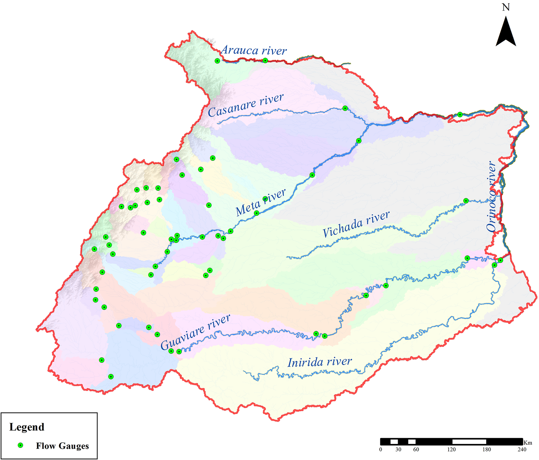
The Colombian Orinoquia region (Figure 1) has an area of 347,208 km2 covering the departments of Arauca, Casanare, Vichada, Guainía, Cundinamarca, Boyacá, Norte de Santander, Vaupés, Meta, Guaviare and Santander; it represents about 34% of the Colombian territory. It exhibits a unimodal pattern in the temporal distribution of precipitation in the annual cycle, with an average of 2,650 mm yr−1, which is largely associated with the greater convective activity generated by the southern migration of the Intertropical Convergence Zone (Poveda et al., 1998; Poveda and Mesa, 1996; Poveda and Rojas, 1997; Poveda et al., 2002; J. Velez et al., 2000). Temperature can vary between 23°C and 29°C during the year. Geologically, it consists of tertiary sedimentary rocks, which cover crystalline Precambrian rocks and sediments of the Paleozoic and Cretaceous (SGC, 2020). It also has a large variety of geomorphological structures that allow for the presence of a very diverse and complex drainage system, ranging from meandering to braided rivers. Thanks to the low slopes of its plain areas, the broad transversal sections of the channels (around 0.5–2 km) and the constant presence of land depressions around the rivers, there are bidirectional interactions between rivers and their savanna areas, generating large floods. Consistent with the rainfall regime, river flows are highest in June, July and August. The main tributaries that are part of the Orinoco basin in Colombia are the Meta river with a multi-year annual average flow of 4,973 m3 s−1, the Guaviare river with 4,035 m3 s−1, the Inírida river with 2,978 m3 s−1 and the Vichada river with 1,030 m3 s−1. In total, the Orinoco basin in Colombia provides 26.4% of the fresh water of the Colombian territory (IDEAM, 2019).
FIGURE 1

Location of the Orinoco basin in Colombia. The watershed boundary is delimited by the red line. Flooded savannas are shown in light blue.
Methodology
The study of water systems implies knowing their character, behavior, distribution and condition (Brierley and Fryirs, 2004). Therefore, for this study we have conceptualized four main stages to develop the analysis: 1) collection and processing of hydro-climatological data, 2) characterization of hydro dependent water use sectors, 3) mathematical modeling (this step includes calibration and validation of the model) and 4) scenario simulation. Each of the stages is described below.
Collection and Processing of Hydro-Climatological Data
The Colombian territory has a large hydro-climatological monitoring network (over 2,600 active stations). However, most of the stations are in the Magdalena-Cauca basin. While the Orinoco basin represents 34 percent of the national territory, it contains only about 14% of all active monitoring stations in Colombia. Most of the stations are located on the eastern mountain range, leaving the savanna areas (more than 70%) poorly monitored. We compiled the hydrometeorological information used in this study from the stations of the Institute of Hydrology, Meteorology and Environmental Studies (IDEAM). In total, 526 monitoring stations were identified for both meteorological and hydrological variables. Of the 526 stations identified in the study area, information was acquired from 468 of them, with a valid registration period until 2014. Most of the stations were on the western side of the study area, while the central and eastern regions presented low station coverage. For all time-series data, we identified anomalous data, analyzed consistency and homogeneity, and replaced missing data. Processes carried out are described below.
Identification of Anomalous Values: We detected anomalous data using three methodologies: the Grubbs test, Tukey’s test, and the test of double absolute deviations from the median. For each variable, we analyzed the detection rate and correlation with climatic variability. The Oceanic Niño Index (ONI) correlated the most with each variable.
Consistency analysis: After the anomalous data analysis, our approach tested completeness, considering the expected and observed length of the series. As a first criterion, the effective period of registration of the series cannot be less than 10 years. Additionally, we included a consistency criterion, defined as less than 20% of missing data. To pass the consistency analysis, the series had to meet both criteria simultaneously.
Estimation of missing data
Estimation of missing data was carried out by combining the Inverse distance weighting (IDW) and Ordinary Kriging methodologies for precipitation and multiple linear regressions for temperature.
Homogeneity
The mass curve method was applied for all variables of interest. Thus, the station with the highest number of records, the least amount of missing data and the least estimate of anomalous data was taken as the reference station. If a series is homogeneous, it will present linear behavior in relation to the reference station. If not, it will present significant changes in the slope.
According to the analysis of consistency and homogeneity of the information, 227 precipitation stations, 59 temperature stations and 57 flow stations were considered acceptable.
Characterization of Hydro Dependent Water Use Sectors
For our analysis, we considered five hydro dependent water use sectors: 1) agriculture, 2) livestock, 3) domestic, 4) hydrocarbons, and 5) mining.
We established the use of water in agricultural production based on the irrigation needs of the different crops by evaluating the amount of water and the time of its use. This approach achieved a balance between the amount of water required by the crop, in compensation for the loss by evapotranspiration, and the effective precipitation. In this sense, the water demand for the agricultural sector is considered as the water extracted to supply the water requirements of the crops through irrigation. The Colombian Ministry of Agriculture (MinAgricultura, 2018) provided the information for the estimate from the Municipal Agricultural Assessments for the years 2014 and 2015.
The demand of the livestock sector was based on the water required to satisfy the basic needs of the animal during its life cycle, as well as the water consumption required in the slaughter and benefit stages for cattle, pigs and birds. The base information used to estimate demand in this sector corresponded to 2016 National Livestock Census (ICA, 2016).
For the domestic sector, we considered the water demand as the water used in household activities. These may include direct drinking, food preparation, personal hygiene and cleaning of elements, materials, or utensils. The population information taken for the calculations was the projections made by DANE in the 2005 National General Census, with the base year 2016 (DANE, 2008).
For the hydrocarbons sector, we estimated the demand considering all stages of production, transportation and refining of crude oil. The base information considered for estimating demand in this sector was the production of crude oil during 2016 consolidated in the Petroleum Statistical Report (ACP, 2017).
For the mining sector, we estimated the amount of water required to produce 1 cubic meter or ton of mineral. The base information considered for estimating the demands of the mining sector was the mineral production report of the National Mining Agency (ANM, 2018) for 2015.
All surface water demands were estimated using the methodology described by Bedoya, Contreras, and Ruiz (2010). The surface water returns were considered as a fraction of the surface water demand as well as the ground water demand. For this case, a return of 80% was considered for the domestic sector and 50% for the livestock sector. We did not include returns in the other sectors.
Groundwater extraction supplies about 5% of the total demand from the sectors, according to the reports of licenses granted by the environmental authorities. However, it is possible that this value is higher, due to illegal extractions or those that are otherwise unreported to authorities. Given the uncertainty that exists in monitoring groundwater demands, this factor was considered in the model as an effective calibration parameter.
Mathematical Modeling
Conceptual Model
Most of the hydrological phenomena and sub-processes involved in the rainfall-runoff process take place in sub-daily resolutions, so their representation requires the use of models designed in similar resolutions. However, for this study, we conceptualized a tool for the global estimation of the hydrological dynamics of the Colombian Orinoquia, in such a way that a monthly analysis was adequate.
Because the Colombian Orinoco basin is poorly monitored, we built a model requiring little information for its construction and operation, with parsimonious parameterization in its equations.
For the conceptual model, it is important to consider that the Orinoco basin has about 480,000 km2 of natural savannas, representing 17.8% of the natural savannas in South America (Mora et al., 2015). Of these, 12.5% correspond to flooded savannas. The flood pulse is the main driving force that modulates the annual changes in biotic and abiotic variables that take place in the main channel and in all water bodies associated with the floodplain (Junk et al., 1989). The high geomorphological complexity of the flooded savannas results in high heterogeneity of habitats and high biological productivity; broad biodiversity is maintained over time thanks to the action of periodic floods (Mora et al., 2015). Therefore, our approach includes a representation of the interactions between the river and the natural savannas.
We also included the representation of surface water and groundwater demands in the conceptualization of the model. Inclusion of groundwater is important because of the National Government´s notable interest in expanding the hydrocarbons, agriculture, livestock, mining and domestic sectors in the Orinoco basin (DNP, 2018), Our technical analysis of the characteristics of the Colombian Orinoquia suggested the following main hydrological processes for the monthly time step representation: Evaporation, transpiration, precipitation, base flow, infiltration, deep percolation, surface water demands, groundwater demand, and the bidirectional interactions between rivers and natural savannas. Figure 2 shows the scheme of the conceptual model proposed for the analysis in this study of the Orinoco basin in Colombia.
FIGURE 2
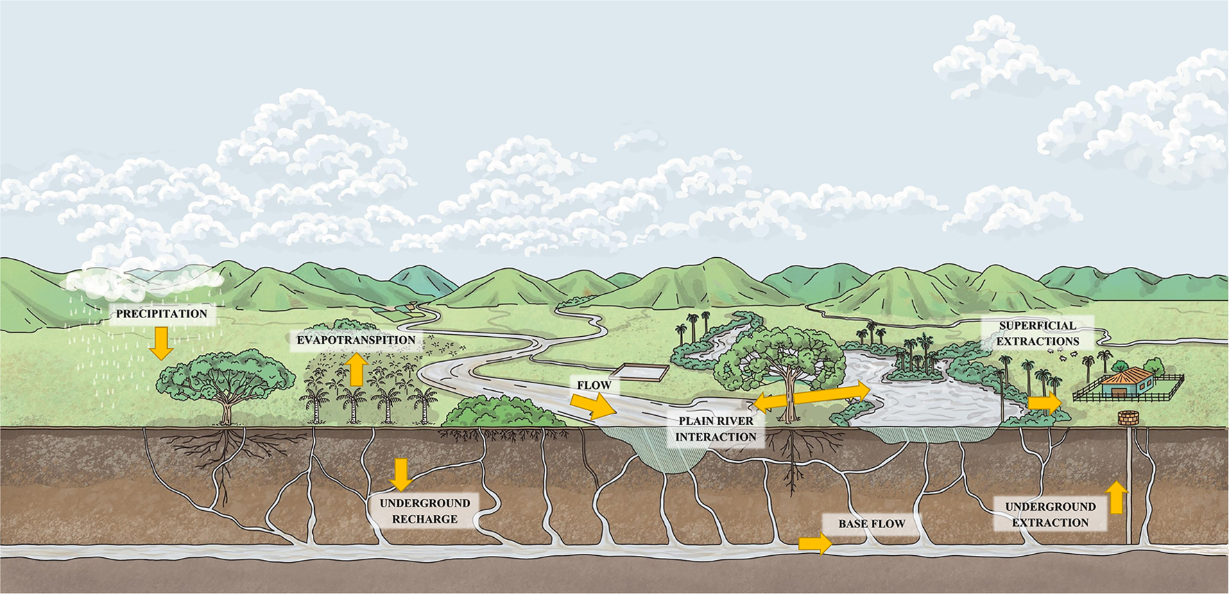
Conceptual diagram of the hydrological model.
Mathematical Model and Computational Algorithm
In accordance with the conceptual model, we reviewed 14 well known hydrological models to determine the most appropriate mathematical model in line with the scope of the research (See supplementary material). As a result of this review, we considered the ABDC hydrological model coupled with the floodplain model proposed by Angarita et al. (2018) as the best option that allows us to represent most of the conceptualized processes through a simple and parsimonious scheme. The representation of the river - floodplain interaction phenomenon is highly complex. Studies such as the one carried out by Pontes et al. (2017) show a representation of the complexity of this process based on an inertial model. In the case of the present study, the simplified conceptual model presented by Angarita et al. (2018) was chosen in order to have a simple approach to the problem.
The coupled model was configured under a semi-distributed spatial calculation scheme, considering the Hydrological Analysis Unit (HAU) as the minimum unit of analysis. To couple the ABCD model with the Angarita et al. (2018) river-floodplain interaction model, a cumulative calculation scheme was used. This implies that, at each step of time i, the water balance is solved in the j Hydrological Analysis Unit using the equations of the Thomas (1981) model.
The ABCD model (Liu, 2020; X.; Wang et al., 2020; X.; Zhang et al., 2020) considers two water storage components for the analysis of the water balance in the ; the first component represents the soil or evapotranspiration zone above the water table and the second component represents the saturated zone ( below the water table.
For modeling purposes, the subsurface flow component in the surface part of the evapotranspiration zone can be included in the direct runoff (). The model considers negligible the lateral deep flow in the unsaturated zone, in such way that the potential recharge is equaled to the real recharge .
Applying the continuity equation to a control volume :Where: , precipitation; , actual evapotranspiration; , recharge; , direct runoff; , change in soil storage between the calculation period i and the immediately preceding period (). Thomas (1981) further defines the variables (available water) and as:
In each time interval, we assume that the humidity decreases according to the exponential decay law, assuming as initial humidity at the beginning of each interval , where is the potential evapotranspiration and is a parameter of the model:
Thomas (1981) defines the state variable as a non-linear function of water available according to the parameters (dimensionless) and :Where and are parameters that can be determined from measurements of precipitation, evapotranspiration, and soil moisture in the basin. The upper limit of is represented by the parameter . Thomas (1981) notes that the function has no particular meaning. Then, when replacing in the previous equations, we obtain:
To differentiate the runoff from the recharge, a partition coefficient is assumed:
The underground flow , which is the fraction of the flow observed in the river that comes from the storage in the saturated zone , is:
The storage is interpreted as a dynamic storage that represents the connectivity between the river and the aquifer. Therefore, when applying the continuity equation to a volume of aquifer storage :Where is the change in storage of the saturated zone and is the storage of groundwater in the immediately preceding period. By substituting the previous equations and solving for :
The total flow, that is the flow observed in the river, is:
According to Thomas (1981), the parameters a, b, c, and d can be interpreted in the following way:
a is the tendency of runoff that occurs before the soil is completely saturated. Values of " a less than one generate runoff when .
b is the upper limit to the sum of the real evapotranspiration and soil moisture.
c is the fraction of the average flow of the river that comes from the groundwater.
d is the reciprocal of the residence time of the groundwater.
Having solved all the previous equations for the time step i, the flows, surface water demands, and water returns of each are accumulated. As the model accumulates, it subtracts the surface water demands from the river flow and adds the water returns. Therefore, the total flow of the river () would be given by:Where is the surface water demand and the surface water return.
Then, the model checks if there are zones with river-floodplains interaction. If there is, the model solves the equations of the Angarita et al., 2018 model as follows:Where corresponds to the accumulated flow upstream, represents the lateral flow between the river and the floodplain, represents the lateral flows between the river and the floodplain, in the area of the , is the floodplain area of , is the volume of water that the floodplain can store, and indicate the percentage of contribution in each of the directions of the interaction, and indicates the percentage of contribution in each of the directions of the river-floodplains and floodplains-river interaction.
The model leaves groundwater demand unresolved at the HAU level, requiring the use of Hydrogeological Units of Analysis (UHG). A UHG was defined as the grouping of HAUs belonging to the same hydrogeological unit. The reason groundwater demands were managed this way is because most of the time there is no correspondence between the limits of the surface basins and the limits of the aquifers.
For the water balance in groundwater storage, incorporating groundwater demands, the volume of water stored in the UHG () is calculated as the sum of the groundwater storages of the n HAU that are part of the same UHG.Where k denotes that a HAU is part of the same UHG and is the percentage of water demand that is supplied by groundwater.
Model Configuration for the Colombian Orinoquia
The modeling framework used the Arc Hydro Tools package in ArcGIS10.3, generating 4,273 HAUs with an accumulation threshold of 10 km2. Computationally, the model interprets a HAU as a modeling node and represents the basin segment as a graph. Thus, the framework assigned unique codes to each HAU, establishing connectivity between neighboring HAUs. We assigned the climatic and water demand variables to each unit individually.
In the period from 1985 to 2014, the precipitation and temperature fields were generated at monthly temporal resolution, with a pixel size of 250 m. We used Ordinary Kriging methodology for precipitation and multiple linear regressions for temperature to supply this data. In total, 360 raster files were generated. As a synthesis, Figure 3 shows the averages of each variable.
FIGURE 3
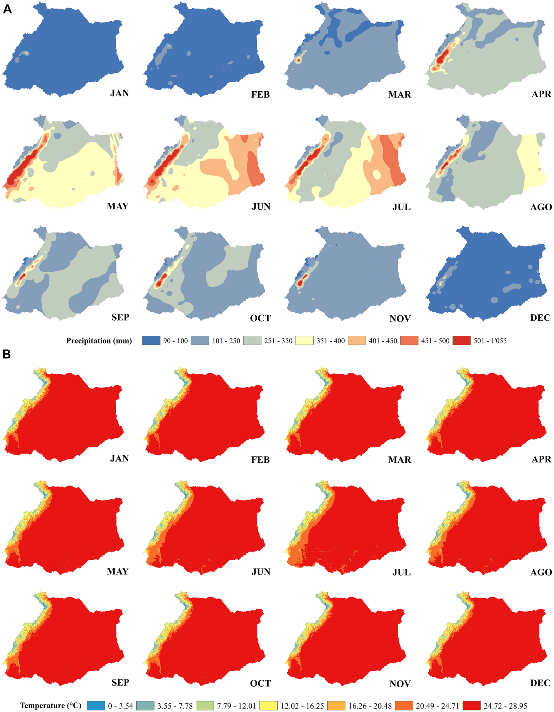
(A) multi-year monthly total precipitation fields and (B) multi-year monthly mean temperature fields.
The potential evapotranspiration was estimated using the Thornthwaite and Mather (1957) methodology. The water demands were integrated individually for each sector.
For the evaluation of the scenarios, we assumed that the climatic conditions remain constant in time and space, evaluated with the climatic series of the baseline condition (historical record).
Calibration and Validation
We used the Shuffled Complex Evolution (SCE-UA) heuristics proposed by Duan et al. (1994) to calibrate the hydrological model. Thus, a total of 57 flow measurements were used whose series were verified to be homogeneous and consistent (Figure 4).
FIGURE 4
Groups of HAUs related to flow stations. Uncalibrated HAUs are shown as gray polygons.
In total, 9 parameters (a, b, c, d, Ext, Qthreshold, Vthreshold, Trf, Tfr) were calibrated in each HAU with the presence on floodplains and 5 parameters (a, b, c, d, Ext) in the HAU remaining. For the segmentation of the calibration and validation periods, the traditional approach of 70% of the data to calibrate and 30% to validate was used. However, in the stations that did not have sufficiently extensive series, no validation was performed, so the entire data was used for calibration. The time periods used for each phase can be consulted in the supplementary material. The performance metric that was used in the calibration process was the Nash-Sutcliffe coefficient (NSE). However, metrics such as Absolute Mean Error (AME), Differential of Peak Events (PDIFF), Mean Absolute Error (MAE), Mean Square Error (MSE), Root Mean Square Error (RMSE), Fourth Root of the Mean Error Raised to the Fourth Power (R4MS4E), Root of Absolute Error (RAE) and Percentage Error in Peaks (PEP) were estimated (Teegavarapu and Elshorbagy, 2005; Dawson et al., 2007). Table 1 shows the performance metrics evaluated.
TABLE 1
| Symbology | Mathematic expression | Name |
|---|---|---|
| NSE (Ad) | Nash-Sutcliffe coefficient | |
| AME (m3/s) | Absolute Mean Error | |
| PDIFF (m3/s) | Differential of peak events | |
| MAE (m3/s) | Mean Absolute Error | |
| MSE (m3/s)2 | Mean Square Error | |
| RMSE (m3/s) | Root Mean Square Error | |
| R4MS4E (m3/s) | Fourth Root of the Mean Error Raised to the Fourth Power | |
| RAE (Ad) | Root of Absolute Error | |
| PEP (%) | Percentage Error in Peaks |
Performance metrics evaluated.
In the following equations, is the observed value, is the modelled value (where i = 1 to n data points) and is the mean of the observed data
Given the nature of the hydrological model, the calibration was carried out under a cumulative scheme, homogeneously calibrating the HAUs up to the closure point with a flow gauge. Figure 5 presents a conceptual example of the process used. It shows the HAUs associated with three flow gauges.
FIGURE 5
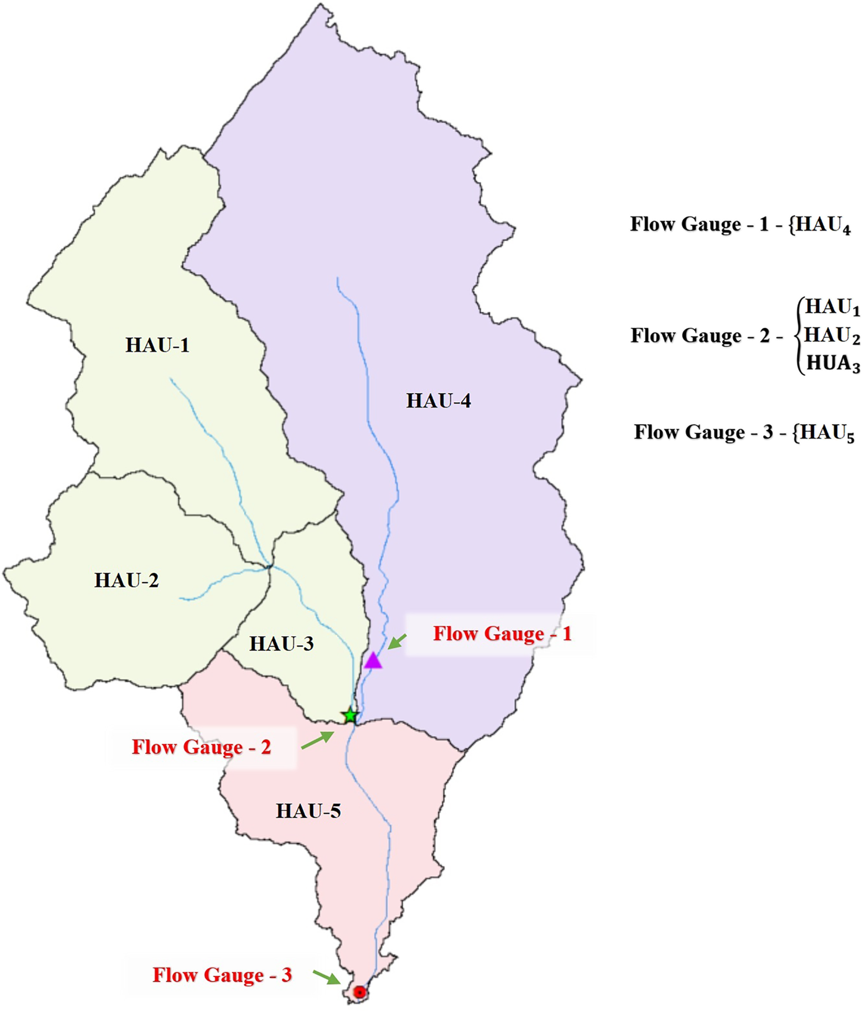
Cumulative calibration scheme.
Knowing that flow gauges one and two are of order 1 (they do not have upstream stations) and flow gauge three is of order 2 (it has one upstream station in line on the same main channel), the calibration process starts hierarchically from the HAUs associated with gauges of order 1, to those of order n. Note that in the example presented in Figure 5, HAU-1, HAU-2 and HAU-3 share the same set of parameters, since they have flow gauge 2 as the gauge in the closure point that can bring flow measurement data for the calibration of these three HAUs. For the proposed model, there were 12 hierarchy orders associated with the available flow gauges. In the HAUs where there were no flow stations, the parameters were regionalized by similarity of morphometric characteristics with calibrated HAUs. Figure 4 shows the HAU groups related to the flow stations used in the calibration. Uncalibrated HAUs are marked in gray.
As part of the analysis, we proposed an evaluation of the model exploring its performance, the suitability of its structure, the identifiability of its parameters, and the uncertainty of its predictions. To this end, 10,000 Monte-Carlos simulations were carried out using the Latin hypercube sample (LHS) method and the responses of the model were analyzed with the Monte Carlo Analysis Toolbox (MCAT) (Wagener et al., 2002) using dotty plots, regional sensitivity analysis and Generalized Likelihood Uncertainty Estimation (GLUE) (Beven and Binley, 1992).
Scenario Simulation
Four land use transformation scenarios were generated for the Colombian Orinoquia region, using Williams et al. (2020) framework (Figure 6). Scenarios one to four are based on historical commodity trends, existing policies, and stakeholder views, ranging from least to greatest intervention. Scenario 1 may be considered as business as usual, representing a modest expansion that is optimally generated in terms of maximizing agricultural benefits. Scenario two represents the vision of small farmers, ranchers, and agricultural industry on Colombia Orinoquia region. Scenario three represents the vision of the Colombian government described in the Master Plan (DNP, 2016), which seeks to maximize the underutilized land for agriculture. Finally, scenario four represents an extreme vision in which the entire agricultural Frontier is occupied even if it is a protected area. Below, a brief description of each of the scenarios in terms of percentage change in the Orinoco basin area of Colombia:
FIGURE 6
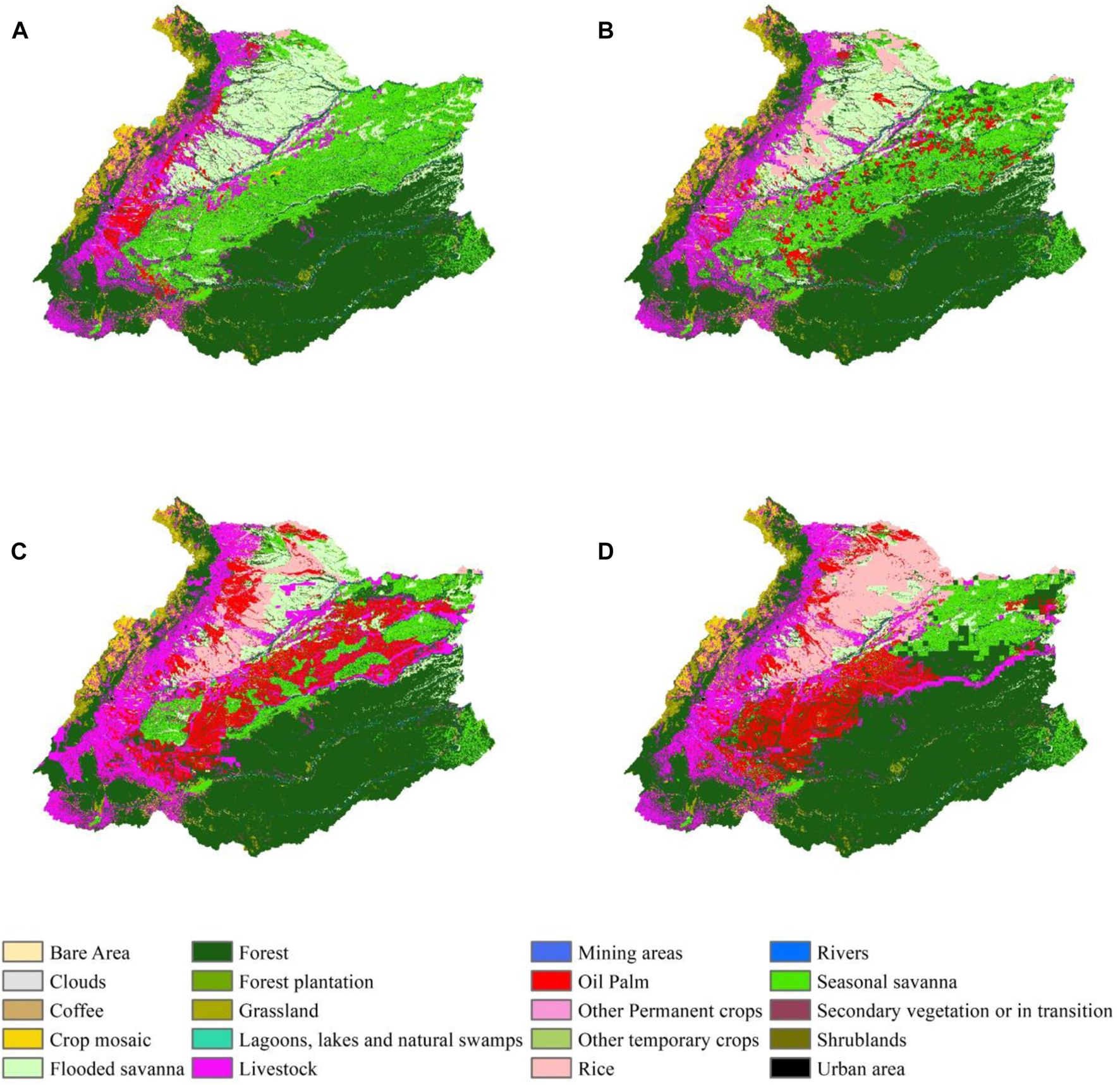
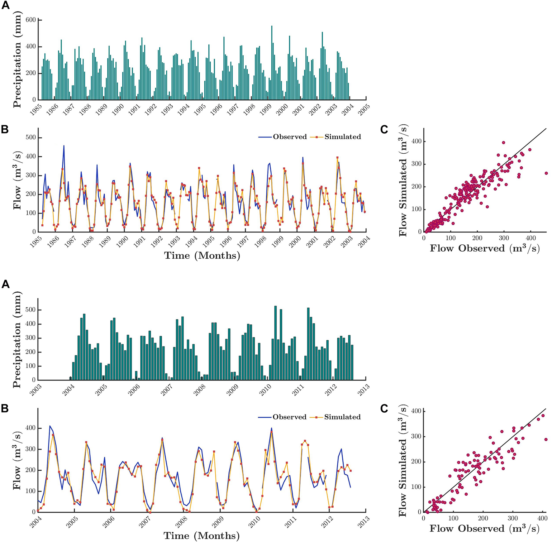
Land use transformation scenarios (A) Scenario 1, (B) Scenario 2, (C) Scenario three and C) Scenario 4. Derived from Williams et al., 2020. Calibration (A) shows the average rainfall of the HAU until closure with station 35107030 (B) shows the comparison of time series of observed flow (blue) and simulated flow (orange) and (C) shows the comparative scatter plot in the observed flow and simulated flow. Validation (A) shows the average rainfall of the HAU until closure with station 35107030 (B) shows the comparison of time series of observed flow (blue) and simulated flow (orange) and (C) shows the comparative scatter plot in the observed flow and simulated flow.
Scenario-1: This “business as usual” scenario defined expansion of 1.51% of oil palm, 0.12% of rice, 0.08% of forestry and 0.04% of soybeans.
Scenario-2: This scenario established 14.27% of the landscape to become agriculture dividing the area equally between the five basic products (oil palm, rice, forestry, soybeans and pastures for livestock).
Scenario-3: This scenario proposes expansion of 10.61% of agriculture (which were divided equally between rice and soybeans), 13.53% of livestock, 6.97% of forestry and 12.54% of agroforestry crops (assigned to oil palm).
Scenario-4: This scenario proposes 53.68% of expansion of all productive activity (oil palm, rice, forestry, soybeans and pastures for livestock).
These scenarios were simulated using the hydrological model developed for this study.
Indicators
One of the limiting factors of agricultural development is water (Abunnour et al., 2016; Salman et al., 2020). Long periods of drought, intensified by the phenomenon of El Niño-Southern Oscillation (ENSO), characterize the Orinoco basin in Colombia (Ramos-Montaño and García-Conde, 2016; Trujillo, 2018). During times of drought, the pressures on the water resources intensify and become more evident.
In this research, we carried out a comparative analysis of the scenarios using 95% percentile of flow duration curve (Q95) as an indicator, which is associated with the flows present in times of low water. The flow duration curve (FDC) synthesizes information on the distribution and characteristics of the flow at a site, providing information for optimally managing the river’s water resources. In hydrology, a FDC is a function that describes the variability of flow at a specific site during a period of interest. Q95 represents the flows equaled or exceeded 95 percent of the time, accounting for the base flows, rather than those due to extreme rainfall events (Ridolfi et al., 2020). One of the many applications of the FDC is to quantify the capacity to satisfy catchment requests (Dingman, 1981). The idea is to compare the percentage changes in Q95 between the baseline condition (historical condition) and the four proposed scenarios:where is the normalized percentage variation of the flows of the flow duration curve, associated with the 95% percentile between the baseline scenario and k scenario, is the discharge of the flow duration curve associated with the 95% percentile of the baseline scenario and is the discharge of the flow duration curve associated with the 95% percentile of the k scenario.
Results and Discussion
Performance of the Hydrological Model
The model exhibited satisfactory results in the calibration process (Table 2). In more than 85% of the stations selected as calibration points, the model presented NSE values higher than 0.6 (Table 2), which is acceptable according to the criteria established by Moriasi et al. (2007).
TABLE 2
| Flow gauges | NSE | AME | PDIFF | MAE | MSE | RMSE | R4MS4E | RAE | PEP |
|---|---|---|---|---|---|---|---|---|---|
| 31097020 | 0.85 | 2,345.93 | 1,117.33 | 502.04 | 460,780.01 | 678.81 | 1,002.70 | 0.33 | 15.86 |
| 32037010 | 0.84 | 507.46 | 96.53 | 110.39 | 22,006.23 | 148.34 | 211.80 | 0.36 | 6.66 |
| 32067020 | 0.48 | 123.04 | 86.40 | 24.71 | 1,100.09 | 33.17 | 49.18 | 0.67 | 39.98 |
| 33077010 | 0.89 | 718.14 | -219.71 | 138.95 | 38,272.04 | 195.63 | 288.34 | 0.27 | −10.28 |
| 35017040 | 0.86 | 198.21 | 63.10 | 25.30 | 1,221.16 | 34.95 | 58.42 | 0.33 | 13.76 |
| 35027130 | 0.78 | 11.14 | 4.04 | 2.04 | 7.31 | 2.70 | 3.99 | 0.44 | 14.86 |
| 35057010 | 0.80 | 95.05 | 46.20 | 23.91 | 965.36 | 31.07 | 42.37 | 0.41 | 16.82 |
| 35067010 | 0.72 | 8.95 | 5.78 | 1.58 | 4.91 | 2.22 | 3.48 | 0.47 | 28.31 |
| 35067030 | 0.73 | 4.62 | -0.35 | 1.15 | 1.98 | 1.41 | 1.84 | 0.50 | −3.23 |
| 35067050 | 0.64 | 35.78 | 35.78 | 8.06 | 122.46 | 11.07 | 16.21 | 0.54 | 40.26 |
| 35087020 | 0.80 | 69.01 | 39.87 | 12.19 | 287.52 | 16.96 | 26.01 | 0.41 | 23.37 |
| 35087030 | 0.84 | 8.99 | 6.31 | 1.44 | 4.19 | 2.05 | 3.23 | 0.35 | 24.37 |
| 35097090 | 0.72 | 138.85 | 94.72 | 18.64 | 837.93 | 28.95 | 49.52 | 0.43 | 36.36 |
| 35107010 | 0.70 | 68.88 | 51.58 | 16.08 | 451.58 | 21.25 | 28.89 | 0.49 | 30.18 |
| 35127020 | 0.85 | 74.99 | 49.72 | 20.77 | 642.08 | 25.34 | 32.85 | 0.37 | 19.53 |
| 35137010 | 0.76 | 100.64 | 54.68 | 18.06 | 623.60 | 24.97 | 37.72 | 0.41 | 25.97 |
| 35197020 | 0.66 | 16.30 | 12.96 | 2.42 | 12.45 | 3.53 | 5.65 | 0.50 | 43.33 |
| 35217010 | 0.69 | 125.84 | 60.49 | 20.50 | 854.54 | 29.23 | 45.31 | 0.48 | 25.86 |
| 35217060 | 0.82 | 84.28 | 59.07 | 18.58 | 699.05 | 26.44 | 38.77 | 0.35 | 23.51 |
| 35227090 | 0.71 | 54.31 | 22.80 | 10.50 | 224.51 | 14.98 | 21.47 | 0.46 | 21.70 |
| 36027050 | 0.72 | 485.62 | 282.83 | 144.72 | 32,410.09 | 180.03 | 236.57 | 0.48 | 22.22 |
| 32037030 | 0.87 | 705.79 | 460.17 | 145.85 | 39,235.34 | 198.08 | 290.12 | 0.31 | 19.52 |
| 32077080 | 0.82 | 360.25 | 289.95 | 69.91 | 9,007.66 | 94.91 | 137.31 | 0.39 | 25.39 |
| 32077100 | 0.83 | 92.63 | 31.35 | 17.03 | 508.53 | 22.55 | 32.47 | 0.37 | 12.32 |
| 35017050 | 0.63 | 199.64 | 141.61 | 64.47 | 6,342.76 | 79.64 | 101.89 | 0.62 | 25.77 |
| 35027200 | 0.76 | 53.14 | 45.56 | 12.58 | 258.95 | 16.09 | 21.85 | 0.47 | 28.10 |
| 35127030 | 0.85 | 303.84 | 116.07 | 77.31 | 10,982.85 | 104.80 | 142.56 | 0.33 | 11.24 |
| 35197190 | 0.76 | 43.35 | 38.63 | 8.12 | 152.98 | 12.37 | 19.14 | 0.40 | 35.67 |
| 35217020 | 0.85 | 259.94 | 149.10 | 48.51 | 4,226.84 | 65.01 | 96.26 | 0.33 | 21.58 |
| 37057020 | 0.79 | 432.74 | 263.83 | 98.33 | 17,069.41 | 130.65 | 183.27 | 0.42 | 20.19 |
| 32047010 | 0.88 | 1,148.61 | 459.86 | 211.11 | 81,434.37 | 285.37 | 413.89 | 0.30 | 13.49 |
| 32077070 | 0.91 | 101.20 | 11.93 | 22.65 | 896.42 | 29.94 | 41.13 | 0.28 | 2.87 |
| 35027140 | 0.87 | 91.25 | 53.32 | 23.73 | 956.03 | 30.92 | 41.94 | 0.33 | 13.89 |
| 35107020 | 0.86 | 341.73 | 165.44 | 70.86 | 9,991.91 | 99.96 | 151.01 | 0.31 | 13.95 |
| 35127010 | 0.89 | 344.87 | 284.50 | 86.24 | 13,307.61 | 115.36 | 159.23 | 0.29 | 20.51 |
| 35197180 | 0.62 | 505.95 | 505.95 | 86.48 | 16,395.05 | 128.04 | 197.87 | 0.50 | 52.59 |
| 32087040 | 0.86 | 521.48 | 333.39 | 99.46 | 17,679.63 | 132.96 | 194.40 | 0.34 | 18.87 |
| 35017020 | 0.89 | 296.38 | 166.46 | 60.40 | 6,319.64 | 79.50 | 113.17 | 0.30 | 16.02 |
| 32107010 | 0.90 | 1,239.57 | 383.38 | 295.90 | 157,307.26 | 396.62 | 547.48 | 0.28 | 7.46 |
| 35107030 | 0.91 | 489.12 | 236.26 | 115.76 | 22,543.74 | 150.15 | 205.12 | 0.27 | 11.25 |
| 32117010 | 0.81 | 2,296.69 | 930.91 | 468.19 | 385,306.70 | 620.73 | 887.36 | 0.39 | 14.81 |
| 35117010 | 0.94 | 855.62 | 790.08 | 159.39 | 46,195.98 | 214.93 | 307.34 | 0.21 | 20.18 |
| 35177020 | 0.92 | 1,234.27 | 502.21 | 275.40 | 135,547.28 | 368.17 | 508.07 | 0.24 | 9.73 |
| 32157040 | 0.87 | 1883.26 | 242.15 | 530.26 | 499,000.19 | 706.40 | 947.10 | 0.32 | 3.52 |
| 35267030 | 0.91 | 1927.53 | 228.97 | 450.81 | 328,928.77 | 573.52 | 762.31 | 0.27 | 3.09 |
| 32157060 | 0.85 | 2,626.58 | 722.37 | 563.98 | 560,156.52 | 748.44 | 1,030.58 | 0.33 | 9.62 |
| 35267080 | 0.89 | 2,751.98 | 1,356.46 | 590.67 | 628,550.28 | 792.81 | 1,120.45 | 0.28 | 13.92 |
| 32207010 | 0.79 | 3,873.76 | 843.62 | 766.42 | 1037913.69 | 1,018.78 | 1,485.56 | 0.40 | 9.08 |
| 35257040 | 0.90 | 3,835.63 | 2,673.93 | 731.58 | 988,289.03 | 994.13 | 1,463.38 | 0.26 | 19.71 |
| 31097010 | 0.89 | 4,960.51 | 738.07 | 1,018.32 | 1,755,459.12 | 1,324.94 | 1879.42 | 0.29 | 4.83 |
Model performance metrics in calibration.
As an example, Figure 7 shows the graphic results of the calibration at the control point established by El Barro station [35017040]. It shows the ability of the model to reproduce the dynamics of the hydrological regime draining to this control point. It also expresses the performance of the model in estimating the flow values in each of the seasons of the hydrological regime. This performance is reflected in the coefficient of determination (0.89) which highlights the capacity of the model in terms of the representation of the hydrological regime (1 being the highest value that this metric can reach). Metrics such as PDIFF (63.1 m3 s−1), the R4MS4E (58.4 m3 s−1) and the PEP (13.7%) demonstrate the degree of precision with which the model hits the peak values in El Barro station [35017040]. On the other hand, metrics such as MAE show that the average errors of these estimates do not exceed 25.3 m3 s−1. The quality and quantity of the information also represent an important factor in the performance of the model. Poor information leads to models that spread errors, generating greater uncertainty in the results.
FIGURE 7
Comparative graphs in the calibration (1) and validation (2) at El Barro station [35017040].(A) Dotty plot graph of the variation of the objective function in the evaluation range of the parameters (a is runoff, b is upper limit of evapotranspiration and soil moisture, c. is groundwater fraction, d is reciprocal of groundwater residence time, and indicate the percentage of contribution in each of the directions of the interaction, and indicates the percentage of contribution in each of the directions of the river-floodplains and floodplains-river interaction and is the percentage of water demand that is supplied by groundwater).(B) Graphs of parametric regional sensitivity, in red the objective functions with the lowest performance of the model, in blue the objective functions with the highest performance of the model.(C) Uncertainty using the Generalized Likelihood Uncertainty Estimation method (Beven & Binley, 1992).
The scatter plot presented in Figure 8A shows that the model has a low identifiability of its parameters, except parameters a and b that show a slight concavity indicating that they can be identified. The regional sensitivity graphs (Figure 8B) present the cumulative distributions of the evaluated parameters ranked from best to worst in terms of the objective function. With the GLUE methodology (Beven and Binley, 1992), the evaluated parameters are divided into ten groups of equal size according to the value of the objective function. The cumulative distribution of each group is represented as the probability value compared to the parameter values. The higher the gradient, the higher the sensitivity of the parameter. For this particular case, the only parameters that are sensitive are a and b.
FIGURE 8
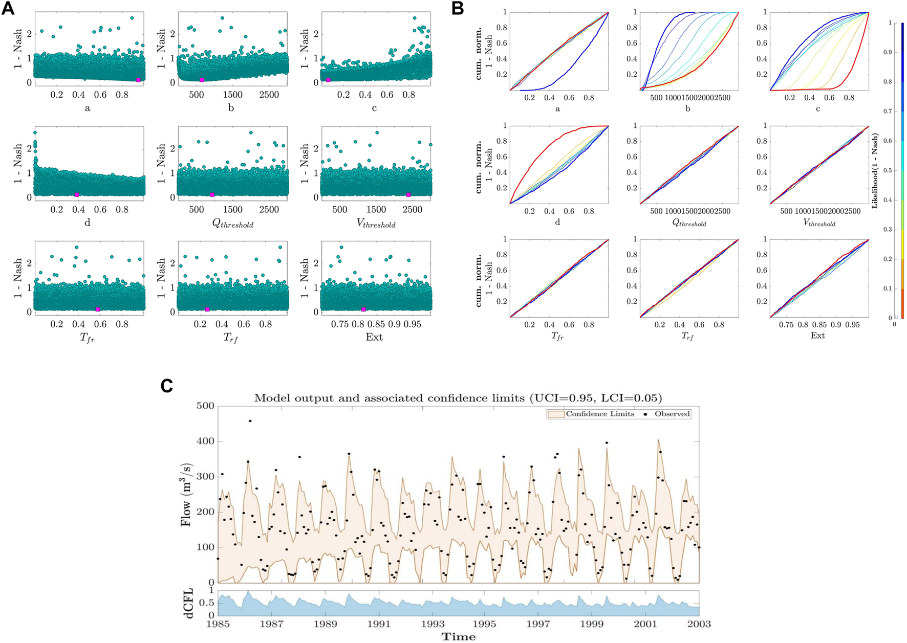
(A) Dotty plots objective function (1-), (B) Regional sensitivity plot (1-) and (C) Generalized Likelihood Uncertainty Estimation (GLUE) for El Barro station [35017040].
Figure 8C shows that the 90% confidence band contains most of the observed data, indicating that the structure of the model is capable of correctly representing the measured data. However, there are observations in periods of high flow, which are outside the confidence limits. This situation may be due to the uncertainty that exists in the measurement of flow rates, since the estimation is already made by means of a rating curve (Sikorska and Renard, 2017), a characteristic widely evidenced in hydrological modeling exercises (Ibarra et al., 2016; Shen et al., 2012; Yang et al., 2018). Another factor that can explain this behavior is the incomplete representation of the spatial variability of precipitation, as a consequence of limited monitoring in most of the Orinoco basin in Colombia. Figure 8C shows that the confidence band is wide, which denotes the parametric uncertainty that the model presents.
Scenarios
Figure 9 shows the spatial distribution of the normalized percentage variations of Q95 for the four land use transformation scenarios.
FIGURE 9
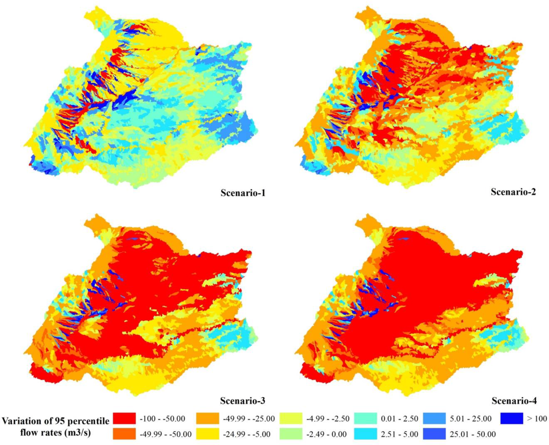
Spatial distribution of the normalized percentage variations of the flows associated with the 95th percentile (Q95) of the flow duration curve for the analysis scenarios.
These results show that the changes in coverage and land use derived from the four scenarios generate an important impact on the water availability of the Orinoquia (with reductions greater than 50% in discharge during dry periods). In order of impact, scenario one turns out to be the mildest, while scenario four is the most drastic.
In scenario 1, most of the agro-industrial expansion is concentrated in a narrow northeast to southwest band of the flooded savannas of the departments of Casanare and Arauca, causing reductions of more than 50% in discharge during dry periods (shown in red in Figure 9, Scenario-1). However, in departments like Vichada, where protected areas and natural ecosystems predominate, the results showed increases in Q95 ranging from 5 to 25% in most HAUs. At the regional level, this scenario causes a 28% reduction in Q95 in the Meta River at the mouth with the Orinoco river.
The results of scenario two showed that the impacts on the water resource are greater than in scenario 1, extending throughout the department of Arauca, Casanare, part of Vichada and Meta. In this scenario, the Meta River at its mouth with the Orinoco River shows a reduction of 83% in Q95, in addition, tributaries such as the Guaviare River (at the confluence with the Inírida River) and the Vichada River (at the confluence with the Orinoco River) present reductions of 10 and 15% in Q95 respectively.
Scenarios three and four are the most unfavorable in terms of water resources given their expansion objective of 151,528 km2 and 186,380 km2 respectively. These two scenarios show a reduction of more than 50% in Q95, in 50% of the entire Orinoco basin in Colombia. In scenario 3, the Meta and Vichada rivers at their mouths with the Orinoco river and the Guaviare river at the confluence with the Inírida river, show reductions in flow of 95, 98 and 50% in Q95 respectively, while the same rivers for scenario four show reductions of 97, 95 and 48% in Q95 respectively.
An important characteristic that is general to all the evaluated scenarios is the extensive development evidenced over the flooded savannas, mainly by livestock and rice and oil palm crops. These developments affect the connectivity and water regulation capacity of the watersheds. They result from extensive logging, removal of vegetation cover, soil plowing and burning processes, all of which reduce the forests of the foothills and plains (Svenson, 1996; Tamaris et al., 2017), Although scenarios three and four present the greatest effects, the soil’s physical and chemical limitations make these scenarios very costly economically, but not necessarily less likely (BuriticáMora et al., 2015; Osorio-Peláez, 2015;, 2016; Bustamante, 2019).
The results obtained in the scenario analysis indicate changes in the hydrological regimes of the Colombian Orinoco basin that can generate direct impacts on biodiversity and ecosystems. The unique ecosystem of the flooded savannas support about 250 species of mammals, 567 species of fish, 761 species of birds, more than 700 species of plants, 108 species of amphibians and 119 species of reptiles in the Colombian Orinoco basin (Mora et al., 2015; Buriticá, 2016). A potential agroindustrial expansion in the Orinoquia region can reduce flooded savannas inundation and could have a great impact on the density and size of the populations and organisms that depend on flooded savannas (Kingsford and Thomas, 1995). For example, during 2014, in the department of Casanare, a region where more than 50% of its area is flooded savannas, there was a decrease in the quality of the habitat for Hydrochoerus hydrochaeris (capybara in English and Chigüiro in Spanish, the world’s largest rodent) due to the scarcity of water, which generated a physiological pressure on the population and the subsequent death of a large number of individuals (Semana, 2014). The availability of water is one of the most important factors in the quality of habitat of the Hydrochoerus hydrochaeris (López-Arévalo et al., 2014). An agroindustrial expansion without considering the ecological limits of sustainability for ecosystems and species may generate great impacts that could put this delicate ecosystem at risk.
New water demands can generate reductions in the magnitude of the base flows, leading to biodiversity and ecosystem change. These water availability changes might include a decrease in the size of a population or local extinction of species (Kupferberg et al., 2012), reduction of species richness (Benejam et al., 2010) or terrestrial species invasion in the riparian and canal zone (Stromberg et al., 2007). Due to limits on water availability, agriculture and biodiversity conservation may be in conflict, especially during dry periods in areas with large monocultures. Poor water quality is another factor limiting usefulness of water. In rural areas of the Orinoquia, the population collects water directly from the rivers near their homes. Excessive use of agrochemicals in rice and palm crops may limit domestic water use (Reyes, 2020). This same situation affects ranchers who practice extensive cattle ranching.
The hydrological model demonstrated in this study allows decision makers to assess in advance potential conflicts related to the quantity and availability of water. It provides information on the amount of water in the 4,273 HAU, data that is essential for water allocation and planning. The model also allows us to understand how flows are reduced month by month when the water requirements of the hydro dependent water use sectors are increased, not only in the units where water is extracted, but also downstream of these units. If the model is combined with environmental or ecological analysis, planners can more efficiently allocate water across the basin and throughout the year, minimizing negative effects on ecosystems.
Conclusion
The coupling of the Thomas (1981) model and the Angarita et al. (2018) floodplain river interaction model demonstrated satisfactory results according to the performance metrics obtained in the calibration (NSE from 0.62 to 0.92) and validation (NSE from 0.49 to 0.92) exercises. Although the results of the sensitivity analysis showed that the parameters of the river-floodplain interaction model are not sensitive, the model allows, in a simplified way, to represent the natural dynamics that occur in the Colombian Orinoquia. In addition, the results of the Generalized Likelihood Uncertainty Estimation (GLUE) demonstrated that the model can structurally represent the flows recorded in the Colombian Orinoquia.
Sensitivity and parametric uncertainty analyses are necessary for any valid assessment of hydrological processes. Tools such as MCAT facilitate these processes, improving our understanding of how the model reacts to input signals and if its equations are adequate to represent hydrological records in the field.
The adopted calibration scheme allowed the model to be parameterized in such a way that the representation of the hydrological dynamics of the Colombian Orinoquia was consistent with the records in the hydrological stations used in the calibration exercise. However, despite the parameters being clearly effective for calibration, they do not fully capture the characteristics of the basin. This is directly linked to parametric equifinality problems. For future work, a calibration scheme could be explored that relaxes the requirements of the basin hierarchy scheme use in this study, in favor of orienting the model towards biophysical processes.
Future efforts building on our hydrological model could be focused on capturing physical properties and their interactions with management practices. Moreover, among the opportunities to improve the hydrological model is the need to implicitly couple the demands of surface water with the equations that describe soil moisture decay, as well as groundwater demands with equations describing groundwater loss. The incorporation of processes such as rain interception could also improve the representation of the hydrological cycle. However, the objective of maintaining parametric parsimony and simplicity in the configuration of the model should not be overlooked.
The Colombian Orinoquia is considered the last agricultural Frontier of the country. Unplanned and intensive development, where the objectives of agricultural production and those of the ecosystems are unbalanced, can have serious repercussions on the water resource (decreases of more than 50% in discharge during dry periods). Lack of planning could compromise water security and put the ecological integrity of the Orinoquia at risk, as evidenced by model results of scenarios three and 4. Therefore, it is essential to integrate hydrological analysis in planning processes. In addition, planning must consider multiple scales, with analysis at the macro-region level (such as those addressed in this study) and at more detailed scales.
Statements
Data availability statement
The original contributions presented in the study are included in the article/Supplementary Materials, further inquiries can be directed to the corresponding author.
Author contributions
Conceptualization, JN, CR, TW; Investigation, JN, CR; Methodology, JN, CR; Writing-original draft, JN; Writing-review and editing, JN, CR, TW. All authors have read and agreed to the published version of the manuscript.
Acknowledgments
This study was part of a collaborative SNAPP (Science for Nature and People Partnership) project titled “Land use change in the Orinoquia” between the University of Queensland (UQ), Wildlife Conservation Society (WCS), The Nature Conservancy (TNC) and International Center for Tropical Agriculture (CIAT). We thank Andrés A. Roa for suggestions that improved the manuscript. We also thank the independent reviewers and editors for comments and suggestions.
Conflict of interest
The authors declare that the research was conducted in the absence of any commercial or financial relationships that could be construed as a potential conflict of interest.
Publisher’s note
All claims expressed in this article are solely those of the authors and do not necessarily represent those of their affiliated organizations, or those of the publisher, the editors and the reviewers. Any product that may be evaluated in this article, or claim that may be made by its manufacturer, is not guaranteed or endorsed by the publisher.
Supplementary material
The Supplementary Material for this article can be found online at: https://www.frontiersin.org/articles/10.3389/fenvs.2021.673215/full#supplementary-material
References
1
AbunnourM. A.HashimN. B. M.Bin JaafarM. (2016). Agricultural Water Demand, Water Quality and Crop Suitability in Souk-Alkhamis Al-Khums, Libya. IOP Conf. Ser. Earth Environ. Sci.37, 012045. 10.1088/1755-1315/37/1/012045
2
ACP. (2017). Informe Estadistico Petrolero. Available at: https://www.resourcedata.org/dataset/rgi-informe-estadistico-petrolero.
3
AndradeG. I.CastroL. G. (2012). Degradación, pérdida y transformación de la biodiversidad continental en Colombia, invitación a una interpretación socioecológica. En Ambiente y Desarrollo XVI (30)53, 71.
4
AngaritaH.WickelA. J.SieberJ.ChavarroJ.Maldonado-OcampoJ. A.Herrera-R.G. A.et al (2018). Basin-scale Impacts of Hydropower Development on the Mompós Depression Wetlands, Colombia. Hydrol. Earth Syst. Sci.22 (5), 2839–2865. 10.5194/hess-22-2839-2018
5
ANM (2018). Informe de producción de minerales del 2015. Available at: https://www1.upme.gov.co/simco/Cifras-Sectoriales/paginas/informacion-estadistica-minera.aspx.
6
BedoyaM.ContrerasC.RuizF. (2010). Estudio Nacional del Agua (ENA). In Estudio nacional del agua. Colombia: Publicación aprobada por el Comité de Comnicaciones y Publicaciones del IDEAM.
7
BenejamL.AngermeierP. L.MunnéA.García-berthouE. (2010). Assessing Effects of Water Abstraction on Fish Assemblages in Mediterranean Streams. Freshw. Biol.55 (3), 628–642. 10.1111/j.1365-2427.2009.02299.x
8
BevenK.BinleyA. (1992). The Future of Distributed Models: Model Calibration and Uncertainty Prediction. Hydrol. Process.6 (3), 279–298. 10.1002/hyp.3360060305
9
BuriticáN. (2016). Sabanas Inundables de la Orinoquía Colombiana. GIZ Colombia: Instituto de Investigación de Recursos Biológicos Alexander von Humboldt.
10
BustamanteC. (2019). Gran Libro de la Orinoquia Colombiana. GIZ Colombia: Instituto de Investigación de Recursos Biológicos Alexander von Humboldt.
11
ByardJ. L. (1999). The Impact of Rice Pesticides on the Aquatic Ecosystems of the Sacramento River and Delta (California). Impact Rice Pestic. Aquat. Ecosyst. Sacramento River Delta (California), 95–110. 10.1007/978-1-4612-1496-0_4
12
Cárdenas-SantamaríaM.Hernández-CorreaG.Maiguashca-OlanoA. F.Meisel-RocaA.Ocampo-GaviriaJ. A.Zárate-PerdomoJ. P.et al (2018). Report of the Board of Directors to the Congress of the Republic - March de 2018. Bogotá, DC: Banco de la República de Colombia. Available at: https://repositorio.banrep.gov.co/handle/20.500.12134/9559.
13
CravenJ.AngaritaH.Corzo PerezG. A.VasquezD. (2017). Development and Testing of a River basin Management Simulation Game for Integrated Management of the Magdalena-Cauca River basin. Environ. Model. Softw.90, 78–88. 10.1016/j.envsoft.2017.01.002
14
DANE (2008). Censo General 2005. Available at: https://www.dane.gov.co/index.php/estadisticas-por-tema/demografia-y-poblacion/censo-general-2005-1.
15
DawsonC. W.AbrahartR. J.SeeL. M. (2007). HydroTest: A Web-Based Toolbox of Evaluation Metrics for the Standardised Assessment of Hydrological Forecasts. Environ. Model. Softw.22 (7), 1034–1052. 10.1016/j.envsoft.2006.06.008
16
DingmanS. L. (1981). PLANNING LEVEL ESTIMATES OF THE VALUE OF RESERVOIRS FOR WATER SUPPLY AND FLOW AUGMENTATION IN NEW HAMPSHIRE. J. Am. Water Resour. Assoc17 (4), 684–690. 10.1111/j.1752-1688.1981.tb01277.x
17
DNP (2018). Bases del Plan Nacional de Desarrollo 2018-2022.
18
DNP (2016). Plan Maestro de la Orinoquia. Available at: https://colaboracion.dnp.gov.co/CDT/Prensa/PND-2018-2022.pdf%0AGoogle%Scholar.
19
DuanQ.SorooshianS.GuptaV. K. (1994). Optimal Use of the SCE-UA Global Optimization Method for Calibrating Watershed Models. J. Hydrol.158 (3–4), 265–284. 10.1016/0022-1694(94)90057-4
20
FAO (2017). Water for Sustainable Food and Agriculture. Available at: http://www.fao.org/3/i7959e/i7959e.pdf.
21
GassónR. A. (2002). Orinoquia: the Archaeology of the Orinoco River Basin. J. World Prehistory16 (3), 237–311. 10.1023/a:1020978518142
22
BrierleyG. J.FryirsK. A. (Editors) (2004). Geomorphology and River Management (Malden, MA: Blackwell Publishing). 10.1002/9780470751367
23
IbarraS.RomeroR.PoulinA.GlausM.CervantesE.BravoJ.et al (2016). Sensitivity Analysis in Hydrological Modeling for the Gulf of México. Proced. Eng.154, 1152–1162. 10.1016/j.proeng.2016.07.531
24
ICA (2016). Censo Pecuario Nacional - 2016. Bogotá, DC: Instituto Colombiano Agropecuario. Available at: https://www.ica.gov.co/getdoc/8232c0e5-be97-42bd-b07b-9cdbfb07fcac/censos-2008.aspx.
25
IDEAM (2019). Estudio Nacional del Agua 2018. Bogotá: Ideam, 452.
26
JunkW. J.BayleyP. B.SparksR. E. (1989). “The Flood Pulse Concept in River-Floodplain Systems,” in Proceedings of theInternational Large River Symposium. Can. Spec. Public Fish. Aquat. Sci.. Editors DodgeD. P.106.
27
KanianskaR. (2016). Agriculture and its Impact on Land‐Use, Environment, and Ecosystem Services. Landscape Ecology - the Influences of Land Use and Anthropogenic Impacts of Landscape Creation. Banská Bystrica, Slovakia: InTech. 10.5772/63719
28
KingsfordR. T.ThomasR. F. (1995). The Macquarie Marshes in Arid Australia and Their Waterbirds: a 50-year History of Decline. Environ. Manage.19 (6), 867–878. 10.1007/bf02471938
29
KupferbergS. J.PalenW. J.LindA. J.BobzienS.CatenazziA.DrennanJ.et al (2012). Effects of Flow Regimes Altered by Dams on Survival, Population Declines, and Range-wide Losses of California River-Breeding Frogs. Conservation Biol.26 (3), 513–524. 10.1111/j.1523-1739.2012.01837.x
30
López-ArévaloH. F.Sánchez-PalominoP.MontenegroO. L. (2014). El chigüiro Hydrochoerus hydrochaeris en la Orinoquía colombiana: Ecología, manejo sostenible y conservación. Biblioteca José Jerónimo Triana. Bogotá: Instituto de Ciencias Naturales. Universidad Nacional de Colombia435.
31
Labrador CadenaA. F.Zúñiga L.J. M.Romero C.J. (2016). Desarrollo de un modelo para la planificación integral del recurso hídrico en la cuenca hidrográfica del Río Aipe, Huila, Colombia. Ingeniería y Región15, 23. 10.25054/22161325.1176
32
LiuD. (2020). A Rational Performance Criterion for Hydrological Model. J. Hydrol.590, 125488. 10.1016/j.jhydrol.2020.125488
33
MinAgricultura (2018). Evaluaciones Agropecuarias - EVA. Available at: https://www.agronet.gov.co/estadistica/paginas/home.aspx?cod=59.
34
Mora-FernándezC.Peñuela-RecioL.Castro-LimaF. (2015). Estado del conocimiento de los ecosistemas de las sabanas inundables en la Orinoquia Colombiana. Orinoquia19 (2), 253–271. 10.22579/20112629.339
35
MoriasiD. N.ArnoldJ. G.Van LiewM. W.BignerR. L.HarmelR.VeithT. L. (2007). Evaluation Guidelines for Systematic Quantification of Accuracy in Watershed Simulation. Am. Soc. Agric. Biol. Eng.50 (23351), 885–900. 10.13031/2013.23153
36
Osorio-PeláezC. (2015). XIII. Aplicación de criterios bioecológicos para la identificación, caracterización y establecimiento de límites funcionales en humedales de las sabanas inundables de la Orinoquia. Bogotá, DC Colombia: Serie Editorial Recursos Hidrobiológicos y Pesqueros Continentales de Colombia. Instituto de Investigación de Recursos Biológicos Alexander von Humboldt (IAvH)426.
37
PontesP. R. M.FanF. M.FleischmannA. S.de PaivaR. C. D.BuarqueD. C.SiqueiraV. A.et al (2017). MGB-IPH Model for Hydrological and Hydraulic Simulation of Large Floodplain River Systems Coupled with Open Source GIS. Environ. Model. Softw.94, 1–20. 10.1016/j.envsoft.2017.03.029
38
PovedaGermán.GilM.QuicenoN. (1998). El ciclo anual de la hidrología de Colombia en relación con el ENSO y la NAO.pdf. In Bulletin Institute Francaise d´Etudes Andines27, 3, pp. 721–731.
39
PovedaGermán.MesaÓ. J. (1996). Las fases extremas del fenómeno ENSO ( El Niño y La Niña ). Ingenieria Hidraulica En MexicoXI (October2016), 21–37.
40
PovedaGérman.RojasW. (1997). Evidencias de la asociación entre brotes epidemcos de malaria en Colombia y el Fenomeno El Niño- oscilación del Sur. Revista Academica Colombiana de ciencias21, 421–429.
41
PovedaG. J.VelezO.MesaC.HoyosC.SalazarL.MejíaJ. (2002). Influencia de fenómenos macroclimáticos sobre el ciclo anual de la hidrología colombiana: cuantificación lineal, no lineal y percentiles probabilísticos. Meteorol. Colomb.6, 1–10.
42
RabinS. S.AlexanderP.HenryR.AnthoniP.PughT. A. M.RounsevellM.et al (2020). Impacts of Future Agricultural Change on Ecosystem Service Indicators. Earth Syst. Dynam.11 (2), 357–376. 10.5194/esd-11-357-2020
43
Ramos-MontañoC.García-CondeM. R. (2016). Características Ecosistémicas asociadas a la actividad ganadera en Arauca (Colombia): Desafíos frente al cambio climático TT - Ecosystem characteristics associated with livestock farming in the Arauca department (Colombia): challenges regarding climate c. Orinoquia20 (1), 28–38. 10.22579/20112629.322Available at: http://www.scielo.org.co/scielo.php?script=sci_arttext&pid=S0121-37092016000100003&lang=pt.
44
ReyesLady. (2020). Incidencia socioambiental del cultivo de palma africana, sobre el uso del suelo, la tenencia de la tierra y los modos de vida en el municipio de fuente de oro, meta, en los años 2010-2018.Available at: https://repository.udca.edu.co/handle/11158/2945
45
RidolfiE.KumarH.BárdossyA. (2020). A Methodology to Estimate Flow Duration Curves at Partially Ungauged Basins. Hydrol. Earth Syst. Sci.24 (4), 2043–2060. 10.5194/hess-24-2043-2020
46
RodríguezE.SánchezI.DuqueN.ArboledaP.VegaC.ZamoraD.et al (2020). Combined Use of Local and Global Hydro Meteorological Data with Hydrological Models for Water Resources Management in the Magdalena - Cauca Macro Basin - Colombia. Water Resour. Manage.34 (7), 2179–2199. 10.1007/s11269-019-02236-5
47
SalmanS. A.ShahidS.AfanH. A.ShiruM. S.Al-AnsariN.YaseenZ. M. (2020). Changes in Climatic Water Availability and Crop Water Demand for Iraq Region. Sustainability12 (8), 3437. 10.3390/su12083437
48
Semana (2014). Casanare: sequía mata a miles de animales. Bogotá, DC: Semana.
49
SGC (2020). Geological Map of Colombia. Available at: https://www2.sgc.gov.co/MGC/Paginas/agc_500K2020.aspx.
50
SikorskaA. E.RenardB. (2017). Calibrating a Hydrological Model in Stage Space to Account for Rating Curve Uncertainties: General Framework and Key Challenges. Adv. Water Resour.105, 51–66. 10.1016/j.advwatres.2017.04.011
51
Snapp (2021). Landscape Planning for Agro-Industrial Expansion in a Large, Well-Preserved savanna: How to Plan Multifunctional Landscapes at Scale for Nature and People in the Orinoquia Region. Colombia. Available at: https://snappartnership.net/teams/land-use-change-in-the-orinoquia/.
52
StrombergJ. C.LiteS. J.MarlerR.ParadzickC.ShafrothP. B.ShorrockD.et al (2007). Altered Stream-Flow Regimes and Invasive Plant Species: the Tamarix Case. Glob. Ecol Biogeogr.16 (3), 381–393. 10.1111/j.1466-8238.2007.00297.x
53
SvensonG. (1996). La erradicación de los bosques de la Orinoquía. En: Memorias del Segundo Encuentro de Orinocólogos. Bogotá: CORPES Orinoquía.
54
TamarisD. P.LópezH. F.RomeroN. (2017). Efecto de la estructura del cultivo de palma de aceite Elaeis guineensis (Arecaceae) sobre la diversidad de aves en un paisaje de la Orinoquía colombiana. Rbt65 (4), 1569. 10.15517/rbt.v65i4.26735
55
TeegavarapuR.ElshorbagyA. (2005). Fuzzy Set Based Error Measure for Hydrologic Model Evaluation. J. Hydroinformatics7 (3), 199–208. 10.2166/hydro.2005.0017
56
ThomasH. A. (1981). Improved Methods for National Water Assessment: Final Report, Water Resources Contract: WR15249270. Cambridge, England: Harvard Water Resources Group, 44.
57
ThornthwaiteC. W.MatherJ. R. (1957). Instructions and Tables for Computing Potential Evapotranspiration and the Water Balance, 10. Centerton, United States: Publications in Climatology.
58
TrujilloD. (2018). Aportes a la caracterización estadística de sequías meteorológicas en el territorio colombiano. Available at: http://hdl.handle.net/10554/40182.
59
VargasL. E. P.LauranceW. F.ClementsG. R.EdwardsW. (2015). The Impacts of Oil Palm Agriculture on Colombia's Biodiversity: What We Know and Still Need to Know. Trop. Conservation Sci.8 (3), 828–845. 10.1177/194008291500800317
60
VélezJ.PovedaG.MesaO. (2000). in Balances hidrológicos de Colombia. En: Memorias XV Seminario Nacional de Hidráulica e Hidrología. Universidad Nacional-Sede Medellín. Formato digital. Medellín. Colombia: UNAL.
61
WagenerT.LeesM.WheaterH. (2002). A Toolkit for the Development and Application of Parsimonious Hydrological Models. Math. Models Large Watershed Hydrol.1, 1–34.
62
WangW.LiC.XingW.FuJ. (2017). Projecting the Potential Evapotranspiration by Coupling Different Formulations and Input Data Reliabilities: The Possible Uncertainty Source for Climate Change Impacts on Hydrological Regime. J. Hydrol.555, 298–313. 10.1016/j.jhydrol.2017.10.023
63
WangX.GaoB.WangX. (2020). A Modified ABCD Model with Temperature-dependent Parameters for Cold Regions: Application to Reconstruct the Changing Runoff in the Headwater Catchment of the Golmud River, China. Water12 (6), 1812. 10.3390/w12061812
64
WilliamsB. A.GranthamH. S.WatsonJ. E. M.AlvarezS. J.SimmondsJ. S.RogélizC. A.et al (2020). Minimising the Loss of Biodiversity and Ecosystem Services in an Intact Landscape under Risk of Rapid Agricultural Development. Environ. Res. Lett.15 (1), 014001. 10.1088/1748-9326/ab5ff7
65
YangJ.JakemanA.FangG.ChenX. (2018). Uncertainty Analysis of a Semi-distributed Hydrologic Model Based on a Gaussian Process Emulator. Environ. Model. Softw.101, 289–300. 10.1016/j.envsoft.2017.11.037
66
ZhangX.DongQ.ZhangQ.YuY. (2020). A Unified Framework of Water Balance Models for Monthly, Annual, and Mean Annual Timescales. J. Hydrol.589, 125186. 10.1016/j.jhydrol.2020.125186
Summary
Keywords
coupled hydrological modeling, colombian orinoquia, water security, scenario modeling, agro-industrial expansion
Citation
Pimentel JN, Rogéliz Prada CA and Walschburger T (2021) Hydrological Modeling for Multifunctional Landscape Planning in the Orinoquia Region of Colombia. Front. Environ. Sci. 9:673215. doi: 10.3389/fenvs.2021.673215
Received
27 February 2021
Accepted
13 October 2021
Published
28 October 2021
Volume
9 - 2021
Edited by
Glenn Hyman, Independent Researcher, Dapa, Colombia
Reviewed by
Neil A Coles, University of Leeds, United Kingdom
Paulo Pontes, Vale Technological Institute (ITV), Brazil
Updates
Copyright
© 2021 Pimentel, Rogéliz Prada and Walschburger.
This is an open-access article distributed under the terms of the Creative Commons Attribution License (CC BY). The use, distribution or reproduction in other forums is permitted, provided the original author(s) and the copyright owner(s) are credited and that the original publication in this journal is cited, in accordance with accepted academic practice. No use, distribution or reproduction is permitted which does not comply with these terms.
*Correspondence: Jonathan Nogales Pimentel, jonathan.nogales@tnc.org
This article was submitted to Land Use Dynamics, a section of the journal Frontiers in Environmental Science
Disclaimer
All claims expressed in this article are solely those of the authors and do not necessarily represent those of their affiliated organizations, or those of the publisher, the editors and the reviewers. Any product that may be evaluated in this article or claim that may be made by its manufacturer is not guaranteed or endorsed by the publisher.