Evaluation of Unoccupied Aircraft System (UAS) Remote Sensing Reflectance Retrievals for Water Quality Monitoring in Coastal Waters

Introduction

Unoccupied aircraft systems (UAS, drones) provide on-demand remote sensing capabilities at ultra-high resolution (<5 cm) without the challenges of cloud cover, land adjacency, and atmospheric effects associated with satellite and airborne remote sensing (Anderson and Gaston, 2013). UAS are becoming an integral tool in studying and managing coastal ecosystems (Johnston, 2019), with applications ranging from thermal remote sensing (Lee et al., 2016; Dugdale et al., 2019) and pollutant tracking (Arango and Nairn, 2019; Morgan et al., 2020), to habitat and population assessments (Gray et al., 2018; Windle et al., 2019). The increased spatial and temporal resolution provided by UAS remote sensing can enhance ecological and biogeochemical research of aquatic ecosystems. UAS have the potential to characterize the degree of eutrophication, identify the extent and movement of harmful algal blooms, and resolve fine-scale coupled biophysical processes in coastal and inland water bodies.

A number of recent studies have derived optical water quality parameters using UAS imagery and are listed in Table 1. In these studies, UAS are equipped with a variety of either multispectral or hyperspectral imagers that measure light at discrete wavebands in the visible and near-infrared (NIR) spectrum. Following the large body of research borne from earth observing satellites (Werdell and McClain, 2019), many of these studies use a combination of UAS optical payloads, calibrations, and numerical methods to determine remote sensing reflectance (R_rs) defined as:

$R_{rs}\left(\text{θ},\Phi ,\text{ λ}\right)=\frac{L_W\left(\text{θ},\Phi ,\text{ λ}\right)}{E_d\left(\text{λ}\right)}(1)$

where L_W (W m⁻² nm⁻¹ sr⁻¹) is water-leaving radiance, E_d (W m⁻² nm⁻¹) is downwelling irradiance, θ represents the sensor viewing angle between the sun and the vertical (zenith), ɸ represents the angular direction relative to the sun (azimuth), and λ represents wavelength.

TABLE 1

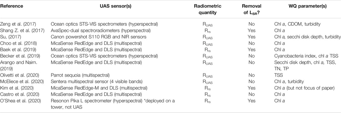
TABLE 1. Summary of existing UAS aquatic remote sensing literature including the UAS sensor(s) used, radiometric quantity studied (where R_rs represents UAS derived remote sensing reflectance and R_UAS represents UAS derived total reflectance), whether the study accounted for surface reflected radiance (L_SR), and the water quality parameter(s) derived.

Like all above-water optical measurements, UAS do not measure R_rs directly as the at-sensor total radiance (L_T, W m⁻² nm⁻¹ sr⁻¹) constitutes the sum of L_W and incident radiance reflected off the sea surface into the detector’s field of view, herein referred to as surface-reflected radiance (L_SR). L_W is radiance that emanates from the water and contains a spectral shape and magnitude governed by optically active water constituents interacting with downwelling irradiance, while L_SR is independent of water constituents and is instead governed by a given sea-state surface reflecting light; a familiar example is sun glint. Here we define UAS total reflectance (R_UAS) as:

$R_{UAS}\left(\text{θ},\Phi ,\text{ λ}\right)=\frac{L_T\left(\text{θ},\Phi ,\text{ λ}\right)}{E_d\left(\text{λ}\right)}(2)$

where

$L_T\left(\text{θ},\Phi ,\text{ λ}\right)= L_W\left(\text{θ},\Phi ,\text{ λ}\right)+ L_{SR}\left(\text{θ},\Phi ,\text{ λ}\right)(3)$

As UAS measurements are typically performed close to the surface (e.g. United States Federal Aviation Administration's maximum allowable altitude of 122 m), atmospheric measurement effects are routinely assumed to be negligible and ignored (Zeng et al., 2017; Schneider-Zapp et al., 2019). Indeed, this is a key advantage of UAS imagery as atmospheric effects over coastal environments can introduce significant uncertainty in satellite-based measurements (Gordon and Clark, 1980). However, failure to accurately account for L_SR can significantly influence R_rs, resulting in inaccurate water quality estimates once algorithms are applied (Su, 2017; Zeng et al., 2017).

The objective of this paper is to evaluate the efficacy of methods that remove L_SR from total UAS radiance measurements in order to derive more accurate remotely sensed retrievals of scientifically valuable in-water constituents. UAS derived radiometric measurements are evaluated against in situ hyperspectral R_rs measurements to determine the best performing method of estimating and removing surface reflected light and derived water quality estimates.

Background/Theory

If a water surface was perfectly flat, incident light would reflect specularly and could be measured with known viewing geometries. This specular reflection of a level surface is known as the Fresnel reflection; however, most water bodies are not flat as winds and currents create tilting surface wave facets. Due to differing orientation of wave facets reflecting radiance from different parts of the sky, L_SR can vary widely within a single image. A common approach to model L_SR is to express it as the product of sky radiance (L_sky, W m⁻² nm⁻¹ sr⁻¹) and ⍴, the effective sea-surface reflectance of the wave facet (Mobley, 1999 ; Lee et al., 2010):

$L_{SR}\left(\text{θ},\Phi ,\text{ λ}\right)= \rho \left(\text{θ},\Phi ,\text{ λ}\right)\ast L_{sky}\left(\text{θ},\Phi ,\text{ λ}\right)(4)$

Rearranging Eqs. 3 Eqs. 4, ⍴ can be derived by:

$\rho \left(\text{θ},\Phi ,\text{ λ}\right)=\frac{L_T\left(\text{θ},\Phi ,\text{ λ}\right)- L_w\left(\text{θ},\Phi ,\text{ λ}\right) }{L_{sky}\left(\text{θ},\Phi ,\text{ λ}\right)}(5)$

Given measurements of L_sky, an accurate determination of ⍴ is critical to derive R_rs by:

$R_{rs}\left(\text{θ},\Phi ,\text{ λ}\right)=R_{UAS}\left(\text{θ},\Phi ,\text{ λ}\right)-\frac{L_{sky}\left(\text{θ},\Phi ,\text{ λ}\right)\ast \rho \left(\text{θ},\Phi ,\text{ λ}\right) }{E_d\left(\text{λ}\right)}(6)$

Methods using the statistics of the sea surface, for a given wind vector, can be used to predict ⍴; tabulated values have been derived from numerical simulations with modelled sea surfaces, Cox and Munk wave states (wind), and viewing geometries (Cox and Munk, 1954; Mobley, 1999; Mobley, 2015). Mobley (1999) provides the recommendation of collecting radiance measurements at viewing directions of θ = 40° from nadir and ɸ = 135° from the sun to minimize the effects of sun glint and nonuniform sky radiance with a ⍴ value of 0.028. The suggested viewing geometries and ⍴ value from Mobley (1999) have been used to estimate and remove L_SR in UAS remote sensing studies (Ruddick et al., 2006; Shang S. et al., 2017; Baek et al., 2019; Kim et al., 2020). However, more recent studies have shown that ⍴ can be spectrally dependent due to the degree of sky polarization and the ratio of diffuse to direct light; assuming a spectally constant ⍴ in a roughened sea surface with multi-angular wave facets can lead to erroneous estimates of L_SR (Lee et al., 2010; Mobley, 2015). Lee et al. (2010) proposed a spectral optimization approach using spectral inherent optical properties to model R_rs, which has been applied in UAS remote sensing studies (O’Shea et al., 2020).

An alternative method to remove L_SR relies on the so-called dark pixel assumption that assumes L_W in the NIR is negligible due to strong absorption of water. Where this assumption holds, at-sensor radiance measured in the NIR is solely L_SR (Gordon and Wang, 1994; Siegel et al., 2000) and allows ⍴ to be calculated if L_sky is known. Studies have used this assumption to estimate and remove L_SR; however, the assumption tends to fail in more turbid waters where high concentrations of particles enhance backscattering and L_W in the NIR (Siegel et al., 2000; Lavender et al., 2005). Other novel image-processing techniques such as nonlocal mean filtering and a matching pixel by pixel algorithm have been proposed to reduce the effects of L_SR variation from UAS imagery; however, these region-specific methods exhibit some limitations for applications in other water bodies (Su, 2017; Totsuka et al., 2019).

Methods

Study Area

This study was conducted in the Choptank River, a major tributary of the Chesapeake Bay (United States). The 1,756 km² coastal plain watershed is dominated by agriculture and forest with a relatively low population density, transitions from non-tidal, freshwater reaches to a brackish, tidal mouth, and is eutrophic (Fisher et al., 2021). Data from eight stations located downriver and extending from the mouth of the Choptank River were collected on September 16, 2020 with a relatively clear sky, data from eight stations located up river were collected on October 1, 2020 with varying cloud cover, and data from thirteen stations located in between the downriver and upriver stations were collected on October 22, 2020 with a clear sky (Figure 1).

FIGURE 1

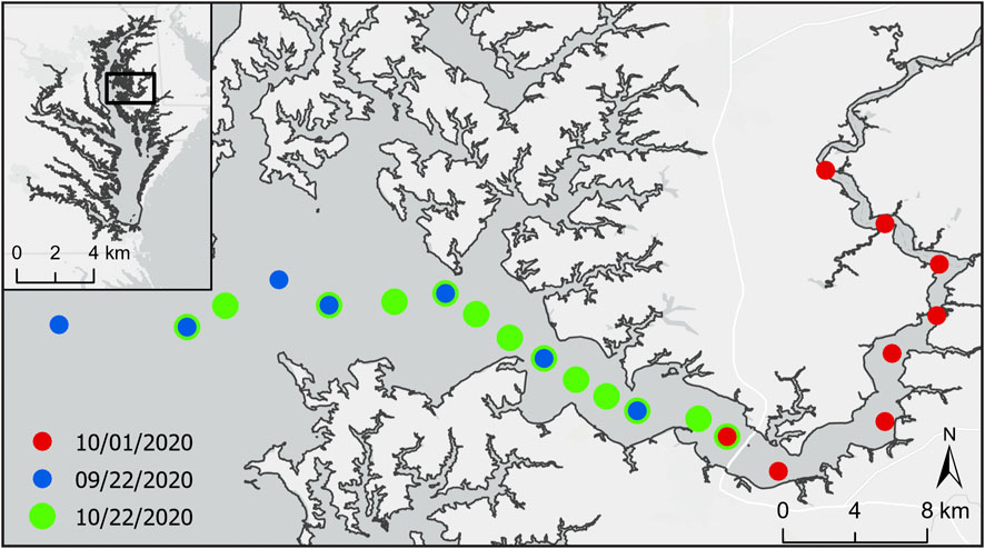
FIGURE 1. Location of Choptank River (38.63 N, −76.33 W) in Chesapeake Bay, Maryland, United States and locations of stations where data was collected.

In situ R_rs

At each station, a set of hyperspectral radiometers (TriOS RAMSES; Rastede DE) deployed on a float provided in situ R_rs measurements at every station. The float held a downwelling irradiance sensor (E_d) and an inverted radiance sensor (L_w) positioned above the surface water and with a small black plastic cone that extended just below the surface to block L_SR (i.e. light blocking technique, Ahn et al., 1999; Lee et al., 2019). The TriOS radiometers collect 256 wavelength bands at 3.3 nm intervals within the 320–950 nm range. All in situ hyperspectral measurements were interpolated at 1 nm intervals. In order to compare these measurements to the UAS, spectral response functions (SRFs) of the five MicaSense wavebands were applied to the in situ hyperspectral R_rs data (Figure 2).

FIGURE 2

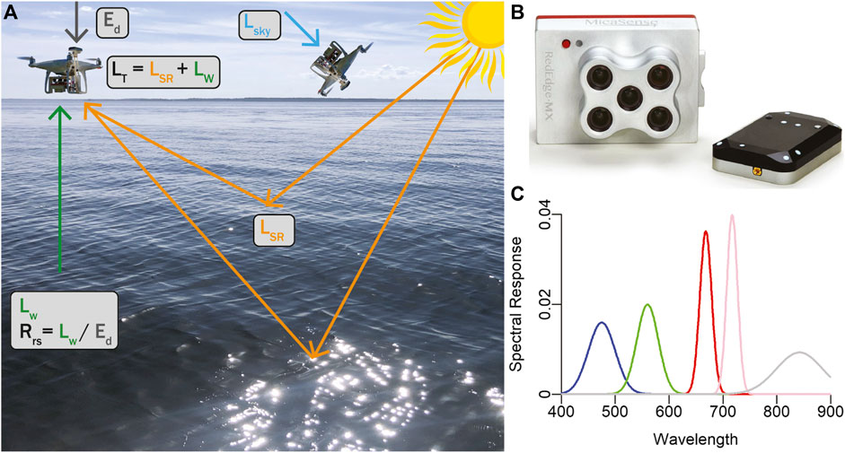
FIGURE 2. (A) MicaSense RedEdge-MX multispectral sensor and downwelling light sensor (DLS) collects total radiance (L_T) (sum of water-leaving radiance, L_w and surface reflected radiance, L_SR) and downwelling irradiance (E_d) measurements while in a low altitude flight. Sky radiance (L_sky) is collected by positioning the sensor at 40° angle from zenith away from sun. (B) MicaSense RedEdge-MX multispectral sensor and DLS collects L_T and E_d in five wavebands: red, green, blue, red-edge, near-infrared. (C) Approximate spectral response functions of MicaSense RedEdge-MX sensor.

In situ Water Quality Data

At each station, surface water grab samples were collected to measure chlorophyll a and total suspended solids (TSS) concentrations. Chlorophyll a concentration was measured in duplicate following EPA method 445.0 (Arar and Collins, 1997). Briefly, 100 ml of water from each station was filtered on 47 mm GF/F filters, immersed in 20 ml of 90% acetone and placed in a dark freezer for 24 h. Chlorophyll a fluorescence was measured on 5 ml of extract using a fluorometer (Turner 10 AU Fluorometer, San Jose CA) calibrated against chlorophyll a pigment standards (DHI, Horsholm DK) before and after acidification with 0.1 ml of 6 N hydrochloric acid. TSS was measured using a gravimetric analysis (American Public Health Association (APHA), 1995). 350 ml of water from each station was filtered using pre-weighed and combusted (450°C) GF/F filters and placed into a 105°C drying oven for at least 2 h. Filters were reweighed and the concentration was calculated by TSS (mg/L) = W_post(g) - W_combust(g) x 1,000/V(L).

Multispectral Sensor: MicaSense RedEdge-MX Sensor

The MicaSense RedEdge-MX sensor (MicaSense, Seattle, Washington, United States) is a 8.7 × 5.9 × 4.5 cm multispectral camera capable of capturing five simultaneous bands on the electromagnetic spectrum in 12 bit radiometric resolution: blue (475 nm center, 32 nm bandwidth), green (560 nm center, 27 nm bandwidth), red (668 nm center, 14 nm bandwidth), red edge (717 nm center, 12 nm bandwidth), and NIR (842 nm center, 57 nm bandwidth). The sensor has up to one capture per second, a 47.2° field of view with a spatial resolution of 8 cm per pixel at 120 m altitude. The sensor was mounted on a DJI Phantom four Pro UAS using a 10° 3D-printed mount which resulted in a direct nadir viewing angle while in flight (Figure 2). The sensor also includes a downwelling light sensor (DLS) which measures E_d in the same spectral wavebands during in-flight image captures. The DLS measures light incident on a diffuser, providing a downwelling hemispherical irradiance measurement (Mamaghani and Salvaggio, 2019). The DLS was mounted above the UAS to eliminate shading and collected incident light at a 0° zenith angle. Images were collected at an average flight altitude of 70 m which resulted in 0.02 m pixel resolution (923 × 1219).

At each station, measurements of L_T, L_sky, and E_d were collected by the MicaSense RedEdge-MX multispectral sensor and DLS. First, measurements of L_sky were collected by positioning the camera 40° from zenith with an approximate azimuthal viewing direction of 135° and taking several image captures (Figure 2). L_sky at each waveband was computed as the grand mean of all station-specific measurements. Next, the UAS was manually flown and images were automatically captured every 2 s. The MicaSense multispectral sensor has a built-in global positioning system (GPS) and inertial measurement unit (IMU) which recorded the positioning (latitude, longitude, altitude) and orientation (yaw, pitch, roll) of each image capture. Thirty image captures taken at the highest altitude from each station were used in subsequent analyses. This information along with solar elevation, image size, and coordinated universal time (UTC) time, were recorded in the metadata of each image capture.

Pre-Processing

Data collected by the multispectral sensor were radiometrically calibrated using a Python workflow provided by MicaSense¹. The process of converting raw pixel values (digital number, DN) into total spectral radiance (L_T) values with units of W/m/sr/nm is given in Eq 7:

$L_T=V\left(x,y\right)\ast \frac{a_1}{g}\ast \frac{DN - D{N}_{BL}}{t_e + a_{2}y- a_3{t}_{e}y}(7)$

The radiometric calibration compensates for dark pixel subtraction (DN_BL), sensor gain (g), exposure settings (t_e), and lens vignette effects (V(x,y)). Coefficients a₁, a₂, and a₃ are radiometric calibration coefficients and x,y is the pixel column and row number, respectively. Lens distortion effects, such as band-to-band image alignment, were removed from image captures by an unwarping procedure and wavebands were aligned to form a stacked TIFF for each image set.

A filtering procedure was applied to all images to remove specular sun glint and instances of the boat when it was present in the image. Studies have suggested filtering out high total radiance values, or instances of specular sun glint, before removing L_SR from L_T (Hooker et al., 2002). Specular sun glint arises when direct sunlight reflects off of a wave facet or surface at the viewing angle of the sensor. Sun glint pixels were masked using an empirical upper limit of R_UAS measurements in the NIR, and this mask was then propagated to pixels at all other wavebands. Specifically, in situ measurements and values from radiative transfer model simulations (see methods below) were used in Eq. 8 to solve for an upper limit of R_UAS(NIR) and pixels with values greater than this upper limit were masked in each waveband.

$R_{UAS}\left(NIR\right)= R_{rs}\left(NIR\right)+ \mathrm{\rho }\left(\text{NIR}\right)\ast \frac{L_{sky}}{E_d}(8)$

Where R_rs(NIR) = 0.005 is based on in situ measurements in this study and consistent with other turbid waters (Tzortziou et al., 2006), ⍴(NIR) varied depending on station, and L_sky/E_d = 0.39 is derived from radiative transfer model simulations (HydroLight v6.0, Numerical Optics Ltd., United Kingdom). A lower limit of R_UAS(green) = 0.007 was used to mask out the dark canopy of the boat when present in images.

Removal of Surface Reflected Light (L_SR)

At each station, L_SR was estimated using one of four different methods to ultimately derive R_rs following Eq. 6. These methods are provided below, and herein referred to as “⍴_LUT,” “NIR = 0,” “NIR > 0” and “Deglinting.” Resultant UAS R_rs estimates were then compared to paired in situ R_rs data across stations and wavebands. Statistical evaluations to assess the relationship included root mean square error (RMSE), relative root mean squared error (RRMSE), coefficient of determination (R²), and p-values.

⍴_LUT. The ⍴_LUT method follows from Mobley (1999) and involved developing a look-up table (LUT) of ⍴ values using HydroLight simulations. HydroLight is a numerical model that solves the radiative transfer equation to compute the radiance distribution within and at the surface of a water body. Inputs include absorbing and scattering properties of a water body, the nature of the wind-blown sea surface (Cox-Munk sea surface slopes), and the sun and sky radiance incident on the sea surface (Mobley, 1999). Outputs include the full radiance distribution, including an effective ⍴ value for a range of geometries and wavelengths. Batch HydroLight runs incorporating varying solar zenith angles (0, 10, 20, 30, 40, 50, 60°), wind speeds (0, 2, 4, 6, 8 m/s), and fractional cloud cover (0, 0.2, 0.4, 0.6, 0.8, 1%) were used to develop a multidimensional look-up table of ⍴ values that correspond to a nadir viewing angle (Figure 3). HydroLight returned spectrally explicit ⍴(θ, ɸ, λ) values and MicaSense SRFs were applied to ⍴(θ, ɸ, λ) for each waveband. ⍴(θ, ɸ, λ) values were obtained for each station according to the solar zenith angles obtained from MicaSense metadata, wind speed was collected from the Global Forecast System², and cloud cover was determined by the L_sky images. Data in this study were collected at solar zenith angles ranging from 36.5 to 58.6°, wind speeds ranged from 1.1 to 3.1 m/s and cloud cover ranged from 0 to 60%.

FIGURE 3

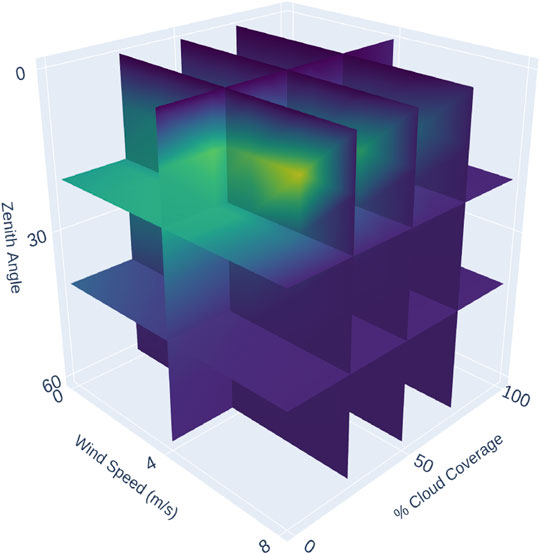
FIGURE 3. Visualization of the three-dimensional ⍴ look-up table derived from HydroLight simulations with varying solar zenith angles, wind speed (m/s), and cloud cover (%) corresponding to a nadir viewing angle.

NIR = 0. L_SR was also estimated using a pixel based dark pixel assumption to derive ⍴. Assuming R_rs(NIR) equals 0, Eq. 6 can be rearranged to solve for ⍴ (Eqs. 9 and 10). This ⍴ value is used to calculate R_rs across all wavebands (Eq. 11).

$0=L_T\left(NIR\right)-L_{sky}\left(NIR\right)\ast \mathrm{\rho }(9)$

$\mathrm{\rho }=L_T\left(NIR\right)/L_{sky}\left(NIR\right)(10)$

$R_{rs}\left(\text{θ},\Phi ,\text{ λ}\right)=R_{UAS}\left(\text{θ},\Phi ,\text{ λ}\right)-\frac{L_{sky}\left(\text{θ},\Phi ,\text{ λ}\right)\ast (L_T\left(NIR\right)/L_{sky}\left(NIR\right)) }{E_d\left(\text{λ}\right)}(11)$

NIR > 0. Since the dark pixel assumption is invalid in turbid waters including the Chesapeake Bay (Siegel et al., 2000) an alternative pixel based approach was developed to instead estimate a baseline R_rs(NIR). Specifically, R_rs(NIR) was estimated empirically by a nonlinear regression using in situ R_rs(NIR) and R_UAS data (Figure 4). The ratio of R_UAS(blue)/R_UAS(rededge) led to the most robust predictions of R_rs(NIR) using Eq 12:

$R_{rs}\left(\text{θ},\Phi ,\text{ λ}\right)=0.025e^{-5.469\ast R_{UAS}\left(blue\right)/R_{UAS}(red edge) }+0.00013(12)$

FIGURE 4

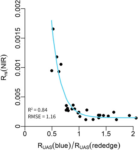
FIGURE 4. Nonlinear relationship between a blue (475 nm) to red edge (717 nm) ratio of total UAS reflectance to in situ R_rs in the NIR band (842 nm). An exponential model was used to estimate UAS derived R_rs(NIR) baseline in order to estimate L_SR.

Conceptually, this relationship makes sense because with increasing particle concentrations, water becomes less blue and R_rs(NIR) increases.

“Deglinting.” L_SR was also estimated following the “deglinting” methods of Hochberg et al. (2003) and Hedley et al. (2005). For each station, a minimum NIR value was determined by finding the lowest 10% of R_UAS(NIR) across all images. For each band, a linear regression was made between all R_UAS(NIR) and R_UAS(visible) values and the slope (b_i) was determined. Each pixel was corrected by subtracting the product of b_i and the NIR brightness of the pixel (Hedley et al., 2005):

$R_{rs}\left(i\right)= R_{UAS}\left(i\right)-b_i(R_{UAS}\left(NIR\right)-\min \left(R_{UAS}\left(NIR)\right)\right)(13)$

Water Quality Retrievals

R_rs values from each L_SR removal method were compared against in situ chlorophyll a and TSS data (n = 28) using multiple linear regressions. The best performing model (highest R² and lowest RMSE, RRMSE, p-values) was used in a stepwise model selection by Akaike information criterion (AIC, “stepAIC” in R). The AIC stepwise regression iteratively added and removed wavelengths in order to determine the combination of data that resulted in the best performing model with low prediction error, while taking into account model simplicity. R_rs values were used as input into optical algorithms derived from the best performing multiple linear regressions and mean chlorophyll a and TSS concentration at each station was obtained by averaging values across all images. The resulting arrays were georeferenced using the Python libraries “CameraTransform” (Gerum et al., 2019) and “Rasterio” using archived metadata including latitude, longitude, image width, image height to position the images accurately in a known coordinate system (WGS84). Georeferenced arrays were exported as individual TIFFs and mapped using ArcGIS Pro (ESRI Inc. Redlands, CA, United States).

Results

In situ Data

Chlorophyll a concentration ranged from 5.19 to 53.30 ug/L with an average of 17.13 ± 10.96 ug/L. TSS concentration ranged from 19.94 mg/L to 39.69 mg/L with an average of 28.25 ± 5.21 mg/L. In general, in situ R_rs spectra were representative of a eutrophic system (Figure 5, Gitelson et al., 2007; Spyrakos et al., 2018). Due to absorption of chromophoric dissolved organic matter (CDOM) and chlorophyll a in lower wavelengths, R_rs is low in the blue region with a distinct peak in the green region (∼550 nm). A secondary peak in the red region (∼700 nm) corresponds to chlorophyll fluorescence emission (Spyrakos et al., 2018). Overall, spectra collected from upriver stations on 10/01/20 were larger in magnitude and contained a tertiary peak in the NIR region (∼800 nm).

FIGURE 5

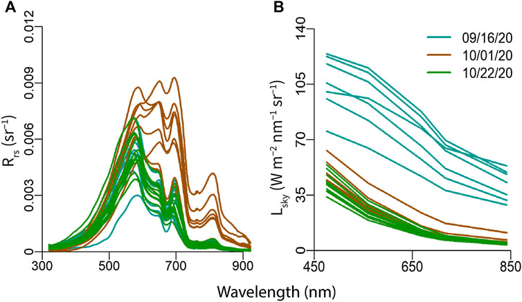
FIGURE 5. (A)In situ remote sensing reflectance (R_rs) spectra collected with hyperspectral TriOS radiometers and (B) Sky radiance (L_sky) spectra collected with MicaSense RedEdge-MX multispectral camera at stations along the Choptank River on 9/16/20 (blue), 10/01/20 (brown), and 10/22/20 (green).

Removal of Surface Reflected Light (L_SR)

UAS measurements of L_sky were approximately proportional to the fourth power of the wavelength (L_sky ≈ λ⁻⁴, Figure 5) and were used with estimations of ⍴ to calculate and remove L_SR from R_UAS measurements at each station. Figure 6 illustrates the initial masking and methods to remove L_SR using an individual UAS image taken in the green band. When L_SR was estimated using the ⍴ look-up table (⍴_LUT), R_rs values did not change much from R_UAS values; however, R_rs values using the pixel-based dark pixel assumptions (NIR = 0, NIR>0) and “deglinting” approach declined and became more homogenous across pixels (Figure 6).

FIGURE 6

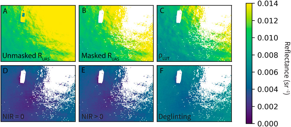
FIGURE 6. Example of an individual UAS image (green band) with different radiometric values: (A) R_UAS, (B) R_UAS with initial sun glint masking and (C–F) remote sensing reflectance (R_rs) using various methods to remove surface reflected light: (C) ⍴ look-up table (LUT) from HydroLight simulations, (D) Dark pixel assumption with NIR = 0, (E) Dark pixel assumption with NIR >0, (F) Deglingting methods following Hochberg et al. (2003).

UAS derived reflectance measurements from each L_SR removal method were plotted as spectra (Figure 7) and compared against in situ R_rs values (Figure 8). UAS reflectance spectra are similar in shape to in situ R_rs spectra and display a distinct peak in the green band (560 nm) and often a secondary peak in the red band (668 nm) corresponding to chlorophyll a reflectance and fluorescence, respectively (Figure 7). Spectra collected on the second sampling day (upriver sites) shift to longer wavelengths likely due to scattering of inorganic particles (Figure 7). R_UAS spectra are higher in magnitude and are overestimated when compared to in situ R_rs due to the inclusion of L_SR (R² = 0.55, RMSE = 0.004, p < 0.05). When L_SR is estimated using the ⍴_LUT, spectra are similar in shape to in situ spectra, but are higher in magnitude and overestimated compared to in situ measurements (R² = 0.85, RMSE = 0.003, p < 0.05). When L_SR is estimated with the dark pixel assumption (NIR = 0), R_rs spectra are lowest in magnitude, had the poorest fit to in situ data (R² = 0.18, RMSE = 0.004, p < 0.05), and produced negative R_rs values in the lower wavelengths. This is not surprising given that the in situ measurements in the NIR (Figure 5A) are not negligible which leads to an overestimation in L_SR. When L_SR is estimated using a basline NIR value (NIR>0), R_rs spectra are higher in magnitude with a lower error but still indicate negative values in the lower wavelengths, indicating L_SR was still slightly overestimated (R² = 0.50, RMSE = 0.002, p < 0.05). R_rs spectra with the “Deglinting” approach are similar in shape to in situ spectra but are slightly higher in magnitude (Figure 7). This approach contained the second highest correlation and lowest RMSE (R² = 0.65, RMSE = 0.002, p < 0.05), but still tended to overestimate R_rs values (Figure 8).

FIGURE 7

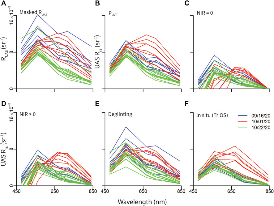
FIGURE 7. Total UAS reflectance (R_UAS) (A) and remote sensing reflectance (R_rs) spectra using various methods to remove surface reflected light: (B) ⍴ look-up table from HydroLight simulations, (C) Dark pixel assumption with NIR = 0, (D) Dark pixel assumption with NIR >0, (E) Deglinting methods following Hochberg et al. (2003), and (F)In situ R_rs spectra from TriOS sensors with MicaSense SRFs applied. Negative values are not shown in plots.

FIGURE 8

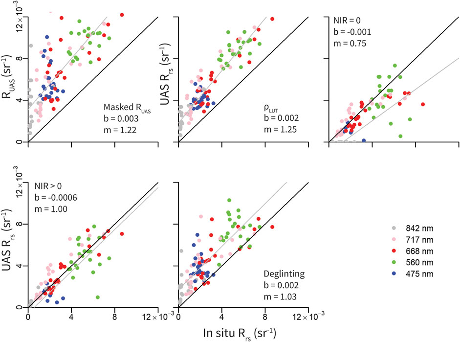
FIGURE 8. Comparison of UAS radiometry and in situ R_rs in all bands at each station (n = 28) using different methods to remove surface reflected light after initial sun glint masking. (A) Total UAS derived reflectance (R_UAS), (B) ⍴ look-up table from HydroLight simulations, (C) Dark pixel assumption with NIR = 0, (D) Dark pixel assumption with NIR >0, (E) Deglinting methods following Hochberg et al. (2003). Negative values are not shown in plots.

Water Quality Retrieval Algorithms

R_rs measurements with L_SR estimated using a baseline NIR value (NIR>0) performed best when compared to in situ chlorophyll a data (R² = 0.37, RMSE = 5.89, RRMSE = 37%, p < 0.05). A stepwise model selection by AIC demonstrated that the green, red edge, and NIR bands were most important in estimating chlorophyll a concentration (Figure 9, R² = 0.42, RMSE = 5.90, RRMSE = 37%, p < 0.05) and a remotely sensed chlorophyll a algorithm was determined as:

$\text{Chlorophyll a }\left(\text{ug/L}\right)=24{\text{.}02+\text{ R}}_{\text{rs}}\left(\text{560}\right)\text{ * }-4337{\text{.}88+\text{ R}}_{\text{rs}}\left(\text{717}\right)\text{ * }9639{\text{.}75+\text{ R}}_{\text{rs}}\left(\text{842}\right)\text{ * }-2922\text{.}80$

FIGURE 9

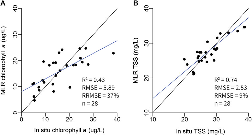
FIGURE 9. Comparison between in situ and modelled (A) chlorophyll a concentration and (B) TSS concentration from multiple linear regressions.

R_rs measurements with the “deglinting” technique performed best when compared to in situ TSS data (R² = 0.72, RMSE = 2.53, RRMSE = 9%, p < 0.05). A stepwise model selection by AIC demonstrated that the blue, red, red edge, and NIR bands were most important in estimating TSS concentration (Figure 9, R² = 0.73, RMSE = 2.53, RRMSE = 9%, p < 0.05) and a remotely sensed TSS algorithm was determined as:

$\text{TSS }\left(\text{mg/L}\right)=30{\text{.}57+\text{ R}}_{\text{rs}}\left(\text{475}\right)\text{ * }1364{\text{.}86+\text{ R}}_{\text{rs}}\left(\text{668}\right)\text{ * }-5255{\text{.}88+\text{ R}}_{\text{rs}}\left(\text{717}\right)\text{ * }2548{\text{.}08+\text{ R}}_{\text{rs}}\left(\text{842}\right)\text{ * }4579\text{.}36$

Algorithms were applied to respective UAS derived R_rs values and average chlorophyll a and TSS concentrations were mapped, along with mosaiced georeferenced TIFFs of individual image captures (Figure 10). Average chlorophyll a concentration tended to increase at upriver sites while average TSS concentrations were higher at downriver sites (Figure 10). This trend was also seen in the in situ data. Within the mosaic of individual TIFFs, slight variations in chlorophyll a and TSS concentration are visible (Figure 10).

FIGURE 10

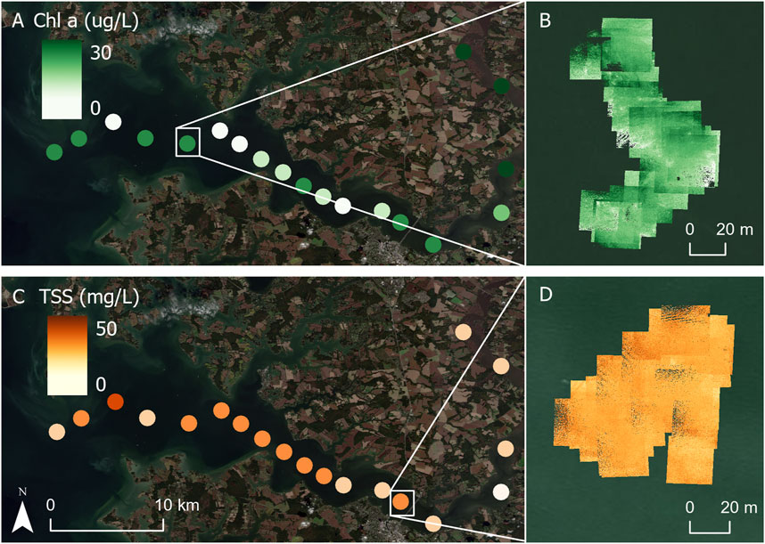
FIGURE 10. (A) Average chlorophyll a concentration across image captures (n = 30) at each station. (B) Example of mosaiced georeferenced TIFFs collected at one station with chlorophyll a algorithm applied. (C) Average TSS concentration across image captures (n = 30) at each station. (D) Example of mosaiced georeferenced TIFFs (n = 30) collected at one station with TSS algorithm applied.

Discussion

This study is one of the first to compare methods to remove surface reflected light from high resolution UAS multispectral measurements. An initial filtering procedure and four methods to remove L_SR were evaluated against in situ R_rs measurements. Water quality algorithm performance is compared to those found in the literature. Results have broad implications for improving UAS derived water quality measurements in coastal waters, but several aspects and caveats of this study merit additional discussion.

Performance of Methods to Remove Surface Reflected Light (L_SR)

Removing surface reflected light from the total radiance measured by a UAS ensures only water-leaving information is used as input into water quality retrievals. Initial filtering techniques successfully masked instances of specular sun glint and non-water objects (i.e. boat) in the UAS imagery using empirical upper and lower R_rs limits. This primary step ultimately improved final R_rs measurements and derived water quality products. While the magnitude of L_sky can impact L_SR, the spectral dependence (∼λ⁻⁴) is constrained and can be measured; therefore, the effective sea-surface reflectance of a wave facet (⍴) needs to be accounted for. Nonetheless, it is important to consider the impact of the varying absolute magnitude of L_sky and future work should analyze the effect of L_sky variability on UAS R_rs measurements.

The ⍴_LUT method utilized a ⍴ lookup table approach developed from HydroLight simulations where ⍴ values were obtained depending on the solar zenith angle, wind speed, and cloud cover at the time of UAS data collection. Mobley (1999) HydroLight simulations led to recommendations of specific sensor viewing angles with a corresponding constant ⍴ value to reduce effects of L_SR; however, most consumer grade UAS sensors and mounts do not have the ability to change viewing angles and are fixed at a nadir viewing angle. Therefore, the ⍴ values in the look-up table correspond to nadir viewing angles. This method resulted in UAS R_rs values that were generally greater than in situ R_rs values, indicating L_SR was underestimated. This can most likely be attributed to a constant ⍴ value that was used to estimate L_SR across all pixels in each image, which averaged out the multifaceted characteristic of a water surface.

The NIR = 0 and NIR >0 methods took advantage of the NIR waveband on the multispectral sensor and incorporated aspects of the dark pixel assumption which allowed L_SR to be removed from visible wavelengths by assuming that 1) a NIR signal is composed of L_SR and/or a spatially homogeneous NIR component in the water and 2) the amount of L_SR in the NIR band is linearly related to the amount of L_SR in the visible bands (Mobley, 1999; Siegel et al., 2000). Unlike the ⍴LUT method that applies a single value to an entire image, the dark pixel assumption approaches estimate L_SR on a per pixel basis which decreases resultant R_rs variability (Figures 6, 8). When NIR was assumed to be entirely negligible, calculated R_rs values were generally lower compared to in situ R_rs which can be attributed to an enhancement of NIR due to the presence of scattering inorganic particles in turbid waters. Thus, when a baseline NIR value was estimated, the method performed better (higher R², lower RMSE and RRMSE); however, negative R_rs values in the lower wavelengths indicated L_SR was still likely overestimated at some stations.

The “deglinting” method, modelled off a glint removal algorithm introduced by Hochberg et al. (2003), and later Hedley et al. (2005), calculated a constant ‘ambient’ NIR brightness level which was removed from all pixels in all wavelengths. This approach resulted in UAS R_rs measurements slightly overestimated compared to in situ values but produced the highest R² and lowest RMSE of all methods. This method was applied by averaging pixel values across all thirty images collected at each station and is likely to perform better when applied on individual images.

The ⍴_LUT method uses ⍴ values that are based on probability distributions of sea surface slopes which are related to the scale of satellite pixel resolution (100–1000 m) (Cox and Munk, 1954). For images with much higher pixel resolution ( >1–10 m), statistical assumptions about the surface of water composed of many reflecting facets are less likely to hold (Kay et al., 2009). Therefore, to collect accurate water-leaving reflectance measurements from high resolution UAS imagery, it is recommended to use a pixel-based approach exploiting the high absorption of water at NIR wavelengths to estimate and remove L_SR. If a baseline NIR measurement can be retrieved, the dark pixel assumption should be used to remove L_SR. Otherwise, the ‘deglinting’ methods following Hochberg et al. (2003) and Hedley et al. (2005) are recommended. In open ocean waters without a strong influence of optically active properties, a pixel-based approach assuming NIR is negligible is expected to perform well.

It is important to note a potential caveat to the L_SR method evaluation. In this study, in situ R_rs measurements were provided by hyperspectral radiometers with a skylight blocking approach (Ahn et al., 1999; Lee et al., 2019). This approach consists of attaching an open-ended apparatus, or tube, to the front of a downward looking radiance radiometer and lowering it a few centimeters into the water, blocking surface-reflected light and allowing for a direct measurement of L_W. It is important to note that measurements from this technique are subject to instrument self-shading, which is a function of the water’s optical properties, sun elevation, and the size of the skylight-blocking cone (Zhang et al., 2017; Lee et al., 2019). Zhang et al. (2017) estimated that self-shading accounts for approximately 1–20% error under most water properties and solar positions. Methods to correct for this self-shading have been derived (Zhang et al., 2017; Yu et al., 2021) and if applied, have the potential to improve relationships with UAS R_rs measurements.

Performance of Water Quality Algorithms

Performance of the multiple linear regressions developed in this study were compared to existing chlorophyll a and TSS algorithms designed for coastal waters to determine if UAS measurements can produce accuracy within the range of other water quality algorithms. Performance of the UAS derived chlorophyll a multiple linear regression (R² = 0.43, RRMSE = 37%) is comparable to other chlorophyll a algorithms found in the literature (Ruddick et al., 2001; Gons et al., 2002; Gitelson et al., 2007). A three-band chlorophyll algorithm calibrated using a variety of coastal waters, including the Choptank River, resulted in a RRMSE of 51.9% (Gitelson et al., 2007), a two-band algorithm (red/NIR) with adaptive optimization in the second band calibrated with measurements from the North Sea and Lake Ijless, Netherlands resulted in a RRMSE of 37% (Ruddick et al., 2001), and a two-band algorithm (red/NIR) designed for the Medium Resolution Imaging Spectrometer (MERIS) satellite sensor and calibrated using a variety of coastal and inland waters including Lake IJssel (Netherlands), the Chinese Lake Tau Hu, and the Hudson/Raritan Estuary (New York/New Jersey) resulted in a standard error of 9.2 ug/L (Gons et al., 2002). Performance of the UAS derived TSS multiple linear regression (R² = 0.73, RMSE = 2.53, RRMSE = 9%) is also comparable to existing TSS algorithms found in the literature (Nechad et al., 2010; Novoa et al., 2017). Algorithms including a single-band (NIR) second-order polynomial and single-band (red/green) linear models calibrated with measurements from the Gironde Estuary, France resulted in RRMSE values ranging from of 9.11–16.41% (Novoa et al., 2017) and a non-linear regression calibrated with measurements from the Southern North Sea resulted in RRMSE values less than 30% (Nechad et al., 2010). Future work will include improving water quality algorithms.

UAS Sensor Considerations

The innovative use of UAS technology for environmental research is a relatively new field and researchers are only beginning to understand and alleviate the various methodological and sensor performance challenges. Sensors degrade over time from use and environmental conditions which can impact the accuracy of the data being collected. The most recent MicaSense model, the MicaSense RedEdge-MX, is integrated with low-cost, image-frame complementary metal-oxide semiconductor (CMOS) sensors, which compared to typical charged-coupled device (CCD) sensors, tend to generate more noise and have lower sensitivity levels (Mamaghani and Savaggio, 2019). In the present study, raw values were radiometrically calibrated using a workflow¹ provided by Micasense which implements default metadata parameters that remain the same unless a new factory calibration is performed. Due to sensor degradation, these values are likely to gradually decline over time, lessening the accuracy of the radiometric calibration processing (Mamaghani and Savaggio, 2019). Studies have improved sensor performance by performing vicarious radiometric calibration using ground targets and panels with known radiometric accuracy, calibrating sensors using National Institute of Standards (NIST)-traceable equipment in a laboratory, and developing look-up tables for correction factors to update calibration parameters (Del Pozo et al., 2014; Mamaghani and Salvaggio, 2019; Cao et al., 2020). Baek et al. (2020) conducted an assessment on radiometric accuracy for the MicaSense RedEdge-MX sensor by comparing data to hyperspectral sensors with NIST-traceable calibration (TriOS RAMSES) and showed that MicaSense RedEdge-MX radiance is approximately 5–16% lower, and irradiance is approximately 1–20% lower, depending on wavelength (Baek et al., 2020). The radiometric accuracy of a new or recently/vicariously calibrated UAS sensor should meet the required radiometric accuracy of 5% that is expected with ocean color satellites (McClain et al., 1992).

Precise registration of multispectral bands within a UAS image capture is also important to derive accurate spectral radiometric values across pixels. Sources of misregistration include a difference in the lens location for each band, image acquisition times, and exposure times which can all influence R_rs and resulting water quality variables (Kim et al., 2020). In the present study, images collected in each band were registered using MicaSense’s default alignment function¹. This three step process unwarps images using built-in lens calibration, determines a transformation to align each band to a common band, and crops pixels which do not overlap in all bands. Although this method seemed to perform well in this study; it is acknowledged that this type of band registration can perform poorly with images of locational errors, such as moving water, and can produce noise even after removing surface reflected light (Kim et al., 2020). Kim et al. (2020) developed a novel morphological band registration technique designed for high resolution water quality analysis which effectively removes misregistration noise and improves the accuracy of R_rs. Future aquatic UAS remote sensing work should consider adapting this technique to improve UAS remotely sensed retrievals over water.

Caveats and Considerations

Many UAS aquatic remote sensing studies use Structure-from-Motion (SfM) photogrammetric techniques to stitch individual UAS images into ortho- and georectified mosaics (Arango and Nairn, 2019; Castro et al., 2020; McEliece et al., 2020; Olivetti et al., 2020). This approach applies matching key points from overlapping UAS imagery in camera pose estimation algorithms to resolve 3D camera location and scene geometry (Westoby et al., 2012; Arango et al., 2020). Commonly used software (e.g. Pix4D) provide workflows that radiometrically calibrate, georeference, and stitch individual UAS images using a weighted average approach to create at-sensor reflectance 2D orthomosaics (Olivetti et al., 2020). L_SR removal methods and water quality algorithms can be directly applied to reflectance orthomosaics to effectively derive water quality products of an entire water body. However, current photogrammetry techniques are not capable of stitching UAS images captured over large bodies of water due to a lack of key points in images of homogenous water surfaces (Arango et al., 2020). Orthomosaics of smaller water bodies or rivers can be created if UAS images contain enough surrounding land features containing keypoints that the photogrammetry software can use to successfully stitch the images containing water. This can be accomplished by increasing flight altitude, with the trade-off of lower spatial resolution. Alternative methods include a statistical interpolation method; however interpolated reflectance values can be imprecise when compared to true reflectance values (Arango et al., 2020).

Management Implications and Future Research

Water quality monitoring is important for tracking water quality trends, identifying and mitigating pollution sources, and discerning potential human health risks. Traditional in situ based methods of sampling at discrete stations can be expensive due to high costs for boat time and analysis and can also potentially omit important water quality phenomena. Traditional satellite remote sensing can capture variability throughout time and space; however, limitations including the presence of clouds, atmospheric effects, land adjacency effects, and spatial resolution can hinder periodic monitoring (Shi and Wang, 2009; Becker et al., 2019). UAS fill an operational gap between in situ and satellite remote sensing methods. While the current available commercial multispectral UAS sensor technology is geared toward terrestrial applications, mostly precision agriculture, the spectral bands have been useful in retrieving water quality parameters in aquatic water bodies (Choo et al., 2018; Arango and Nairn, 2019; Baek et al., 2019; Castro et al., 2020; Olivetti et al., 2020). A UAS sensor package designed for aquatic environments would undoubtedly improve remotely sensed retrievals and water quality measurements.

Since UAS are deployed at a low altitude, atmospheric corrections and remedies to the land adjacency effect are eliminated. UAS are rapidly deployable and can provide the spatial and temporal variability required for useful water quality monitoring in a dynamic and rapidly evolving environment. UAS can enhance fine-scale physical oceanography research by resolving small-scale phenomena and physical processes such as patchy algal blooms, frontal structures, and turbulence characteristics (Figure 11, Shang Z. et al., 2017; Osadchiev et al., 2020). UAS remotely sensed water quality retrievals will also likely improve with the development of lightweight, off-the-shelf hyperspectral sensors, allowing for higher spatial and spectral resolution to better distinguish optical properties of the water (Shang S. et al., 2017; O’Shea et al., 2020).

FIGURE 11

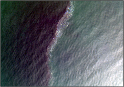
FIGURE 11. Frontal process observed in UAS RGB imagery collected in the Choptank River, Maryland, United States with MicaSense RedEdge-MX multispectral camera.

Future research in turbid coastal waters may benefit from sensor packages that use longer wavelengths (e.g. shortwave infrared, SWIR). SWIR wavelengths have shown to be more effective in satellite atmospheric correction techniques in turbid waters due to the stronger water absorption relative to NIR (Shi and Wang, 2009). This will be advantageous for removing L_SR and will improve R_rs retrievals in coastal, turbid waters. Future research could also consider combining UAS radiometry with photogrammetry computer vision to estimate L_SR. Schneider-Zapp et al. (2019) developed a method to estimate a hemispherical-directional reflectance factor (HDRF) from multi-angular UAS measurements. From a combination of photogrammetry and radiometry, a precise estimation of the downwelling light sensor position and orientation can be used to derive a multi-angular reflectance factor, which has the potential to significantly improve estimates of the multifaceted aspect of L_SR. An alternative approach to reduce L_SR is installing additional hardware to a UAS sensor. O’Shea et al. (2020) tested a hardware-based vertical polarizer on a hyperspectral spectrometer which effectively blocked horizontally polarized reflected skylight. This relatively simple approach could be an attractive solution to researchers and managers who are interested in applying a single algorithm to R_rs values to derive water quality parameters and should be further investigated.

Conclusion

UAS-based applications of multispectral or hyperspectral remote sensing in aquatic remote sensing have the potential to effectively fill current observation gaps in aquatic remote sensing and provide critical information needed for water quality forecasting, ecosystem monitoring, and ultimately climate change research. While atmospheric effects can usually be ignored in low altitude UAS flights, the effect of sun glint and surface reflected light should be accounted for in order to obtain the highest accuracy of water quality data. The inclusion of surface reflected light can lead to an overestimation of R_rs and remotely sensed water quality retrievals. This study presents a comparison of four approaches to remove sun glint and surface reflected light that can be applied to UAS remote sensing to derive water quality parameters such as chlorophyll a and TSS concentration. Overall, the performance of the MicaSense RedEdge-MX multispectral sensor appears sufficient for providing high resolution water quality estimates of coastal water bodies when surface reflected light is removed. Of the four approaches examined, a pixel-based deglinting procedure utilizing the brightness of the NIR band performed best when compared to in situ R_rs measurements. This method also led to the best estimates of TSS while a pixel-based approach utilizing an ambient NIR signal to estimate and remove surface reflected light led to the best estimates of chlorophyll a concentration. Future work will include improving algorithms for water quality parameters. Future research should also consider the effects of sensor calibration and the residual misregistration between bands of a UAS multispectral camera.

Data Availability Statement

The raw data supporting the conclusions of this article will be made available by the authors, without undue reservation.

Author Contributions

Both AW and GS contributed to the development, planning, and data collection of the study as well as the data analysis, interpretation, and writing of the manuscript.

Funding

AW received support from Maryland Sea Grant under award NA18OAR4170070, SA75281900-J from the National Oceanic and Atmospheric Administration, U.S. Department of Commerce and from the Mid-Shore Chapter of the Izaak Walton League. Equipment and parts were funded by Horn Point Laboratory.

Conflict of Interest

The authors declare that the research was conducted in the absence of any commercial or financial relationships that could be construed as a potential conflict of interest.

Acknowledgments

We thank the Choptank RiverKeeper, Matt Pluta from ShoreRivers for boat time during his routine water quality monitoring. Thank you to Ph.D. candidate Patrick Gray from the Duke Marine Robotics and Remote Sensing Lab for guidance and supportive conversations throughout this study.

Abbreviations

DLS, downwelling light sensor; E_d, downwelling irradiance; L, spectral radiance; L_SR, surface-reflected radiance; L_sky, sky radiance; LUT, lookup table; L_T, total radiance; L_W, water leaving radiance; NIR, near infrared; R_rs, remote sensing reflectance; R_UAS, UAS total reflectance; UAS, unoccupied aircraft system; ⍴, effective sea-surface reflectance of wave facet

Footnotes

¹MicaSense RedEdge Image Processing Tutorials. Retrieved online at https://github.com/micasense/imageprocessing.

²Wind speed data was retrieved from https://earth.nullschool.net/about.html.

References

Ahn, Y. H., Ryu, J. H., and Moon, J. E. (1999). Development of Redtide & Water Turbidity Algorithms Using Ocean Color Satellite. KORDI Report No. BSPE 98721-00-1224-01. Seoul, Korea: KORDI.

American Public Health Association (Apha) (1995). “Standard Methods for the Examination of Water and Wastewater,” in Topic 2540 Solids. 19th Ed. (Washington D.C: APHA).

Google Scholar

Anderson, K., and Gaston, K. J. (2013). Lightweight Unmanned Aerial Vehicles Will Revolutionize Spatial Ecology. Front. Ecol. Environ. 11 (3), 138–146. doi:10.1890/120150

CrossRef Full Text | Google Scholar

Arango, J. G., and Nairn, R. W. (2019). Prediction of Optical and Non-optical Water Quality Parameters in Oligotrophic and Eutrophic Aquatic Systems Using a Small Unmanned Aerial System. Drones 4 (1), 1. doi:10.3390/drones4010001

CrossRef Full Text | Google Scholar

Arango, J. G., Holzbauer-Schweitzer, B. K., Nairn, R. W., and Knox, R. C. (2020). Generation of Geolocated and Radiometrically Corrected True Reflectance Surfaces in the Visible Portion of the Electromagnetic Spectrum over Large Bodies of Water Using Images from a sUAS. J. Unmanned Veh. Sys. 8 (3), 172–185. doi:10.1139/juvs-2019-0020

CrossRef Full Text | Google Scholar

Arar, E. J., and Collins, G. B. (1997). Method 445.0 in Vitro Determination of Chlorophyll a and Pheophytin Ain Marine and Freshwater Algae by Fluorescence. Washington, DC: U.S. Environmental Protection Agency.

Baek, J.-Y., Jo, Y.-H., Kim, W., Lee, J.-S., Jung, D., Kim, D.-W., et al. (2019). A New Algorithm to Estimate Chlorophyll-A Concentrations in Turbid Yellow Sea Water Using a Multispectral Sensor in a Low-Altitude Remote Sensing System. Remote Sensing 11 (19), 2257. doi:10.3390/rs11192257

CrossRef Full Text | Google Scholar

Baek, S., Koh, S., and Kim, W. (2020). Calculation of Correction Coefficients for the RedEdge-MX Multispectral Camera through Intercalibration with a Hyperspectral Sensor. J. Korean Soc. Surv. Geodesy, Photogramm. Cartography 38 (6), 707–716. doi:10.7848/KSGPC.2020.38.6.707

Google Scholar

Becker, R. H., Sayers, M., Dehm, D., Shuchman, R., Quintero, K., Bosse, K., et al. (2019). Unmanned Aerial System Based Spectroradiometer for Monitoring Harmful Algal Blooms: A New Paradigm in Water Quality Monitoring. J. Great Lakes Res. 45 (3), 444–453. doi:10.1016/j.jglr.2019.03.006

CrossRef Full Text | Google Scholar

Cao, H., Gu, X., Wei, X., Yu, T., and Zhang, H. (2020). Lookup Table Approach for Radiometric Calibration of Miniaturized Multispectral Camera Mounted on an Unmanned Aerial Vehicle. Remote Sensing 12 (24), 4012. doi:10.3390/rs12244012

CrossRef Full Text | Google Scholar

Castro, C. C., Domínguez Gómez, J. A., Delgado Martín, J., Hinojo Sánchez, B. A., Cereijo Arango, J. L., Cheda Tuya, F. A., et al. (2020). An UAV and Satellite Multispectral Data Approach to Monitor Water Quality in Small Reservoirs. Remote Sensing 12 (9), 1514. doi:10.3390/rs12091514

CrossRef Full Text | Google Scholar

Choo, Y., Kang, G., Kim, D., and Lee, S. (2018). A Study on the Evaluation of Water-Bloom Using Image Processing. Environ. Sci. Pollut. Res. 25 (36), 36775–36780. doi:10.1007/s11356-018-3578-6

PubMed Abstract | CrossRef Full Text | Google Scholar

Cox, C., and Munk, W. (1954). Measurement of the Roughness of the Sea Surface from Photographs of the Sun's Glitter. J. Opt. Soc. Am. 44 (11), 838–850. doi:10.1364/josa.44.000838

CrossRef Full Text | Google Scholar

Del Pozo, S., Rodríguez-Gonzálvez, P., Hernández-López, D., and Felipe-García, B. (2014). Vicarious Radiometric Calibration of a Multispectral Camera on Board an Unmanned Aerial System. Remote Sens. 6 (3), 1918–1937. doi:10.3390/rs6031918

CrossRef Full Text | Google Scholar

Dugdale, S. J., Kelleher, C. A., Malcolm, I. A., Caldwell, S., and Hannah, D. M. (2019). Assessing the Potential of Drone‐based thermal Infrared Imagery for Quantifying River Temperature Heterogeneity. Hydrol. Process. 33 (7), 1152–1163. doi:10.1002/hyp.13395

CrossRef Full Text | Google Scholar

Fisher, T. R., Fox, R. J., Gustafson, A. B., Koontz, E., Lepori-Bui, M., and Lewis, J. (2021). Localized Water Quality Improvement in the Choptank Estuary, a Tributary of Chesapeake Bay. Estuaries Coasts, 1–20. doi:10.1007/s12237-020-00872-4

CrossRef Full Text | Google Scholar

Gerum, R. C., Richter, S., Winterl, A., Mark, C., Fabry, B., Le Bohec, C., et al. (2019). CameraTransform: A Python Package for Perspective Corrections and Image Mapping. SoftwareX 10, 100333. doi:10.1016/j.softx.2019.100333

PubMed Abstract | CrossRef Full Text | Google Scholar

Gitelson, A. A., Schalles, J. F., and Hladik, C. M. (2007). Remote Chlorophyll-A Retrieval in Turbid, Productive Estuaries: Chesapeake Bay Case Study. Remote Sens. Environ. 109 (4), 464–472. doi:10.1016/j.rse.2007.01.016

CrossRef Full Text | Google Scholar

Gons, H. J., Rijkeboer, M., and Ruddick, K. G. (2002). A Chlorophyll-Retrieval Algorithm for Satellite Imagery (Medium Resolution Imaging Spectrometer) of Inland and Coastal Waters. J. Plankton Res. 24 (9), 947–951. doi:10.1093/plankt/24.9.947

CrossRef Full Text | Google Scholar

Gordon, H. R., and Clark, D. K. (1980). Atmospheric Effects in the Remote Sensing of Phytoplankton Pigments. Boundary-layer Meteorol. 18 (3), 299–313. doi:10.1007/bf00122026

CrossRef Full Text | Google Scholar

Gordon, H. R., and Wang, M. (1994). Retrieval of Water-Leaving Radiance and Aerosol Optical Thickness over the Oceans with SeaWiFS: a Preliminary Algorithm. Appl. Opt. 33 (3), 443–452. doi:10.1364/ao.33.000443

PubMed Abstract | CrossRef Full Text | Google Scholar

Gray, P., Ridge, J., Poulin, S., Seymour, A., Schwantes, A., Swenson, J., et al. (2018). Integrating Drone Imagery into High Resolution Satellite Remote Sensing Assessments of Estuarine Environments. Remote Sens. 10 (8), 1257. doi:10.3390/rs10081257

CrossRef Full Text | Google Scholar

Hedley, J. D., Harborne, A. R., and Mumby, P. J. (2005). Technical Note: Simple and Robust Removal of Sun Glint for Mapping Shallow‐water Benthos. Int. J. Remote Sens. 26 (10), 2107–2112. doi:10.1080/01431160500034086

CrossRef Full Text | Google Scholar

Hochberg, E. J., Andréfouët, S., and Tyler, M. R. (2003). Sea Surface Correction of High Spatial Resolution Ikonos Images to Improve Bottom Mapping in Near-Shore Environments. IEEE Trans. Geosci. Remote Sensing 41 (7), 1724–1729. doi:10.1109/tgrs.2003.815408

CrossRef Full Text | Google Scholar

Hooker, S. B., Lazin, G., Zibordi, G., and McLean, S. (2002). An Evaluation of above- and In-Water Methods for Determining Water-Leaving Radiances. J. Atmos. Oceanic Technol. 19 (4), 486–515. doi:10.1175/1520-0426(2002)019<0486:aeoaai>2.0.co;2

CrossRef Full Text | Google Scholar

Johnston, D. W. (2019). Unoccupied Aircraft Systems in marine Science and Conservation. Annu. Rev. Mar. Sci. 11, 439–463. doi:10.1146/annurev-marine-010318-095323

PubMed Abstract | CrossRef Full Text | Google Scholar

Kay, S., Hedley, J., and Lavender, S. (2009). Sun Glint Correction of High and Low Spatial Resolution Images of Aquatic Scenes: a Review of Methods for Visible and Near-Infrared Wavelengths. Remote sensing 1 (4), 697–730. doi:10.3390/rs1040697

CrossRef Full Text | Google Scholar

Kim, W., Jung, S., Moon, Y., and Mangum, S. C. (2020). Morphological Band Registration of Multispectral Cameras for Water Quality Analysis with Unmanned Aerial Vehicle. Remote Sensing 12 (12), 2024. doi:10.3390/rs12122024

CrossRef Full Text | Google Scholar

Lavender, S. J., Pinkerton, M. H., Moore, G. F., Aiken, J., and Blondeau-Patissier, D. (2005). Modification to the Atmospheric Correction of SeaWiFS Ocean Colour Images over Turbid Waters. Cont. Shelf Res. 25 (4), 539–555. doi:10.1016/j.csr.2004.10.007

CrossRef Full Text | Google Scholar

Lee, Z., Ahn, Y.-H., Mobley, C., and Arnone, R. (2010). Removal of Surface-Reflected Light for the Measurement of Remote-Sensing Reflectance from an Above-Surface Platform. Opt. Express 18 (25), 26313–26324. doi:10.1364/oe.18.026313

PubMed Abstract | CrossRef Full Text | Google Scholar

Lee, E., Yoon, H., Hyun, S. P., Burnett, W. C., Koh, D. C., Ha, K., et al. (2016). Unmanned Aerial Vehicles (UAVs)‐based thermal Infrared (TIR) Mapping, a Novel Approach to Assess Groundwater Discharge into the Coastal Zone. Limnol. Oceanogr. Methods 14 (11), 725–735. doi:10.1002/lom3.10132

CrossRef Full Text | Google Scholar

Lee, Z. P., Wei, J., Shang, Z., Garcia, R., Dierssen, H. M., Ishizaka, J., et al. (2019). “On-water Radiometry Measurements: Skylight-Blocked Approach and Data Processing,” in Appendix to Protocols for Satellite Ocean Colour Data Validation: In Situ Optical Radiometry. IOCCG Ocean Optics and Biogeochemistry Protocols for Satellite Ocean Colour Sensor Validation. Editors G. Zibordi, K. J. Voss, B. C. Johnson, and J. L. Mueller (Dartmouth, Nova Scotia, Canada), Vol. 3.0, 7.

Google Scholar

Mamaghani, B., and Salvaggio, C. (2019). Multispectral Sensor Calibration and Characterization for sUAS Remote Sensing. Sensors 19 (20), 4453. doi:10.3390/s19204453

PubMed Abstract | CrossRef Full Text | Google Scholar

McClain, C., Esaias, W. E., Barnes, W., Guenther, B., Endres, D., Hooker, S. B., et al. (1992). SeaWiFS Calibration and Validation Plan. In: NASA Technical Memorandum 104566, ed. by S. Hooker, and E. Firestone. Vol. 3. Prelaunch Technical Report Series. NASA Goddard Space Flight Center, Greenbelt, MD, 41 pp.

Google Scholar

McEliece, R., Hinz, S., Guarini, J.-M., and Coston-Guarini, J. (2020). Evaluation of Nearshore and Offshore Water Quality Assessment Using UAV Multispectral Imagery. Remote Sens. 12 (14), 2258. doi:10.3390/rs12142258

CrossRef Full Text | Google Scholar

Mobley, C. D. (1999). Estimation of the Remote-Sensing Reflectance from Above-Surface Measurements. Appl. Opt. 38 (36), 7442–7455. doi:10.1364/ao.38.007442

PubMed Abstract | CrossRef Full Text | Google Scholar

Mobley, C. D. (2015). Polarized Reflectance and Transmittance Properties of Windblown Sea Surfaces. Appl. Opt. 54 (15), 4828–4849. doi:10.1364/ao.54.004828

PubMed Abstract | CrossRef Full Text | Google Scholar

Morgan, B. J., Stocker, M. D., Valdes-Abellan, J., Kim, M. S., and Pachepsky, Y. (2020). Drone-based Imaging to Assess the Microbial Water Quality in an Irrigation Pond: A Pilot Study. Sci. Total Environ. 716, 135757. doi:10.1016/j.scitotenv.2019.135757

PubMed Abstract | CrossRef Full Text | Google Scholar

Nechad, B., Ruddick, K. G., and Park, Y. (2010). Calibration and Validation of a Generic Multisensor Algorithm for Mapping of Total Suspended Matter in Turbid Waters. Remote Sens. Environ. 114 (4), 854–866. doi:10.1016/j.rse.2009.11.022

CrossRef Full Text | Google Scholar

Novoa, S., Doxaran, D., Ody, A., Vanhellemont, Q., Lafon, V., Lubac, B., et al. (2017). Atmospheric Corrections and Multi-Conditional Algorithm for Multi-Sensor Remote Sensing of Suspended Particulate Matter in Low-To-High Turbidity Levels Coastal Waters. Remote Sens. 9 (1), 61. doi:10.3390/rs9010061

CrossRef Full Text | Google Scholar

O’Shea, R. E., Laney, S. R., and Lee, Z. (2020). Evaluation of Glint Correction Approaches for fine-scale Ocean Color Measurements by Lightweight Hyperspectral Imaging Spectrometers. Appl. Opt. 59 (7), B18–B34. doi:10.1364/AO.377059

PubMed Abstract | CrossRef Full Text | Google Scholar

Olivetti, D., Roig, H., Martinez, J.-M., Borges, H., Ferreira, A., Casari, R., et al. (2020). Low-Cost Unmanned Aerial Multispectral Imagery for Siltation Monitoring in Reservoirs. Remote Sens. 12 (11), 1855. doi:10.3390/rs12111855

CrossRef Full Text | Google Scholar

Osadchiev, A., Barymova, A., Sedakov, R., Zhiba, R., and Dbar, R. (2020). Spatial Structure, Short-Temporal Variability, and Dynamical Features of Small River Plumes as Observed by Aerial Drones: Case Study of the Kodor and Bzyp River Plumes. Remote Sens. 12 (18), 3079. doi:10.3390/rs12183079

CrossRef Full Text | Google Scholar

Ruddick, K. G., Gons, H. J., Rijkeboer, M., and Tilstone, G. (2001). Optical Remote Sensing of Chlorophyll a in Case 2 Waters by Use of an Adaptive Two-Band Algorithm with Optimal Error Properties. Appl. Opt. 40 (21), 3575–3585. doi:10.1364/ao.40.003575

PubMed Abstract | CrossRef Full Text | Google Scholar

Ruddick, K. G., De Cauwer, V., Park, Y.-J., and Moore, G. (2006). Seaborne Measurements of Near Infrared Water-Leaving Reflectance: The Similarity Spectrum for Turbid Waters. Limnol. Oceanogr. 51 (2), 1167–1179. doi:10.4319/lo.2006.51.2.1167

CrossRef Full Text | Google Scholar

Schneider-Zapp, K., Cubero-Castan, M., Shi, D., and Strecha, C. (2019). A New Method to Determine Multi-Angular Reflectance Factor from Lightweight Multispectral Cameras with Sky Sensor in a Target-Less Workflow Applicable to UAV. Remote Sens. Environ. 229, 60–68. doi:10.1016/j.rse.2019.04.007

CrossRef Full Text | Google Scholar

Shang, S., Lee, Z., Lin, G., Hu, C., Shi, L., Zhang, Y., et al. (2017). Sensing an Intense Phytoplankton Bloom in the Western Taiwan Strait from Radiometric Measurements on a UAV. Remote Sens. Environ. 198, 85–94. doi:10.1016/j.rse.2017.05.036

CrossRef Full Text | Google Scholar

Shang, Z., Lee, Z., Dong, Q., and Wei, J. (2017). Self-shading Associated with a Skylight-Blocked Approach System for the Measurement of Water-Leaving Radiance and its Correction. Appl. Opt. 56 (25), 7033–7040. doi:10.1364/ao.56.007033

PubMed Abstract | CrossRef Full Text | Google Scholar

Shi, W., and Wang, M. (2009). An Assessment of the Black Ocean Pixel assumption for MODIS SWIR Bands. Remote Sens. Environ. 113 (8), 1587–1597. doi:10.1016/j.rse.2009.03.011

CrossRef Full Text | Google Scholar

Siegel, D. A., Wang, M., Maritorena, S., and Robinson, W. (2000). Atmospheric Correction of Satellite Ocean Color Imagery: the Black Pixel assumption. Appl. Opt. 39 (21), 3582–3591. doi:10.1364/ao.39.003582

PubMed Abstract | CrossRef Full Text | Google Scholar

Spyrakos, E., O'Donnell, R., Hunter, P. D., Miller, C., Scott, M., Simis, S. G. H., et al. (2018). Optical Types of Inland and Coastal Waters. Limnol. Oceanogr. 63 (2), 846–870. doi:10.1002/lno.10674

CrossRef Full Text | Google Scholar

Su, T.-C. (2017). A Study of a Matching Pixel by Pixel (MPP) Algorithm to Establish an Empirical Model of Water Quality Mapping, as Based on Unmanned Aerial Vehicle (UAV) Images. Int. J. Appl. earth obs. geoinformation 58, 213–224. doi:10.1016/j.jag.2017.02.011

CrossRef Full Text | Google Scholar

Totsuka, S., Kageyama, Y., Ishikawa, M., Kobori, B., and Nagamoto, D. (2019). Noise Removal Method for Unmanned Aerial Vehicle Data to Estimate Water Quality of Miharu Dam Reservoir, Japan. Jaciii 23 (1), 34–41. doi:10.20965/jaciii.2019.p0034

CrossRef Full Text | Google Scholar

Tzortziou, M., Herman, J. R., Gallegos, C. L., Neale, P. J., Subramaniam, A., Harding, L. W., et al. (2006). Bio-optics of the Chesapeake Bay from Measurements and Radiative Transfer Closure. Estuarine, Coastal Shelf Sci. 68 (1-2), 348–362. doi:10.1016/j.ecss.2006.02.016

CrossRef Full Text | Google Scholar

Werdell, P. J., and McClain, C. R. (2019). Satellite Remote Sensing: Ocean Color. Encycl. Ocean Sci. 3, 443–455. doi:10.1016/B978-0-12-409548-9.10817-6

Google Scholar

Westoby, M. J., Brasington, J., Glasser, N. F., Hambrey, M. J., and Reynolds, J. M. (2012). 'Structure-from-Motion' Photogrammetry: A Low-Cost, Effective Tool for Geoscience Applications. Geomorphol. 179, 300–314. doi:10.1016/j.geomorph.2012.08.021

CrossRef Full Text | Google Scholar

Windle, A., Poulin, S., Johnston, D., and Ridge, J. (2019). Rapid and Accurate Monitoring of Intertidal Oyster Reef Habitat Using Unoccupied Aircraft Systems and Structure from Motion. Remote Sens. 11 (20), 2394. doi:10.3390/rs11202394

CrossRef Full Text | Google Scholar

Yu, X., Lee, Z., Shang, Z., Lin, H., and Lin, G. (2021). A Simple and Robust Shade Correction Scheme for Remote Sensing Reflectance Obtained by the Skylight-Blocked Approach. Opt. Express 29 (1), 470–486. doi:10.1364/oe.412887

CrossRef Full Text | Google Scholar

Zeng, C., Richardson, M., and King, D. J. (2017). The Impacts of Environmental Variables on Water Reflectance Measured Using a Lightweight Unmanned Aerial Vehicle (UAV)-based Spectrometer System. ISPRS J. Photogramm. Remote Sens. 130, 217–230. doi:10.1016/j.isprsjprs.2017.06.004

CrossRef Full Text | Google Scholar