A Bayesian Decision Model for Optimum Investment and Design of Low-Impact Development in Urban Stormwater Infrastructure and Management

Introduction

Low-impact development (LID) practices such as incorporation of constructed wetland (CW) and porous pavement (PP) in stormwater management are decentralized elements that could be used to manage storm runoff through retention and infiltration at source (Ahiablame and Shakya, 2016). As an important adaptation strategy, LID is growing in popularity due to its anticipated social, esthetic, and environmental benefits, as well as its flexibility and compatibility to blend in with architecture and landscape, particularly in a high-density urban area (Ahiablame et al., 2012; Yuan et al., 2018). Decision-making tools for selecting, sizing, and design of LID at various plot scales such as a single project development site, urban sub-catchment, or at a regional level have been developed (Bakhshipour et al., 2019; Wang et al., 2020). However, the robustness associated with the LID devices has not been addressed (Pyke et al., 2011; Bahrami et al., 2019). Bracmort et al. (2006) stated that although a “design life of LID” had been established, the effective duration and performance of a LID during its design life span remained uncertain. Naturally, LID efficiency would vary over time (Koch et al., 2014; Chen et al., 2016). Like all stormwater ancillaries, the efficiency of LID devices is likely to decrease over time due to progressive degradation and deterioration of the structural elements, clogging of pervious surfaces, and sedimentation. Periodic maintenance would no doubt restore the performance of LID to some degree.

Many reported studies have focused on certain aspects of hydrologic performance of LID based on field or experimental investigations (Montalto et al., 2007; Emerson et al., 2010; Thompson et al., 2016; Hou et al., 2019). Some hydrological or hydraulic modeling studies have focused on the potential variations in long-term performances of LID but these studies assumed that LID functions perfectly after installation (Liu et al., 2015; Wang et al., 2021). There are only a handful of studies that had developed techniques to address long-term efficiency of LID and incorporated this consideration into the models to simulate the actual performance (Bracmort et al., 2006). Liu et al. (2018) presented a life-time modeling framework for assessing the efficiency of LID technologies and long-term performances of CWs and grass buffer strips in removing total phosphorus. Wang et al. (2021) illustrated that the hydrological robustness of a wetland system would decrease significantly over its service life cycle once long-term performance for LID practices is considered.

Selecting an appropriate LID solution is becoming more complicated and more challenging due to high uncertainty of climate change in recent years (Larsen et al., 2016) on top of the uncertainty associated with long-term performance of LID. Obviously, the combined effects and uncertainties of climate change and its long-term efficiency would further complicate decisions to invest on LID practices. Several researchers suggested that a realistic modeling method should consider both the internal uncertainties of LID’s dynamic hydrological performance and external uncertainties such as climate change (Pyke et al., 2011; Yazdanfar and Sharma, 2015). There are still knowledge gaps and potential opportunities for further development of models and tools which could be used to support decision-making of LID.

An investment on LID often involves a long-term planning horizon, hinging on management objectives, available resources, risk appetite, and potential benefits of LID. The challenge is how to structure the information on the cost-benefits of LID and include a variety of structural uncertainties and climate scenarios. A multi-scenario analysis with adaptive options including a decision-tree analysis, real options analysis (Woodward et al., 2014; Sturm et al., 2017), dynamic adaptive policy pathways, and multi-stage stochastic programming (MSP) has been considered. In this approach, adaptation strategies can be modified dynamically and progressively based on updated information (Shi et al., 2019). A Bayesian analysis is widely used in the multi-scenario analysis with adaptive options. The Bayesian approach begins with an assumed initial distribution of certain variables, which is then refined progressively until an optimum state is obtained (Kelly and Kolstad, 1999). Other reported studies that include these are by Liu et al. (2017) and Tang et al. (2018) on regional flood risk; Jacobi et al. (2013) on water quality improvement; Hung and Hobbs (2019) on green infrastructures; and Webster et al. (2017) on climate mitigation technologies.

The objective of this study is to develop a reliable Bayesian-based and coupled optimization model which addresses uncertainty and risk associated with long-term efficiency of LID and potential climate change.

Materials and Methods

The proposed methodology for optimized design and investment of LID based on Bayesian learning and anticipated long-term efficiency over its design life span is described herein. The procedure includes several steps as represented schematically in Figure 1. Two urban sub-catchments in Guangzhou are used as the test catchments in this study.

FIGURE 1

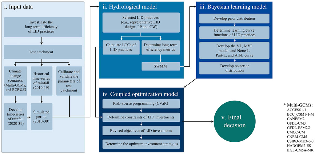
FIGURE 1. Flowchart of the methodology for the coupled Bayesian optimization model of LID investments. Note: PP, permeable pavement; CW, constructed wetland; LCC, life cycle cost; SWMM, Storm Water Management Model; VL, variance learning; MVL, mean-variance learning; None-L, none learning; Part-L, part learning; All-L, all learning; CVaR, conditional value at risk.

There are five main blocks in the work flow process: 1) preparation of input data and focusing on the hydrological characteristics of a test catchment; 2) select an appropriate hydrological model; the model is used for hydrologic simulation of stormwater runoff through the test catchments; 3) a Bayesian learning model which is used to assess the performance of LID practices under different investment strategies and various degrees of LID implementation; 4) a coupled optimization model which is used for developing the optimum investment strategy (optimum LID implementation); and 5) final decision module, in which the outcome of the above processes is used to determine the extent of the LID and its configuration such that the objective could be achieved optimally and with optimum investment.

Long-Term Efficiency of Low-Impact Development

Test Catchment and Climate Scenarios

Guangzhou, a high-density city in China, has the most severe urban flooding risk among the 136 large coastal cities in the world (Hallegatte et al., 2013). The rainfall distribution is non-uniform throughout the year due to the impacts of subtropical monsoon climate. Using selected multi-global climate models (GCMs) and the corresponding representative concentration pathways (RCPs) scenarios in Guangzhou, occurrences of extreme storms are expected to rise dramatically over the next 30 years (Zhang et al., 2017).

Two test catchments selected for this study were located at 23°04′ N; 113°12’ E, and they were residential sub-catchments S01 and S02 (Supplementary Figure S1). The land surface area of S01 and S02 included a different proportion of impermeable areas. The hydrologic parameters of both sub-catchments, as shown in Table 1, had been established and calibrated using ten rainfall events and validated using another 25 events over the period of 2013–15. The Kling–Gupta efficiency and Nash–Sutcliffe efficiency were above 0.7 and 0.6, respectively (Zhu et al., 2019).

TABLE 1

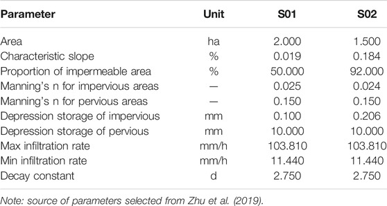
TABLE 1. Characteristic parameters of sub-catchment S01 and S02.

Historical rainfall data (2010–19) were collected from the rainfall station at the Baiyun International Airport, Guangzhou. In order to extract independent rainfall events from continuous time series, the inter-event time definition method with a duration of 12 h was adopted (Joo et al., 2014). “Future” rainfall data were established based on observed data and projections based on multi-GCMs (Figure 1) as well as RCPs introduced by IPCC in its Fifth Assessment Report (O'Neill et al., 2014). The median ensemble model of multi-GCMs was adopted to project rainfall events over the projected period. RCP 8.5, a high emission scenario reflecting the increasing greenhouse gas emissions leading to radiative forcing of 8.5 W/m² in 2,100, was selected as the climate change scenario (Lee et al., 2014). The projected period of 2020–39 was adopted. In so doing a 30-year planning horizon and LID’s life span (assumed to be 30 years) (Vineyard et al., 2015) was established, with the first 10 years (2010–19) of observed rainfall time series and 20 years (2020–39) of projected rainfall time series.

Hydrologic Model and LID Practices

The Storm Water Management Model (SWMM), a dynamic hydrologic model, was used to simulate the hydrological processes for a single and continuous rainfall event on an urban catchment. The result was used in the planning and design of various LID technologies (Kong et al., 2017). The underlying surface of catchment was treated as a non-linear reservoir (Palla and Gnecco, 2015). The Horton model for infiltration and dynamic wave routing was selected for rainfall loss and confluence routing (Rossman and Huber, 2016).

Although both PP and CW have been widely used in LID practices for reducing peak flow and pollution loads at source, their construction structures, materials, costs, and maintenance as well as applicabilities are quite different (Wang et al., 2019). In this study, PP and CW were adopted as representative LID elements, and the corresponding structural parameters are listed in Table 2. The surface area and width of the PP and CW were used to describe the extent of LID conceptually.

TABLE 2

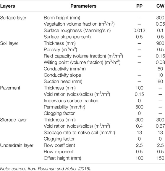
TABLE 2. Parameters of the permeable pavement (PP) and constructed wetland (CW) in SWMM.

Annual runoff volume reduction was set as the main parameter in the optimization (maximized cost-saving) of investment. The construction costs of LID practices are included in Table 3. The annualized maintenance costs were defined as a certain fraction of the capital costs, that is, 4.0% for PP and 8.0% for CW (Houle et al., 2013; Wang et al., 2020). The life cycle cost (LCC) of LID was a long-term cost over the service life time, and they were adopted as the investment budget. LCCs of PP and CW were calculated using the capital and maintenance costs over a service life time of 30 years (Rossman and Huber, 2016). Construction of PP and CWs was set to be ready at the beginning of year 1, while the maintenance costs were incurred at some point in time between years 1–30 (Wang et al., 2020). A present value (PV) accounting was performed by compiling all LCC and discounted to the 2018 United States dollar ($) value. The LCC of PP and CWs were calculated as:

$LCC=C_{\text{capital}}+P{V}_{O\&M},(1)$

$P{V}_{O\&M}={\displaystyle \sum }_{n=1}^{30}O\&M\frac{1}{{\left(1+i\right)}^n},(2)$

where $C_{\text{capital}}$ is the capital cost of LID, $P{V}_{O\&M}$ is the present value of the maintenance costs, $n$ is the number of year in service, and i is the discount rate reflecting the depreciation in value over time (Reis and Shortridge, 2020). A discount rate of 2% was adopted in this study (Dong, 2018).

TABLE 3

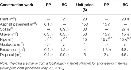
TABLE 3. Construction costs of constructed wetland (n m²) and permeable pavement (n m²) used in this study.

Long-Term Efficiency Metrics

Following the long-term performance modeling framework for LID developed by Liu et al. (2018), the effective performance of PP was assumed to degrade linearly over time and is shown in Figure 2A (Emerson et al., 2010; Haile et al., 2016). The decrease in PP effectiveness was mainly attributable to physical degradation such as clogging of the pores and sediment accumulation over the surface. Figure 2B shows the potential change in the mean CW effectiveness normally distributed during a typical year following the annual vegetative growth and decay cycle.

FIGURE 2

FIGURE 2. (A) Potential mean PP effectiveness during each year, (B) potential mean CW effectiveness during each year, and (C) example of composite mean PP and CW effectiveness over the design life span.

The composite efficiency of PP and CW is shown in Figure 2C. It is derived by superimposing the cyclic trend of the CW on the linearly decreasing trend of the PP. The relationship of $LS{E}_{mean\_PP}$ is as follow:

$LS{E}_{mean\_PP}=-a\times x+b,(3)$

where $a$ is the slope (assumed to have a default value of 0.020 ± 0.005) (Liu et al., 2018), and $b$ is the intercept set to 1, since the initial efficiency of PP was set to 100%.

The mean efficiency for CW ($LS{E}_{mean\_BC}$) was reflected as a series of normal distribution with attenuated magnitude (Figure 2C), which emulated the natural characteristics of decreasing efficiency from year-to-year. The ($LS{E}_{mean\_BC}$) was assumed normally distributed (Forbes et al., 2011) as:

$LS{E}_{mean\_BC}=pdf\_norm\left(x\mathrm{|}\sigma ,\mu \right)=\frac{1}{\sigma \sqrt{2\pi }}{e}^{\frac{-{\left(x-\mu \right)}^2}{2{\sigma }^2}},(4)$

where σ is the standard deviation (assumed to have a default value of 1.0 and a range of 0.5–5.0) (Liu et al., 2018); μ is the mean of x (assumed to be 0); and x has a value between −6 and +6 (the range of 12 months).

For the first year of CW’s service life, the highest mean efficiency ($LS{E}_{highest\_BC}$) was set to 100%. To reflect the downward trend of CW’s performance, $LS{E}_{highest\_BC}$ was assumed to decay with a reduction factor, $LS{E}_{nh}$ year-on-year:

$LS{E}_{highest\_BC}=100\mathrm{\%}\times {\left(1-LS{E}_{nh}\right)}^{N-1},(5)$

where N is the number of years of the design life span, and $LS{E}_{nh}$ reflects the progressive reduction of potential maximum efficiency year-on-year, and is assumed to have a default value of 2.0 ± 1.0%.

For the annual rainfall–runoff reduction, it was necessary to establish the statistics for the total runoff generated in the events for the y^th year as follow:

$R_{ov}\left(y\right)=V_y–{\displaystyle \sum }_{k=1}^{\text{n}}V\left(k,y\right)\times LS{E}_{mean},(6)$

where $R_{ov}\left(y\right)$ is the reduction runoff volume of LID practices in year y (from 2010–39), $V_y$ is the yth year annual runoff volume generated for non-LID catchment, n is the number of rain events in year y, and $LS{E}_{mean}$ is the mean efficiency of LID practices.

Bayesian Learning Programming

A Bayesian-based multi-stage decision model (with “prior” and “posterior” predictive distribution) was adopted to model the implementation process of the LID. The model analyzes various schemes of implementation, while considering opportunities and risks progressively. Certain schemes might change course at some future stages, depending on the level of achievement attained at that time. A two-stage decision model was incorporated in the LID scheme (investment decision) in this study. The main constraints were certain pseudo-random events and acceptable risk-averse levels.

“Prior” Distributions

According to the terminology of Bayesian inference theory, the distribution on the hydrological performances of LID practices at the initial stage, called the “prior” distribution, was assumed to be normally distributed ($\mu , {\sigma }^2$, where $\mu$ and ${\sigma }^2$ were the mean and variance of performances, respectively) based on the simulated ensemble of LID function units.

$P_{ave}\left(u,s\right)=\frac{1}{Y} \times \frac{{{\displaystyle \sum }}_{y=1}^Y{R}_{ov}\left(u,s\right)}{LCC\left(u,s\right)},\forall u\in \left\{\text{PP},\text{BC}\right\},\forall s\in \text{S},(7)$

where $P_{ave}\left(u,s\right)$ represents LID function objectives, $Y$ is 30 years of the simulated period, $u\in \left\{\text{PP},\text{BC}\right\}$ represented the investments in PP or CW, $s\in \text{S}$ represents the LID investment scenario s in S scenarios, and $R_{ov}\left(u,s\right)$ and $LCC\left(u,s\right)$ are the storm runoff volume reduction and life cycle costs for u LID type in scenario s, respectively. The LID function objective contains a single parameter, that is, storm runoff reduction. $P_{ave}\left(u,s\right)$ was therefore adopted as an index for average annual runoff volume reduction and reflected as reduced investment amount per $ per year in scenario s.

Learning Curve Function

A learning curve was assumed to be a function of the transformed relationship of investment on LID practices based on potential information gains from Bayesian Inference (Hung and Hobbs, 2019). These information gains were used to update the knowledge/beliefs regarding “posterior” distribution of the hydrological performance of LID practices in the second stage (Ferioli et al., 2009). A variance learning (VL) model and a mean-variance learning (MVL) model were proposed for various learning curve functions. The VL model was defined as a learning process which could only reduce the uncertainty of LID’s performance, whereas the MVL model assumed that the learning process could reduce uncertainty and improve the expected performance through technological advancement or cost reduction. Thus, the MVL model might be viewed as an extension of the VL model. The VL curve for variance reduction was expressed in the form of a two-step function (Figure 3A) representing one of the three possible learning pathways (None-L, Part-L, and All-L) that would take place. None-L was defined as one that the posterior distribution was identical to its prior; Part-L was defined as one that the posterior distribution variances were less than the prior distributions but not zero, and All-L was defined as one that the posterior distribution variance was set to zero. The learning curve function for reducing uncertainty of u LID solution in scenario s at Stage II (denoted Uncertainty ($x_{2\_s, u}$)) for both VL and MVL models was defined as follows.

$Uncertainty\left(x_{II,u,s}\right)=\beta {\sigma }^2\{\begin{array}{c}\beta =1,ifT{h}^{\text{Part}-\text{L}}>x_{II,u,s}\left(None-Ltakesplace\right)\\ 0<\beta <1,ifT{h}^{\text{Part}-\text{L}}\le x_{II,u,s}< T{h}^{\text{All}-\text{L}}\left(Part-Ltakesplace\right) \\ \beta =0,,ifT{h}^{\text{All}-\text{L}}\le x_{II,u,s}\left(All-Ltakesplace\right)\end{array},(8)$

where $\beta$ is a scaling constant that is used to adjust the variance. The parameters $T{h}^{\text{Part}-\text{L}}$ and $T{h}^{\text{All}-\text{L}}$ are the threshold values for investments needed for Part-L and All-L cases, respectively.

FIGURE 3

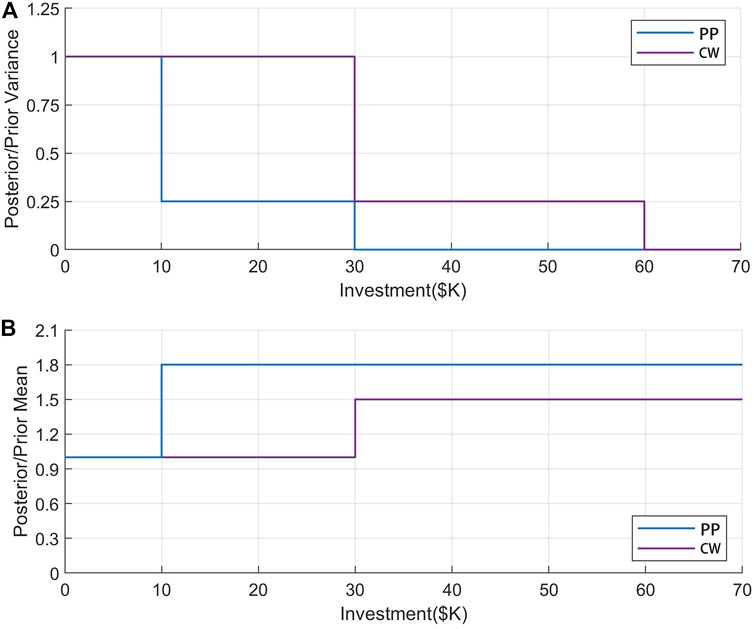
FIGURE 3. (A) Variance learning curve functions used in the VL and the MVL models and (B) learning curve functions for the expected value improvement in the MVL model.

In the MVL model, the learning curve function for mean improvement in scenario s of u LID type at Stage II (denoted by Mean ($x_{II, u, s}$)) is assumed to have a single level only, and has a threshold value equaled to $T{h}^{\text{Part}-\text{L}}$ (Figure 3B), as shown as below.

$\mathit{Mean}\left({\mathit{x}}_{II,u,s}\right)\{\begin{array}{c}\gamma \mu ,\gamma >1,ifT{h}^{\text{Part}-\text{L}}\le x_{II,u,s}\\ \mu ,if{x}_{II,u,s}<T{h}^{\text{Part}-\text{L}}\end{array},(9)$

where $\gamma$ is the scaling constant that could be used to adjust the posterior mean. The abscissa, investment ($), was indicated the extent/magnitude of LID.

Bayesian Optimization Formulation

The objective of the optimization process was to improve the relationship between LCC and the expected reductions in runoff volume based on the decision to invest on LID at various stages of development, and pending the resources, progressive learning, and risk constraints. Between expenditures and risk, tradeoffs were evaluated by adjusting the investment budget and risk appetite. Minimizing the risk of reduced efficiency was considered as one of the main considerations of investment on LID (Yamout et al., 2007). Conditional Value at Risk (CVaR), which reflects the average level of “portfolio excess loss,” is adopted as a reliable and valid index of the potential risk (Bakhtiari et al., 2019). This index was used as the index of “poor outcomes.” The optimization process portrayed risk-averse preferences by adopting CVaR constraints. If the constraint was binding, the decision was likely to be an investment that would elevate the expected performance under the worst risk conditions. The higher value of CVaR was desirable for maximum storm runoff volume reduction.

The VL model for investment optimization was calculated as follow:

$s_{opt}=arg\underset{s\in S}{\text{max}}\left[f{P}_{ave}\left(u,s\right)\right]=\text{Maximize }{f}_s\left(x_I,x_{II}\right),(10)$

$f_s\left(x_I,x_{II}\right)=\frac{1}{Y}\times \left\{C_{I,u,s}{x}_{I,u,s}+\frac{T_{II}}{T}\left[\frac{1}{S}{\displaystyle \sum }_{s=1}^S\left(C_{II\_n,u,s}{x}_{II\_n,u,s}+C_{II\_a,u,s}{x}_{II\_a, u, s}+C_{II\_p, u,s}{x}_{II\_p,u,s}\right)\right]\right\},(11)$

subject to

$\{\begin{array}{c}-x_{I,u}+T{H}_u^{\text{Part}}{L}_{Part,u}\le 0\\ -x_{I,u}+T{H}_u^{\text{All}}{L}_{All,u}\le 0\\ L_{None,u}+L_{Part,u}+L_{All,u}=1\end{array},\forall u\in \left\{\text{PP},\text{BC}\right\},(12)$

$\{\begin{array}{c}{z}_s\ge \tau -f_s\left(x_I,x_{II}\right),\forall s\in S\\ \tau -\frac{1}{\left(1-\alpha \right)S}{\displaystyle \sum }_{s=1}^S{z}_s\end{array},(13)$

where Eqs 12, 13 are learning and risk constraints, respectively; x is a decision variable; $x_I$, and $x_{II}$ are stage I, and II, respectively; $x_{II\_n,u,s}$, $x_{II\_p,u,s}$ and $x_{II\_a,u,s}$ are the investment vector at stage II for the None-L, Part-L, and All-L case in scenario s, respectively; $C_{I,u,s}$ is the reduction capacity of the storm runoff volume at stage I in scenario s; $C_{II\_n,u,s}$, $C_{II\_a,u,s}$, and $C_{II\_p,u,s}$ are the expected posterior mean of storm runoff volume reduction for the None-L, All-L, and Part-L cases at stage II in scenario s, respectively; $L_{None,u}$, $L_{Part,u}$ and $L_{All,u}$ are binary vector indicating whether (=1) or not (=0) None-L, Part-L, and All-L would occur for each of the $u$ LID types; $\tau$ is an auxiliary variable used to calculate CVaR; and $z_s$ is the stormwater reduction below $\tau$ in scenario s. In addition, it assumed equal likely of each scenario s.

The MVL model reflects technological improvement that would lead to added increase of the mean of the “posteriors” in comparison with the VL model. Therefore, the objective Eq. 10 may be revised as follow:

$\text{Maximize }{f}_s\left(x_I,x_{II}\right)=\frac{1}{Y}\times \left\{C_{I,u,s}{x}_{I,u,s}+\frac{T_{II}}{T}\left[\frac{1}{S}{\displaystyle \sum }_{s=1}^S\left(C_{II\_n,u,s}{x}_{II\_n,u,s}+C_{II\_a,u,s}^{MVL}{x}_{II\_a,u,s}+C_{II\_p,u,s}^{MVL}{x}_{II\_p,u,s}\right)\right]\right\},(14)$

where $C_{II\_a,u,s}^{MVL}$ and $C_{II\_p,u,s}^{MVL}$ are “posterior” mean of the storm runoff volume reduction rate for the All-L and Part-L cases in scenario s at stage II in the MVL model, respectively.

Discussion on the Assumptions Made

The constraints imposed on investment included the overall budget, learning relationships, and risk appetite. A budget per hectare of $100K was suggested for LID implemented at the test sub-catchment. Thus, the budgets for S01 and S02 were set to $200K and $150K, respectively. A two-stage investment process was developed to optimize the LID planning process. Stage I began at the start of the project, and Stage II would begin at year 4 in the 30-year planning horizon. Once installed, the LID would continue to generate storm runoff volume reduction until the end of the planning period.

The learning curves assumed in the VL model are displayed in Figure 3A. There, Uncertainty ($x_{II,u,s}$) = 1 indicated that the investment was below the threshold and would trigger learning; Uncertainty ($x_{II,u,s}$) = 0.25 meant that the investment would result in Part-L and the variance was reduced to a quarter of the original value. Here, Part-L thresholds corresponded to setting $10K and $30K for PP and CW, respectively. Uncertainty ($x_{II,u,s}$) = 0 meant that full information in All-L was obtained in Stage II so that the variance was reduced to zero. All-L thresholds corresponded to setting $30K and $60K for PP and CW, respectively. In the MVL model, the thresholds for 80 and 50% meant that improvements were assumed at setting $10K and $30K for PP and CW, respectively, and were the same as the Part-L thresholds in the VL model (Figure 3B). Besides, a lower bound value was placed on CVaR_0.05 as a minimal acceptable storm runoff volume reduction.

Results

“Prior” Distributions of the Performance of a Low-Impact Development

Statistically, the average annual rainfall from 2010 to 2019 was 2,253 mm. The climate ensemble of RCP 8.5 showed a small increase (0.9%) for the projected period (2020–39) of 2,272 mm for the median ensemble model. Although the median was close to that of the observed climate, the projected changes in monthly precipitation were still highly uncertain, especially in the monsoon. (Figure 4). The projected change in monthly precipitation in July ($\mu$ is 9.4 mm; ${\sigma }^2$ is 1,008.4 mm) is the most obvious, and its variance is nearly 110 times that in February. Figure 4 shows that Guangzhou could be subject to more severe urban flooding and drought due to significantly increased precipitation during the rainy season but decreasing rainfall during the dry season. Other studies focusing on climate change impacts reported similar findings (Huang et al., 2018). Deng et al. (2018) reported that seasonal storms and drought might occur more frequently with greater intensity in most areas of Guangzhou.

FIGURE 4

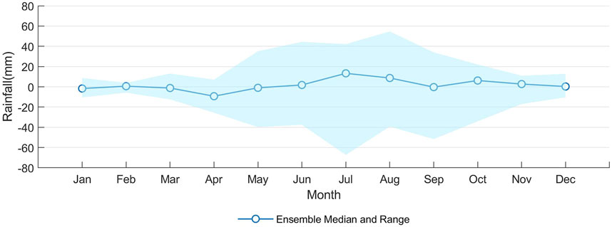
FIGURE 4. Projected changes in monthly precipitation compared to historical average data in Guangzhou during the simulated period for RCP 8.5. Note: source of information published by the Climate Change Knowledge Portal of the World Bank Group (https://climateknowledgeportal.worldbank.org [accessed 23 Jan 2020]).

Figure 5 illustrates the annualized storm runoff volume reduction, averaged over the 30-year time horizon. The performances of PP and CW showed a significant downward trend attributable to decreasing efficiency based on the long-term performance curves of LIDs. It was noted that the performance curves were calculated according to the average performance as recorded in the long-term time series for both LIDs. Therefore, extreme scenarios would not be reflected within the scenario of a particularly stable long-term performance or rapid degradation. At the end of service life, long-term effectiveness of PP would remain between 25.0 and 55.0% and appeared normally distributed. However, in its last year of service life, the highest efficiencies of CW would range from 10.0 to 70.0% with greater fluctuation.

FIGURE 5

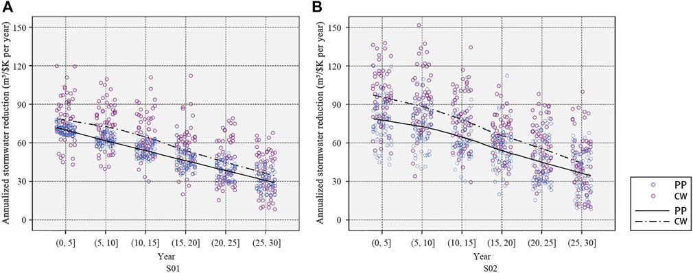
FIGURE 5. Annualized stormwater reduction of LIDs in (A) S01 and (B) S02 based on the long-term effectiveness analysis in a simulated period.

More frequent heavy rainfall events following climate change would have exceeded the LID’s drainage capacity and reduce the hydrological efficiency of LID. The performance of CW was found to be superior than that of PP in S01 and S02 during the same period. Also, the efficiency of storm runoff volume reduction through LID in S01 was relatively lower than that in S02. This result was attributed to the lower impervious rate in S01, which led to lower rainfall losses and hence lower runoff volume reduction.

By calculating the “prior” distribution of LIDs based on long-term effectiveness, the performances of both LIDs appeared normally distributed. CVaR_0.05 was used to calculate the risk values of “prior” probability for LIDs under long-term performance (Figure 6). As a result, investment on CW was found to be more cost-efficient than that for PP, but the uncertainty with the performance of CW was higher. Also, CW showed lower CVaR values, reflecting its potentially higher risk. These findings were found to be consistent with those reported by others (Liu et al., 2018). It was noted that the unit performance of LID in S02 was better than that in S01 but it also showed a significant level of uncertainty.

FIGURE 6

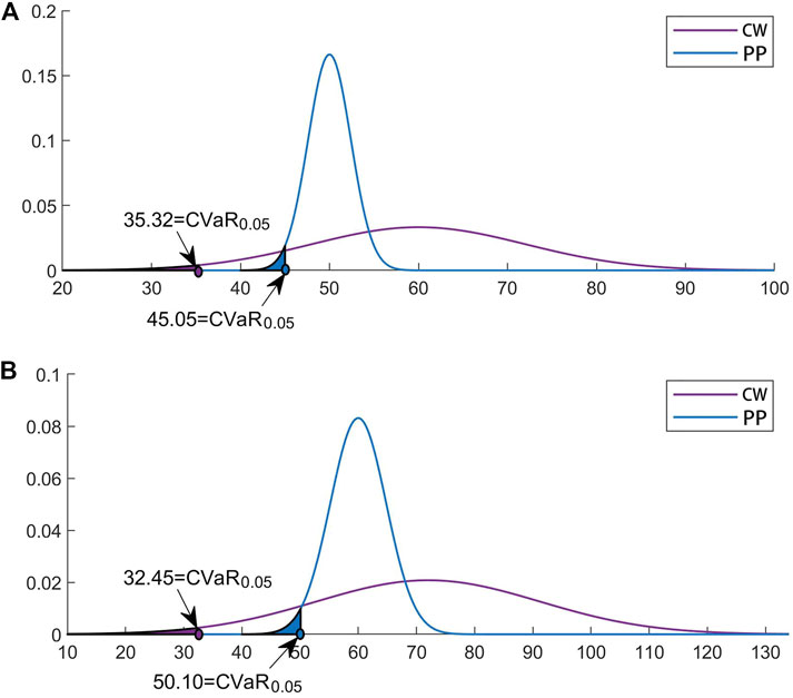
FIGURE 6. Prior distribution of LIDs with normal distribution in (A) S01 and (B) S02.

Variance Learning Model

Though the same unit budget (a budget of $100K per hectare {assumed}) was invested in LID, the performance and risk thresholds corresponding to different test catchments were different (Figure 7). The VL model was examined for CVaR_0.05 with values ranging from 7,060 m³/yr to 9,678 m³/yr in S01 and 4,815 m³/yr to 7,980 m³/yr in S02. S01, at a CVaR of 7,060 m³/yr, which was the alternative that maximizes the expected storm runoff volume reduction, achieved a value of 12,000 m/yr. High value of CVaR had higher stability at the expense of lower expected hydrological performance. CVaR could increase to as much as 9,678 m³/yr, with an increase of 37.1%. However, the corresponding expected storm runoff volume reduction was reduced by about 7.0% from 12,000 to 11,160 m³/yr. Thus, it appeared that the risk capacity determined the expected reduction of runoff. Meanwhile, CVaR showed a 65.7% increase from 4,815 m³/yr to 7,980 m³/yr, while the expected storm runoff volume reduction fell about 23.3% from 10,800 m³/yr to 8,280 m³/yr in S02.

FIGURE 7

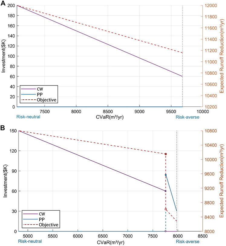
FIGURE 7. Investment strategies at Stage I (left axis) and the objective function values (right axis) from the VL model for CVaR0.05 in (A) S01 and (B) S02.

Not surprisingly, the optimal strategy was one in which all allotted budgets were invested in CW at Stage I for a risk-neutral decision-maker since CW had proven track of good performance with a higher “prior” mean, even if PP were to degrade more slowly than CW, and CW only portrayed a marginally higher effectiveness than PP at around the middle of each year from Figure 2. It is worth noting that the average annual runoff control over the service life time was adopted as the performance level in this study. Limited hydrological management ability of CW in the later period was ignored, since CW degrades faster than PP over time.

There was no strong incentive to invest in PP or take advantage of learning on the VL model since “to wait” means that there would be no derived benefit during the initial 3 years, which then led to lower surface runoff reduction over the 30-year period. However, were him showed a risk-averse attitude, the manager might act to save some amount of budget for the next stage or mix his investment with more LID alternatives, or to wait to obtain better estimates of LID performance. For instance, when 7,060 m³/yr < CVaR ≤ 9,678 m³/yr, the model suggested making investments in CW and also saving some amount of budget for Stage II.

In the case of S02, the optimal solutions were more complex. With 4,815 m³/yr < CVaR ≤ 7,758 m³/yr, the model suggested making investments in CW, while saving some amount of budget to leverage on “All-L” in CW. However, with 7,758 m³/yr < CVaR ≤ 7,980 m³/yr, the model suggested investing in PP to the tune of $85.5K to $30K for “All-L″ at Stage I and saving the balance to invest at Stage II in order to further reduce the risk. It was noted that CVaR showed a 2.9% increase from investing in CW to PP. However, the expected storm runoff volume reduction decreased dramatically by about 18.4% from 10,152 to 8,280 m³/yr. Note that PP was not recommended for the risk-neutral decision-makers since its efficacy is limited, but it was added for the conservative or risk-averse one due to its obvious stability of hydrological performance.

Mean-Variance Learning Model

The MVL model added other sets of learning functions to the VL model, for which the expected performances of PP and CW could be improved. As a result, the MVL model depicted a lower incentive to make investment at Stage I to increase the expected volume reduction, as compared to the VL model. A recommended initial decision is to make a partial or delayed investment first, and then decide when more information becomes available. The losses at Stage I may increase, but better long-term outcomes could be achieved by reducing the loss of structural performance and potential technological change for LID, since it avoids irreversible investment at the initial stage and retains the option of future expansion (Gersonius et al., 2013). Meanwhile, the expectation is one with the highest return when the investment strategy is extremely risk averse. This means that aggressive and high-risk investment strategies at the initial stage do not necessarily lead to high expectations when considering the uncertainty of technological development.

Figure 8 illustrates the expected storm runoff volume reduction as a function of CVaR_0.05. The objective values in MVL models were higher than the results in VL models due to anticipated technological improvements with a decrease in capital costs or an increase in hydrological efficiency for a “new” LID device. Moreover, with an increased CVaR value, the expected runoff volume reduction showed an upward trend of fluctuation, which was the opposite of the VL model. For instance, in S01, CVaR could be significantly increased from 7,060 m³/yr to 15,415 m³/yr, and the corresponding expected storm runoff volume reduction increased by about 32.4%, from 12,000 to 15,890 m³/yr. This was the result of investing a limited amount of budget at Stage I to activate technological improvements, resulting in the reductions of posterior variance and an expected increase in LID. With the assumed technological improvement, the CVaR value could be as high as 15,415 m³/yr and 13,490 m³/yr in S01 and S02, respectively. In the VL model, the CVaR had a cup of 10,000 m³/yr in both sub-catchments, whereas the maximum expected storm runoff volume reduction in the MVL model increased by about 32.4 and 40.0% for S01 and S02, respectively, when compared with the VL model. It was also noted that, in S01, and with CVaR set to 13,480 m³/yr or higher, the MVL also suggested investment of more than $10K in PP in Stage I to obtain “Part-L” for improving the efficiency of LID. Here, PP was not invested in the VL model as PP had a higher potential to enhance its performance with a relatively lower uncertainty in Stage II.

FIGURE 8

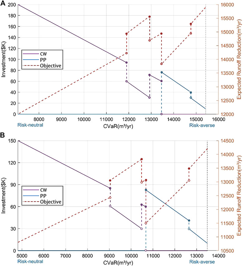
FIGURE 8. Investment strategies at Stage I (left axis), and the objective function values (right axis) from the MVL model for CVaR0.05 in (A) S01 and (B) S02.

Conclusion

A coupled long-term efficiency analysis of LID and a Bayesian learning model has been proposed. The model has the ability to minimize urban flooding risk and maximize expected storm runoff volume reduction through optimal investment in LID. As a dynamic decision-making tool, the model could be implemented in stages with deliberate decision to invest more or suspend investment on the LID elements at various times, pending the observed performance (progressive updates of performance) of the LID, resources available, environmental changes, technological advancement, and users’ needs and expectations. Each and every stage of the development is to be designed and built after a Bayesian update of the probabilistic performance function for each LID option. The goal of this Bayesian update is to support the engineers and administrators on the improvement of the design and investment, respectively, by having to minimize uncertainty and to maximize returns leveraging on potential technological advancements and reducing cost. The proposed framework and procedure can also be applied to the planning and investment planning in other fields that involve some degree of uncertainty. Despite the successful illustration of the framework reported herein, the authors emphasize that simulation of long-term LID efficiencies and the modification/validation of learning curves based on the Bayesian method can be further enhanced. A rapid and efficient method for calibration and verification for the data-driven Bayesian model needs to be further investigated.

Data Availability Statement

The raw data supporting the conclusions of this article will be made available by the authors, without undue reservation.

Author Contributions

MW: conceptualization, methodology, writing—original draft preparation, and supervision; YuZ: software, data curation, and visualization; DZ: methodology, validation, and supervision; YiZ: formal analysis, investigation, and data curation; SZ: software, data curation, and visualization; ST: methodology, validation, and supervision.

Funding

This work was supported by the National Natural Science Foundation of China (grant number 51808137) and the Natural Science Foundation of Guangdong Province (grant number 2019A1515010873).

Conflict of Interest

The authors declare that the research was conducted in the absence of any commercial or financial relationships that could be construed as a potential conflict of interest.

Publisher’s Note

All claims expressed in this article are solely those of the authors and do not necessarily represent those of their affiliated organizations, or those of the publisher, the editors, and the reviewers. Any product that may be evaluated in this article, or claim that may be made by its manufacturer, is not guaranteed or endorsed by the publisher.

Supplementary Material

The Supplementary Material for this article can be found online at: https://www.frontiersin.org/articles/10.3389/fenvs.2021.713831/full#supplementary-material

References

Ahiablame, L. M., Engel, B. A., and Chaubey, I. (2012). Effectiveness of Low Impact Development Practices: Literature Review and Suggestions for Future Research. Water Air Soil Pollut. 223 (7), 4253–4273. doi:10.1007/s11270-012-1189-2

CrossRef Full Text | Google Scholar

Ahiablame, L., and Shakya, R. (2016). Modeling Flood Reduction Effects of Low Impact Development at a Watershed Scale. J. Environ. Manage. 171, 81–91. doi:10.1016/j.jenvman.2016.01.036

CrossRef Full Text | Google Scholar

Bahrami, M., Bozorg-Haddad, O., and Loáiciga, H. A. (2019). Optimizing Stormwater Low-Impact Development Strategies in an Urban Watershed Considering Sensitivity and Uncertainty. Environ. Monit. Assess. 191 (6), 340. doi:10.1007/s10661-019-7488-y

PubMed Abstract | CrossRef Full Text | Google Scholar

Bakhshipour, A. E., Dittmer, U., Haghighi, A., and Nowak, W. (2019). Hybrid green-blue-gray Decentralized Urban Drainage Systems Design, a Simulation-Optimization Framework. J. Environ. Manage. 249, 109364. doi:10.1016/j.jenvman.2019.109364

CrossRef Full Text | Google Scholar

Bakhtiari, P. H., Nikoo, M. R., Izady, A., and Talebbeydokhti, N. (2019). A Coupled Agent-Based Risk-Based Optimization Model for Integrated Urban Water Management. Sustain. Cities Soc. 53, 101922. doi:10.1016/j.scs.2019.101922

CrossRef Full Text | Google Scholar

Bracmort, K. S., Arabi, M., Frankenberger, J., Engel, B. A., and Arnold, J. G. (2006). Modeling long-term water quality impact of structural BMPs. T. ASABE. 49 (2), 367–374. doi:10.13031/2013.20411

CrossRef Full Text | Google Scholar

Chen, H., Grieneisen, M. L., and Zhang, M. (2016). Predicting Pesticide Removal Efficacy of Vegetated Filter Strips: A Meta-Regression Analysis. Sci. Total Environ. 548-549, 122–130. doi:10.1016/j.scitotenv.2016.01.041

PubMed Abstract | CrossRef Full Text | Google Scholar

Deng, S., Chen, T., Yang, N., Qu, L., Li, M., and Chen, D. (2018). Spatial and Temporal Distribution of Rainfall and Drought Characteristics across the Pearl River basin. Sci. Total Environ. 619-620, 28–41. doi:10.1016/j.scitotenv.2017.10.339

PubMed Abstract | CrossRef Full Text | Google Scholar

Dong, Y. (2018). Performance Assessment and Design of Ultra-high Performance concrete (UHPC) Structures Incorporating Life-Cycle Cost and Environmental Impacts. Construction Building Mater. 167, 414–425. doi:10.1016/j.conbuildmat.2018.02.037

CrossRef Full Text | Google Scholar

Emerson, C. H., Wadzuk, B. M., and Traver, R. G. (2010). Hydraulic Evolution and Total Suspended Solids Capture of an Infiltration Trench. Hydrol. Process. 24 (8), 1008–1014. doi:10.1002/hyp.7539

CrossRef Full Text | Google Scholar

Ferioli, F., Schoots, K., and van der Zwaan, B. C. C. (2009). Use and Limitations of Learning Curves for Energy Technology Policy: A Component-Learning Hypothesis. Energy Policy 37 (7), 2525–2535. doi:10.1016/j.enpol.2008.10.043

CrossRef Full Text | Google Scholar

Forbes, C., Evans, M., Hastings, N., and Peacock, B. (2011). Statistical Distributions. John Wiley & Sons.

Google Scholar

Gersonius, B., Ashley, R., Pathirana, A., and Zevenbergen, C. (2013). Climate Change Uncertainty: Building Flexibility into Water and Flood Risk Infrastructure. Climatic Change 116 (2), 411–423. doi:10.1007/s10584-012-0494-5

CrossRef Full Text | Google Scholar

Haile, T. M., Hobiger, G., Kammerer, G., Allabashi, R., Schaerfinger, B., and Fuerhacker, M. (2016). Hydraulic Performance and Pollutant Concentration Profile in a Stormwater Runoff Filtration Systems. Water Air Soil Pollut. 227 (1), 34. doi:10.1007/s11270-015-2736-4

CrossRef Full Text | Google Scholar

Hallegatte, S., Green, C., Nicholls, R. J., and Corfee-Morlot, J. (2013). Future Flood Losses in Major Coastal Cities. Nat. Clim Change 3 (9), 802–806. doi:10.1038/nclimate1979

CrossRef Full Text | Google Scholar

Hou, J., Han, H., Qi, W., Guo, K., Li, Z., and Hinkelmann, R. (2019). Experimental Investigation for Impacts of Rain Storms and Terrain Slopes on Low Impact Development Effect in an Idealized Urban Catchment. J. Hydrol. 579, 124176. doi:10.1016/j.jhydrol.2019.124176

CrossRef Full Text | Google Scholar

Houle, J. J., Roseen, R. M., Ballestero, T. P., Puls, T. A., and Sherrard, J. (2013). Comparison of Maintenance Cost, Labor Demands, and System Performance for LID and Conventional Stormwater Management. J. Environ. Eng. 139 (7), 932–938. doi:10.1061/(asce)ee.1943-7870.0000698

CrossRef Full Text | Google Scholar

Huang, H., Chen, X., Zhu, Z., Xie, Y., Liu, L., Wang, X., et al. (2018). The Changing Pattern of Urban Flooding in Guangzhou, China. Sci. Total Environ. 622-623, 394–401. doi:10.1016/j.scitotenv.2017.11.358

PubMed Abstract | CrossRef Full Text | Google Scholar

Hung, F., and Hobbs, B. F. (2019). How Can Learning-By-Doing Improve Decisions in Stormwater Management? A Bayesian-Based Optimization Model for Planning Urban green Infrastructure Investments. Environ. Model. Softw. 113, 59–72. doi:10.1016/j.envsoft.2018.12.005

CrossRef Full Text | Google Scholar

Jacobi, S. K., Hobbs, B. F., and Wilcock, P. R. (2013). Bayesian Optimization Framework for Cost-Effective Control and Research of non-point-source Sediment. J. Water Resour. Plann. Manage. 139 (5), 534–543. doi:10.1061/(asce)wr.1943-5452.0000282

CrossRef Full Text | Google Scholar

Joo, J., Lee, J., Kim, J. H., Jun, H., and Jo, D. (2014). Inter-event Time Definition Setting Procedure for Urban Drainage Systems. Water 6 (1), 45–58. doi:10.3390/w6010045

CrossRef Full Text | Google Scholar

Kelly, D. L., and Kolstad, C. D. (1999). Bayesian Learning, Growth, and Pollution. J. Econ. Dyn. Control. 23 (4), 491–518. doi:10.1016/s0165-1889(98)00034-7

CrossRef Full Text | Google Scholar

Koch, B. J., Febria, C. M., Gevrey, M., Wainger, L. A., and Palmer, M. A. (2014). Nitrogen Removal by Stormwater Management Structures: A Data Synthesis. J. Am. Water Resour. Assoc. 50 (6), 1594–1607. doi:10.1111/jawr.12223

CrossRef Full Text | Google Scholar

Kong, F., Ban, Y., Yin, H., James, P., and Dronova, I. (2017). Modeling Stormwater Management at the City District Level in Response to Changes in Land Use and Low Impact Development. Environ. Model. Softw. 95, 132–142. doi:10.1016/j.envsoft.2017.06.021

CrossRef Full Text | Google Scholar

Larsen, T. A., Hoffmann, S., Lüthi, C., Truffer, B., and Maurer, M. (2016). Emerging Solutions to the Water Challenges of an Urbanizing World. Science 352 (6288), 928–933. doi:10.1126/science.aad8641

PubMed Abstract | CrossRef Full Text | Google Scholar

Lee, J. W., Hong, S. Y., Chang, E. C., Suh, M. S., and Kang, H. S. (2014). Assessment of Future Climate Change over East Asia Due to the RCP Scenarios Downscaled by GRIMs-RMP. Clim. Dynam. 42 (3-4), 733–747. doi:10.1007/s00382-013-1841-6

CrossRef Full Text | Google Scholar

Liu, R., Chen, Y., Wu, J., Gao, L., Barrett, D., Xu, T., et al. (2017). Integrating Entropy-Based Naïve Bayes and GIS for Spatial Evaluation of Flood Hazard. Risk Anal. 37 (4), 756–773. doi:10.1111/risa.12698

PubMed Abstract | CrossRef Full Text | Google Scholar

Liu, Y., Ahiablame, L. M., Bralts, V. F., and Engel, B. A. (2015). Enhancing a Rainfall-Runoff Model to Assess the Impacts of BMPs and LID Practices on Storm Runoff. J. Environ. Manage. 147, 12–23. doi:10.1016/j.jenvman.2014.09.005

CrossRef Full Text | Google Scholar

Liu, Y., Engel, B. A., Flanagan, D. C., Gitau, M. W., McMillan, S. K., Chaubey, I., et al. (2018). Modeling Framework for Representing Long-Term Effectiveness of Best Management Practices in Addressing Hydrology and Water Quality Problems: Framework Development and Demonstration Using a Bayesian Method. J. Hydrol. 560, 530–545. doi:10.1016/j.jhydrol.2018.03.053

CrossRef Full Text | Google Scholar

Montalto, F., Behr, C., Alfredo, K., Wolf, M., Arye, M., and Walsh, M. (2007). Rapid Assessment of the Cost-Effectiveness of Low Impact Development for CSO Control. Landscape Urban Plann. 82 (3), 117–131. doi:10.1016/j.landurbplan.2007.02.004

CrossRef Full Text | Google Scholar

O’Neill, B. C., Kriegler, E., Riahi, K., Ebi, K. L., Hallegatte, S., Carter, T. R., et al. (2014). A New Scenario Framework for Climate Change Research: the Concept of Shared Socioeconomic Pathways. Climatic Change 122 (3), 387–400.

CrossRef Full Text | Google Scholar

Palla, A., and Gnecco, I. (2015). Hydrologic Modeling of Low Impact Development Systems at the Urban Catchment Scale. J. Hydrol. 528, 361–368. doi:10.1016/j.jhydrol.2015.06.050

CrossRef Full Text | Google Scholar

Pyke, C., Warren, M. P., Johnson, T., LaGro, J., Scharfenberg, J., Groth, P., et al. (2011). Assessment of Low Impact Development for Managing Stormwater with Changing Precipitation Due to Climate Change. Landscape Urban Plann. 103 (2), 166–173. doi:10.1016/j.landurbplan.2011.07.006

CrossRef Full Text | Google Scholar

Reis, J., and Shortridge, J. (2020). Impact of Uncertainty Parameter Distribution on Robust Decision Making Outcomes for Climate Change Adaptation under Deep Uncertainty. Risk Anal. 40, 494–511. doi:10.1111/risa.13405

PubMed Abstract | CrossRef Full Text | Google Scholar

Rossman, L. A., and Huber, W. (2016). Storm Water Management Model Reference Manual Volume I–Hydrology. Cincinnati, OH, USA: US Environmental Protection Agency.

Google Scholar

Shi, R., Hobbs, B. F., and Jiang, H. (2019). When Can Decision Analysis Improve Climate Adaptation Planning? Two Procedures to Match Analysis Approaches with Adaptation Problems. Climatic Change 157, 611–630. doi:10.1007/s10584-019-02579-3

CrossRef Full Text | Google Scholar

Sturm, M., Goldstein, M. A., Huntington, H., and Douglas, T. A. (2017). Using an Option Pricing Approach to Evaluate Strategic Decisions in a Rapidly Changing Climate: Black–Scholes and Climate Change. Clim. Chang. 140 (3-4), 437–449. doi:10.1007/s10584-016-1860-5

CrossRef Full Text | Google Scholar

Tang, X., Shu, Y., Lian, Y., Zhao, Y., and Fu, Y. (2018). A Spatial Assessment of Urban Waterlogging Risk Based on a Weighted Naïve Bayes Classifier. Sci. Total Environ. 630, 264–274. doi:10.1016/j.scitotenv.2018.02.172

PubMed Abstract | CrossRef Full Text | Google Scholar

Thompson, J., Sattar, A. M. A., Gharabaghi, B., and Warner, R. C. (2016). Event-based Total Suspended Sediment Particle Size Distribution Model. J. Hydrol. 536, 236–246. doi:10.1016/j.jhydrol.2016.02.056

CrossRef Full Text | Google Scholar

Vineyard, D., Ingwersen, W. W., Hawkins, T. R., Xue, X., Demeke, B., and Shuster, W. (2015). Comparing green and Grey Infrastructure Using Life Cycle Cost and Environmental Impact: a Rain Garden Case Study in Cincinnati, OH. J. Am. Water Resour. Assoc. 51 (5), 1342–1360. doi:10.1111/1752-1688.12320

CrossRef Full Text | Google Scholar

Wang, M., Zhang, D., Cheng, Y., and Tan, S. K. (2019). Assessing Performance of Porous Pavements and Bioretention Cells for Stormwater Management in Response to Probable Climatic Changes. J. Environ. Manage. 243, 157–167. doi:10.1016/j.jenvman.2019.05.012

CrossRef Full Text | Google Scholar

Wang, M., Zhang, D., Wang, Z., Zhou, S., and Tan, S. K. (2021). Long-term Performance of Bioretention Systems in Storm Runoff Management under Climate Change and Life-Cycle Condition. Sustain. Cities Soc., 102598. doi:10.1016/j.scs.2020.102598

CrossRef Full Text | Google Scholar

Wang, Z., Zhou, S., Wang, M., and Zhang, D. (2020). Cost-benefit Analysis of Low-Impact Development at Hectare Scale for Urban Stormwater Source Control in Response to Anticipated Climatic Change. J. Environ. Manage. 264, 110483. doi:10.1016/j.jenvman.2020.110483

CrossRef Full Text | Google Scholar

Webster, M., Fisher-Vanden, K., Popp, D., and Santen, N. (2017). Should We Give up after Solyndra? Optimal Technology R&D Portfolios under Uncertainty. J. Assoc. Environ. Resource Economists 4 (S1), S123–S151. doi:10.1086/691995

CrossRef Full Text | Google Scholar

Woodward, M., Kapelan, Z., and Gouldby, B. (2014). Adaptive Flood Risk Management under Climate Change Uncertainty Using Real Options and Optimization. Risk Anal. 34 (1), 75–92. doi:10.1111/risa.12088

PubMed Abstract | CrossRef Full Text | Google Scholar

Yamout, G. M., Hatfield, K., and Romeijn, H. E. (2007). Comparison of New Conditional Value-At-Risk-Based Management Models for Optimal Allocation of Uncertain Water Supplies. Water Resour. Res. 43 (7). doi:10.1029/2006wr005210

CrossRef Full Text | Google Scholar

Yazdanfar, Z., and Sharma, A. (2015). Urban Drainage System Planning and Design - Challenges with Climate Change and Urbanization: a Review. Water Sci. Technol. 72 (2), 165–179. doi:10.2166/wst.2015.207

PubMed Abstract | CrossRef Full Text | Google Scholar

Yuan, Z., Liang, C., and Li, D. (2018). Urban Stormwater Management Based on an Analysis of Climate Change: A Case Study of the Hebei and Guangdong Provinces. Landscape Urban Plann. 177, 217–226. doi:10.1016/j.landurbplan.2018.04.003

CrossRef Full Text | Google Scholar

Zhang, H., Wu, C., Chen, W., and Huang, G. (2017). Assessing the Impact of Climate Change on the Waterlogging Risk in Coastal Cities: A Case Study of Guangzhou, South China. J. Hydrometeorol. 18 (6), 1549–1562. doi:10.1175/jhm-d-16-0157.1

CrossRef Full Text | Google Scholar

Zhu, Z., Chen, Z., Chen, X., and Yu, G. (2019). An Assessment of the Hydrologic Effectiveness of Low Impact Development (LID) Practices for Managing Runoff with Different Objectives. J. Environ. Manage. 231, 504–514. doi:10.1016/j.jenvman.2018.10.046

CrossRef Full Text | Google Scholar