CrowdQC+—A Quality-Control for Crowdsourced Air-Temperature Observations Enabling World-Wide Urban Climate Applications

Introduction

Cities modify atmospheric conditions and amongst these alterations the urban heat island (UHI) phenomenon, i.e., generally higher temperatures within the city compared to its rural surroundings, is likely the best documented one (Arnfield 2003; Oke et al., 2017; Stewart 2019). Despite high variability in atmospheric conditions within cities due to heterogeneity in underlying surface cover, morphology, thermal properties, and anthropogenic heat emissions (Oke et al., 2017), there is a dearth of observations to monitor these. While a growing number of cities is now equipped with dedicated urban climate observation networks (see review by Muller et al., 2013), mostly run by research institutions [e.g., Amsterdam, Netherlands (Ronda et al., 2017), Berlin, Germany (Fenner et al., 2014; Langer et al., 2021), Birmingham, United Kingdom (Chapman et al., 2015; Warren et al., 2016), Novi Sad, Serbia (Šećerov et al., 2019), Szeged, Hungary (Lelovics et al., 2014; Skarbit et al., 2017)], for the broad majority of urban regions across the globe little to none is known about their urban climate conditions through observations.

In recent years, the collection and utilisation of vast amounts of data via crowdsourcing, i.e., the collection of data from non-traditional sources via the internet (Muller et al., 2015), has gained much attention. Such non-traditional, opportunistic sources of data are, e.g., smartphones (e.g., Overeem et al., 2013b; Mass and Madaus 2014; Droste et al., 2017), smart wearable devices (Nazarian et al., 2021), cars (e.g., Haberlandt and Sester 2010; Bartos et al., 2019), commercial microwave links (e.g., Messer et al., 2006; Overeem et al., 2013a; Chwala and Kunstmann 2019), and privately-owned weather stations, called citizen weather stations (CWS) in the following (e.g., Steeneveld et al., 2011; Wolters and Brandsma 2012; Bell et al., 2013; Madaus et al., 2014; Chapman et al., 2017; de Vos et al., 2017; Venter et al., 2021). Each type of these data sources alone or multiple combined can be used in different meteorological and climatological applications, such as weather forecast (e.g., Mass and Madaus, 2014; Nipen et al., 2020), operational weather monitoring (e.g., de Vos et al., 2019), mesoscale model evaluation (e.g., Hammerberg et al., 2018), hydrometeorological analyses and modelling (e.g., Smiatek et al., 2017; de Vos et al., 2020), high-resolution mapping of air temperature (e.g., Venter et al., 2020; Vulova et al., 2020; Zumwald et al., 2021), thermal-comfort assessment (Nazarian et al., 2021), and urban climate investigations (e.g., Fenner et al., 2017, 2019; Droste et al., 2020; Feichtinger et al., 2020). The potential of CWS data is especially large for cities, where population density and thus also CWS network density is high and where traditional meteorological observations are sparse.

By investigating CWS data and crowdsourced data sets of air-temperature (ta) measurements, Bell et al. (2015) and Meier et al. (2017) identified different sources of uncertainties or errors. These are issues related to metadata (e.g., incorrect, incomplete), the device design (flaws of the station that lead to inaccurate measurements, e.g., radiative errors, slow response), installation (e.g., CWS set up inappropriately near building walls), calibration (e.g., constant offsets or sensor drift over time), and communication and software errors (lead to missing data) (Bell et al., 2015; Meier et al., 2017). For other variables than ta, other sources of uncertainty may also arise [see, e.g., de Vos et al. (2019) for precipitation, and Droste et al. (2020) for wind speed]. Design flaws leading to radiative errors and to slow sensor-response times are common among many different types of CWS (Bell 2015). This holds particularly true for the Netatmo CWS (https://www.netatmo.com/en-us/weather), a popular CWS especially in Europe. Due to its compact built form and its aluminium shell with poor ventilation and without a proper radiation screen it is particularly affected by both types of errors (Meier et al., 2017; Büchau 2018). Despite the abundance of CWS, especially in urban areas, crowdsourced CWS data sets can hence not be used in urban climate research without prior rigorous quality control (QC).

To address sources of uncertainties associated with CWS data and to remove erroneous data from a data set of crowdsourced CWS observations, a number of studies has developed QC procedures, either relying on reference data from professionally-operated weather stations (PRWS), or using statistical approaches that are independent of additional meteorological observations. Several QC procedures for CWS that make use of PRWS data have been developed, all with different complexity and focusing on different variables: for ta (e.g., Bell 2015; Meier et al., 2017; Hammerberg et al., 2018; Cornes et al., 2020), for precipitation (Bárdossy et al., 2021), for wind speed (Droste et al., 2020; Chen et al., 2021), and for multiple variables (Clark et al., 2018; Mandement and Caumont 2020). Recently, Båserud et al. (2020) introduced an automatic QC package for ta and precipitation, which aims at identifying possibly faulty values from meteorological observations based on a series of (spatial) tests. The applicability of that specific QC is highlighted by the fact that it is implemented in the operational weather forecast of the Norwegian Meteorological Service (Båserud et al., 2020; Nipen et al., 2020).

One core potential benefit of CWS data is their availability in regions where traditional and high-quality meteorological observations are sparse or even non-existing. Hence, a QC that is independent of such additional data makes it particularly useful for application in such areas and transferable across regions. For precipitation from CWS, de Vos et al. (2019) developed an automatic QC that can be applied in (near-)real time for operational weather monitoring. For ta, Chapman et al. (2017), e.g., used a relatively simple statistical approach of mean and standard deviation to filter potentially faulty measurements from CWS in London, United Kingdom. Napoly et al. (2018) developed a more comprehensive QC for ta, also working without reference meteorological data and being available as a package in R (R Core Team 2021) under the name of “CrowdQC” (Grassmann et al., 2018). CrowdQC is a statistically-based QC with four main and three optional QC levels that are applied sequentially, removing erroneous data based on the assumption that the whole crowd of CWS knows more than each individual station (“wisdom of the crowd”). Since its release, CrowdQC has successfully been applied in a number of studies to quality-control CWS ta data for further analyses (e.g., Fenner et al., 2019; Feichtinger et al., 2020; Venter et al., 2020, 2021; Vulova et al., 2020; Benjamin et al., 2021; Potgieter et al., 2021; Zumwald et al., 2021). Its large-scale applicability was only recently demonstrated by the study of Venter et al. (2021), using CrowdQC to quality-control data from >50,000 CWS in 342 urban regions in Europe for a summer month.

While CrowdQC already provides good performance regarding identifying and removing possibly faulty values in the CWS data set (Napoly et al., 2018), Feichtinger et al. (2020), e.g., identified that when applying CrowdQC for Vienna, Austria, radiative errors remained in the filtered data set. Similar issues were reported by Venter et al. (2021). To address the remaining radiative errors, Feichtinger et al. (2020) introduced additional filter levels, adopting filter functions developed by Meier et al. (2017). These additional filter functions rely on measurements of global radiation and ta data from PRWS. Further, Feichtinger et al. (2020) had to collect and quality-control a whole month of CWS data, even though their investigation period lasted only eleven days during that month. This was due to the functionality of CrowdQC, which only worked on a fixed monthly basis and not being flexible towards periods of other lengths.

While radiative errors have been addressed by the various QC procedures available for CWS data, none of them has tried to address errors due to slow sensor response. Sensor-response times are dependent on the type of sensor, its built form, radiation shield, location, and weather conditions, which makes it non-trivial to implement such a correction for crowdsourced CWS data. The question is, whether it is nonetheless possible to reduce such errors due to slow sensor response, in absence of additional meta data and other meteorological observations. Since Netatmo CWS are all built identically, it might be possible to reduce errors in a crowdsourced data set of hundreds of these CWS in a simplified manner by correcting the data with a uniform time constant.

This study introduces and describes CrowdQC+ as a further development of CrowdQC. CrowdQC+ builds on its predecessor, keeping the QC concepts, software and QC design, and existing QC levels. The core aim of CrowdQC+ is to retain the existing applicability of CrowdQC, i.e., providing a QC for CWS data that is independent of reference meteorological data, thus exploiting the “wisdom of the crowd” and being applicable universally around the world. The main idea of CrowdQC+ is that there is trustworthy information in a large group of individual measurements, which can be used to check individual values. With several enhancements and added functionalities, the aim of CrowdQC+ is to increase applicability and performance of the QC, effectively removing faulty data while retaining as much data as possible. The core enhancement of CrowdQC+ is the introduction of two new QC levels: The first implements a spatial QC that mainly addresses radiative errors, the second a temporal correction of the data regarding sensor-response time. Besides, a number of modifications and bug fixes to the existing package are implemented, as well as several helper functions that target the user-friendliness of the package.

The following sections aim at providing on overview of the open-source package CrowdQC+ with its additional functionalities and extensions. Both CrowdQC and CrowdQC+ are applied to two data sets in Amsterdam (Netherlands) and Toulouse (France), where PRWS data exist, used as benchmark. In the end, two applications highlight the applicability of CWS data in urban climate research.

Data and Methods

Data

Cities and Investigation Periods

Two cities were selected for this study: Amsterdam (52.37°N, 4.89°E) and Toulouse (43.60°N, 1.44°E). Figure 1 displays both regions and corresponding weather stations, Table 1 provides a brief overview of the cities and the respective investigation periods. Both investigation periods cover 1 year: 2019 and 2020 for Amsterdam and Toulouse, respectively. The cities and investigation periods were selected due to the availability of reference data from PRWS for comparison with CWS data, relatively dense CWS networks, different background climates, and different city settings.

FIGURE 1

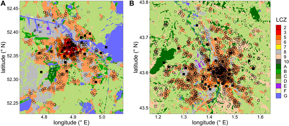
FIGURE 1. Study regions (A) Amsterdam and (B) Toulouse with the location of weather stations and Local Climate Zones LCZ. Citizen weather stations (raw data availability) are displayed as black circles, professionally-operated weather stations as black squares. A more detailed description of the LCZ scheme can be found in Stewart & Oke (2012).

TABLE 1

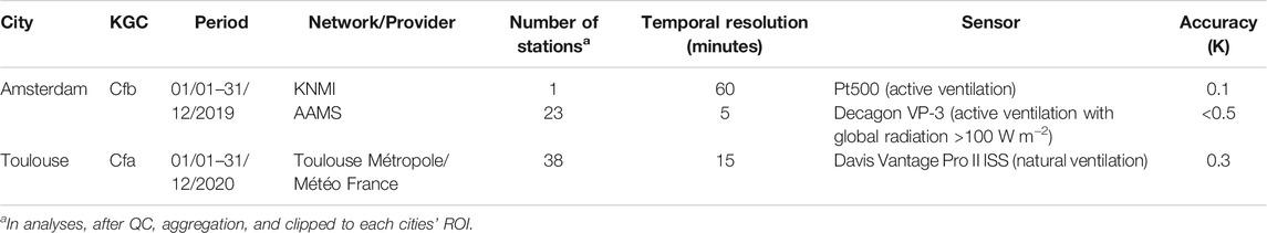
TABLE 1. Overview of the professionally-operated weather stations in each city used in the investigations. KGC: Köppen-Geiger classification after Beck et al. (2018b). KNMI, Koninklijk Nederlands Meteorologisch Instituut–Royal Netherlands Meteorological Institute; AAMS, Amsterdam Atmospheric Meteorological Supersite (Ronda et al., 2017).

Amsterdam lies in the north of the Netherlands and is strongly influenced by maritime air from the North Sea (distance to coast <50 km). In addition, the surroundings contain large waterbodies (to the north-east of the city) and canals are found throughout the city centre region. The region of interest (ROI) for Amsterdam (cf. definition of ROI in Station Selection section) has a flat topography, with an altitude approximately at mean sea level. Central areas of the city are mainly composed of LCZ 2 (compact midrise). Surrounding these areas, LCZ 6 (open low-rise) and 8 (large low-rise) dominate the built-up areas, natural surroundings of the city are mainly composed of LCZ D (low plants) and G (water) (Figure 1A).

Toulouse is an inland city in the south of France, approximately 80 km north/north-east of the Pyrenees mountain range. The river Garonne runs through the city. Overall, topography is flat, with a mean ROI altitude of approximately 150 m above mean sea level (amsl). Central parts of Toulouse are composed of LCZ 2 and 5 (open midrise), while largest built-up areas consist of LCZ 6, 8, and 9 (sparsely built). Natural landcover surrounding the city is mainly LCZ D and A (dense trees) (Figure 1B).

Citizen Weather Stations and Crowdsourcing

Data from CWS were collected from the Netatmo network (https://weathermap.netatmo.com/) via the company’s Application Programming Interface API (https://dev.netatmo.com/).

The Netatmo CWS is a smart device, sold by the French company “Netatmo.” The station consists of an indoor and an outdoor module, each enclosed by a cylindrical shell made of aluminium. Upon purchase, Netatmo CWS do not contain a proper radiation shield such as lamella-type radiation screens, making it prone to shortwave radiative errors if set up in unshaded locations. Additional radiation screens can be fitted to the sensor but are likely only found at a marginal percentage of Netatmo CWS, since the company does not offer such a screen. The outdoor module measures ta (specified accuracy ±0.3 K, −40°C to 65°C) and relative humidity at 5-min resolution. Data is automatically and wirelessly sent to the Netatmo server, from which the owner can retrieve the data. If the owner consents to share the data, the outdoor measurements are publicly shared and can be retrieved via the API at no cost. Meier et al. (2017) investigated the accuracy of the sensor, showing that the specified accuracy is met for the tested range 0°C–30°C, with only a small positive bias at 0°C. Fenner (2020) further showed that even after several years in the field the sensors did not show a systematic drift and still met the specified accuracy.

CWS ta data was crowdsourced at an hourly resolution using the “getmeasure” API endpoint. Beforehand, station metadata (station identifier, latitude, longitude, altitude) were collected and updated regularly using the “getpublicdata” API endpoint, retrieving new metadata and comparing it to previously-obtained metadata. Each CWS received a unique internal station ID. If a change in position for an existing CWS was detected, a new internal station ID was assigned to this CWS, in order to keep the time series consistent (similar to Meier et al., 2017). Metadata for each CWS are limited to geographical position and altitude, and no further information regarding, e.g., a possible additional radiation shield or the specific setup of the sensor are available from the Netatmo API. This is in contrast to other CWS platforms such as Weather Underground (https://www.wunderground.com/pws/overview) or the Weather Observations Website (https://www.wow.metoffice.gov.uk/), where such metadata can be provided by station owners and which can then be obtained by API users. However, the Netatmo network surpasses other CWS platforms regarding network density, especially in Europe, and offers the advantage of a consistent station design and sensor quality throughout the whole network.

Netatmo CWS data are one-hourly mean values. Netatmo time stamps obtained from the API were valid for the beginning of each aggregation interval, which was modified (+3600 s/+1 h) to represent the end of each interval. Then, CWS data were prepared for the QC according to the requirements of the CrowdQC and CrowdQC+ packages, resulting in a data table (Dowle and Srinivasan 2021) with column names as required by the packages [ta, time information, station ID, and corresponding coordinates (latitude, longitude)].

Professionally-Operated Weather Stations and Quality Control

Data from PRWS were collected from different institutions for both cities. The respective temporal availability, temporal resolution, instrumentation, and number of stations are displayed in Table 1. Data from these PRWS are especially suitable for our purpose, as networks in both cities cover extended areas with stations being located in a variety of local settings, yet with a focus on city-centre regions where CWS data are also especially dense (Figure 1). PRWS data for Amsterdam from the Amsterdam Atmospheric Meteorological Supersite (AAMS, Ronda et al., 2017) have previously been used in the evaluation of and comparison with CWS data (e.g., de Vos et al., 2020; Droste et al., 2020). PRWS data from the network in Toulouse was already used in the study by Napoly et al. (2018) to evaluate the performance of CrowdQC, yet with a much lower number of sites than in this study. Sensors of both PRWS networks are installed on lampposts or street signs at a height of approximately 3–4 m above ground level.

Data from PRWS were quality-controlled to remove unrealistic values. The QC steps and corresponding thresholds were adapted from several sources (Shafer et al., 2000; Zahumenský 2004; Fiebrich et al., 2010; Estévez et al., 2011; Cerlini et al., 2020). The QC consisted of four individual tests, all working on the individual station level:

1) Gross-error limit test: All values outside the range [−40°C, 60°C] were flagged as FALSE.

2) Spike-dip/step test (temporal consistency): If the difference between a value and its previous value was above a threshold value, this value was flagged as FALSE. The threshold was adapted to the temporal resolution of the data (5-min resolution: 6 K, 15-min resolution: 10 K, 1-hourly resolution: 20 K).

3) Persistence test (temporal consistency): If a value persisted for a certain period of time, these values were flagged as FALSE. The threshold was adapted to the temporal resolution of the data (5-min resolution: 2 h, 15-min resolution: 3 h, 1-hourly resolution: 6 h).

4) Manual visual check: This last step was performed to identify any additional flawed data based on a visual inspection of each time series.

The QC tests were always applied at the highest available temporal resolution at each station. If any of the tests failed (FALSE flag), this value was set to missing value. After QC, all data were aggregated to hourly mean values. A minimum of >80% of valid data per hour had to be available for the aggregation, otherwise this value was set to missing value. Further, each month of a station was only kept if >80% of hourly data were valid.

Local Climate Zone Maps

For each city, an LCZ map (Figure 1) was produced using the LCZ Generator (Demuzere et al., 2021, https://lcz-generator.rub.de/). This web application translates the default WUDAPT protocol (Bechtel et al., 2015; Ching et al., 2018) into a cloud-based web application, thereby using all recent advancements of LCZ mapping as described in Bechtel et al. (2019) and Demuzere et al. (2019a,b; 2020).

Methods

Station Selection

A ROI was set for each city. Each ROI extended from the minimum to the maximum in common geographical coverage among the PRWS and CWS networks (based on latitude and longitudes of all stations), adding (subtracting) 0.05° to the maximum (minimum) latitude and longitude. Only stations within each ROI were selected for further analyses (Figure 1). The ROI for Amsterdam (506.54 km²) is about half the size of that for Toulouse (1,130.90 km²), while the maximum network density in time for raw CWS data (calculated per hourly data availability) is similar for both cities with 0.85 CWS/km² and 0.86 CWS/km² for Amsterdam and Toulouse, respectively.

Height Correction

For comparisons among stations after QC, ta data were corrected for elevation differences among stations to a reference height per city, using the environmental lapse rate of −0.0065 K m⁻¹. The reference height was set to the mean of the elevation of all PRWS in each city, rounded to the nearest integer value (Amsterdam: 3 m amsl, Toulouse: 155 m amsl). The elevation of each station was extracted from the nearest grid-point value from the hole-filled Shuttle Radar Topographic Mission SRTM data (Jarvis et al., 2008). Additionally, the sensor height was considered in the height correction, using the available metadata for PRWS and assuming a uniform sensor height for the CWS of 2 m above ground level, as in Fenner et al. (2017).

Classification of Stations to Local Climate Zones

All CWS available in the ROI were considered in the application of CrowdQC and CrowdQC+. For comparison between CWS and PRWS, an LCZ was assigned to each station following Fenner et al. (2017) and Varentsov et al. (2021), using the geographical position of each station and the LCZ maps. First, the nearest-pixel LCZ value was assigned to each station. Second, for a buffer with a radius of 250 m around each station, the surface-cover fraction of the modal LCZ was calculated (using pixels of the LCZ map). Third, a weighted surface-cover LCZ fraction in the same buffer was calculated (Varentsov et al., 2021), applying “similarity weights” (Figure 3B in Bechtel et al., 2020) between the modal LCZ and all other grid points (LCZ pixels) within the buffer.

Only those stations (CWS and PRWS) were considered if 1) the nearest-pixel LCZ was identical to the modal LCZ in the buffer, 2) the modal LCZ covered a surface fraction within the buffer of >0.5, and 3) the weighed-LCZ fraction of the modal LCZ was ≥0.75. This procedure was applied to select only those stations that are located in homogeneous surroundings regarding the LCZ scheme, to obtain a locally-representative signal (Fenner et al., 2017).

Statistics

Four statistical metrics were calculated to compare CWS with PRWS ta data.

Mean deviation MD:

$MD= \frac{1}{N}{\displaystyle \sum _{i=1}^{N}t{a}_{i, CWS}-t{a}_{i,PRWS}}$

where ta_i,CWS and ta_i,PRWS are ta at CWS and PRWS, respectively, at time i.

Mean absolute deviation MAD:

$MAD= \frac{1}{N}{\displaystyle \sum _{i=1}^N\left|t{a}_{i, CWS}-t{a}_{i,PRWS}\right|}$

Root-mean-square deviation RMSD:

$RMSD= \sqrt{\frac{1}{N}{\displaystyle \sum }_{i=1}^N{(t{a}_{i, CWS}-t{a}_{i,PRWS})}^2}$

Centred root-mean-square deviation cRMSD (Taylor 2001):

$cRMSD= \sqrt{\frac{1}{N}{\displaystyle \sum _{i=1}^N{\left[\left(t{a}_{i, CWS}-\overline{t{a}_{i,CWS}}\right)-\left(t{a}_{i,PRWS}-\overline{t{a}_{PRWS}}\right)\right]}^2}}$

where $\overline{t{a}_{CWS}}$and $\overline{t{a}_{PRWS}}$are temporal mean ta across the whole investigation period at CWS and PRWS, respectively.

For comparisons when these statistical metrics were calculated per PRWS (e.g., Table 3), all CWS within a 2000 m radius around each PRWS, belonging to the same LCZ as the PRWS (cf. Classification of Stations to Local Climate Zones section), where firstly identified (Amsterdam: 200 CWS from 531 in the original data retained, Toulouse: 497 CWS from originally 1,354). Secondly, the metrics were calculated for each of these CWS-PRWS pairs and then averaged per PRWS. Lastly, the metrics where averaged across all PRWS for city-scale results. This approach was chosen in order to have an as direct as possible comparison between the two types of networks, even though a large percentage of CWS was omitted. If the statistical metrics were calculated on the network basis, i.e., averaging ta per network first and then calculating the metrics, overall lower deviations were obtained (not shown).

Description of CrowdQC+

CrowdQC+ is an improved version of the existing CrowdQC R package (Grassmann et al., 2018; Napoly et al., 2018), implementing several additional or modified functionalities. In the following, all available functions are briefly described. Focus is given to the additions and modifications of CrowdQC+. Table 2 provides an overview of the QC levels and additional functions that are available.

TABLE 2

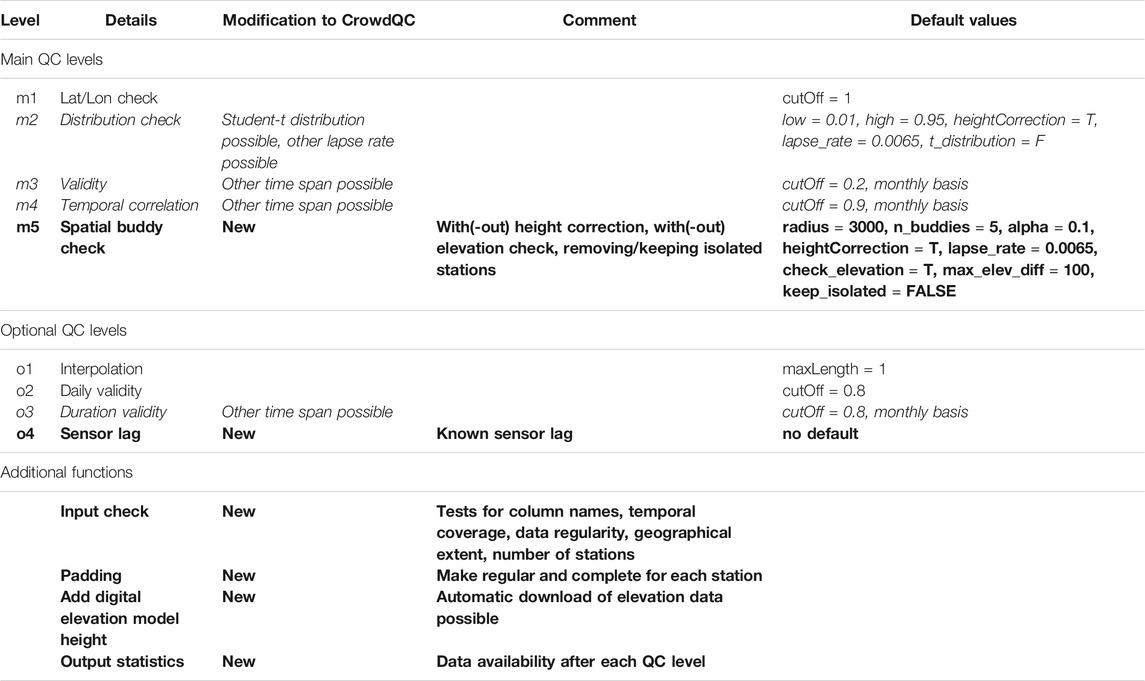
TABLE 2. Overview of the quality control QC levels and additional functions available in CrowdQC+. Italic lines mark functions that were modified regarding their functionality compared to the original CrowdQC, bold lines mark functions that were added in CrowdQC+.

As in CrowdQC, a data table with CWS data and meta data is used as input in CrowdQC+. Each QC level adds an additional column to the data table with boolean flag values TRUE (QC level passed) and FALSE (QC level failed). Only values flagged TRUE in the previous QC level are used in the subsequent level.

Main Quality-Control Levels

m1–Metadata Check

In QC level m1, function cqcp_m1 performs a metadata check based on available latitude and longitude values and removes stations with identical values (similar also to filter A0 in Meier et al., 2017). This function is unchanged compared to CrowdQC and primarily targets CWS that were faultily installed by the user with automatic assignment of geographic coordinates based on the IP address of the user’s internet connection. This error is a common feature in data sets of Netatmo CWS.

m2–Distribution Check

In main QC level m2 the distribution of ta at each time step for the whole ROI is checked and values that are statistical outliers at the lower and upper ends of the distribution are removed. Respective cut-off values can be specified by the user. This QC level primarily targets radiative errors that lead to unrealistically high ta values, and errors due to CWS installed indoors, showing, e.g., lower ta during daytime than CWS installed outdoors. A height correction, i.e., lapse-rate adjustment of ta, can be applied (default: TRUE) to account for elevation differences in the data set. Compared to CrowdQC, where only the environmental lapse rate could be applied, cqcp_m2 now provides the option to the user to specify any lapse rate in the height correction. Then, a normal distribution is assumed in QC level m2 to calculate critical values for flagging outliers at the lower and upper ends of the distribution at each time step. Yet, if the available number of stations is low (<100, value discussed in Effect of Different Distribution Functions in m2 section), the assumption of normal distribution may no longer hold. In such a case, critical values can be more robustly calculated assuming a Student-t distribution (Gosset, 1908). This functionality (parameter “t_distribution”) was added in CrowdQC+.

m3–Data Validity

Main QC level m3 checks each station for the amount of values that were flagged FALSE in QC level m2. If too many values (default: 20%) are flagged FALSE in a certain period of time, it is assumed that this station is to erroneous to be kept. In CrowdQC this period of time was fixed to monthly episodes. In CrowdQC+, cqcp_m3 offers the possibility to specify any period of time (“duration”) for this check. The user can also choose to use the complete data set (“complete = TRUE”).

m4–Temporal Correlation

In QC level m4, a temporal correlation between each station and the median of all stations is carried out for a specified period of time. As in QC level m3, this was formerly set to correlations per month. In cqcp_m4, analogously to cqcp_m3, any period of time can be specified or the complete data set can be used (default: month). If the complete data set or the specified duration is short (sample size <100) considering the temporal resolution of the data set, the correlation is still calculated, yet a warning is given. This QC level primarily targets CWS that are set up indoors and thus show a weak temporal correlation with the median of all CWS, which are assumed to be installed outdoors.

m5–Spatial Buddy Check

This new main QC level m5 performs a spatial buddy check, i.e., an outlier detection within the neighbourhood of a station. Analogously to QC level m2, it is assumed that a (large) number of individual observations contain robust information, justifying that individual stations can be flagged as erroneous when deviating too much from spatially adjacent stations. This QC level aims at identifying faulty values that remained after all previous QC steps, primarily single unrealistically high values due to radiative errors. The QC level is comparable to the spatial buddy check implemented in the TITAN package (Båserud et al., 2020). There, mean and standard deviation are calculated across the buddies to then identify statistical outliers. For CrowdQC+, it was decided to apply the same robust statistics in the buddy check as in QC level m2, i.e., median and Q_n estimator (Rousseeuw and Croux, 1993), the latter being an efficient alternative of the median absolute deviation, instead of the arithmetic mean and standard deviation. CWS data sets typically contain outliers that could affect these statistics, while median and Q_n/median absolute deviation are less influenced by them.

In cqcp_m5, the spatial neighbours, i.e., buddies, of each station are first identified within a given radius (default: 3000 m). If a sufficiently large number of neighbours with valid data are available (default: five), median and Q_n are calculated per time step, excluding the station that is checked. Then, comparable to the check in cqcp_m2 (see Napoly et al., 2018 for the detailed description), a z-score Z is calculated as

$Z=\left|\frac{t{a}_{i,j}-median\left(t{a}_{i, buddies}\right) }{Q_n\left(t{a}_{i, buddies}\right)}\right|$

where ta_i,j is the ta value at time i and station j, and ta_i,buddies are the ta values of the buddies at time i. Based on the Student-t distribution and a specified significance level a (default: 0.1), critical cut-off values (two-tailed approach, default: a = 0.1, which translates to probabilities of 0.05 and 0.95 at the lower and upper tail of the distribution, respectively) are calculated per station and time step. All values for which Z < cut-off and for which the number of buddies is sufficiently high are flagged as TRUE, otherwise FALSE. Additionally, a second column “isolated” is added to the data table, indicating whether (flag “isolated” = FALSE) or not (flag “isolated” = TRUE) enough buddies are present for each station.

In order to avoid the influence of vertical temperature gradients in this check, the data can be corrected for height differences using a lapse-rate adjustment, as in cqcp_m2 (default: TRUE). This is done prior to the statistical calculations detailed above. Additionally, and independently from the height correction, the user can specify that only stations within the radius are considered, if their elevation does do differ too much from the elevation of the station that is checked (default: 100 m elevation difference).

Since at least the specified number of buddies/valid observations has to be present within the given radius, QC level m5 also flags isolated stations (flag “m5” = FALSE). While this will lead to the exclusion of stations and negatively affect spatial coverage, it provides greater trust in the overall quality-controlled data set, since data from individual CWS are doubtful in absence of comprehensive metadata (Fenner et al., 2017; Napoly et al., 2018). Nonetheless, for certain applications or especially where network density is low, it might be desirable to keep these isolated stations, which an optional parameter allows (“keep_isolated = TRUE”).

By setting the minimum number of buddies to a low number or specifying a large radius, the user has the possibility to adjust this to the region under investigation, depending on, e.g., network density.

Optional Quality-Control Levels

After the main QC levels, four optional levels are included in CrowdQC+. Altogether, they aim at further improving data quality, yet are not considered essential. The benefits of these levels depend on the specific application.

o1–Temporal Interpolation

In optional QC level o1, function cqcp_o1 carries out a temporal linear interpolation for missing values between the two closest valid values in a time series. This function is unchanged compared to CrowdQC and aims at increasing data availability by having as continuous time series as possible.

o2–Daily Validity

For robust calculation of daily values, function cqcp_o2 checks if a predefined fraction (default: 0.8) of valid values is available at each station on each calendar day. Again, this QC level is unchanged compared to CrowdQC.

o3–Validity in Time Period

Optional QC level o3 was modified compared to CrowdQC to handle other time spans than full months, to be consistent with the main QC levels m3 and m4. Function cqcp_o3 checks if a predefined fraction (default: 0.8) of valid values is available at each station during the specified duration.

o4–Correction for Time Constant

The optional QC level o4 was introduced in CrowdQC+ in order to correct values for a known time constant τ of the sensor at each station. τ is typically defined as the time that a sensor needs to respond to approximately 63% of a step change in conditions (here: ta). Typical high-quality sensors deployed in meteorological measurement networks have τ values of a few seconds. However, CWS might suffer from design flaws, leading to a slow response time of the sensor (Bell et al., 2015). Netatmo sensors, e.g., have a slow thermal response due to their compact form and cylindrical enclosure, as noted by previous works (Meier et al., 2017; Büchau 2018).

In function cqcp_o4, a time-constant corrected air temperature ta_corr is calculated (similar to Miloshevich et al., 2004 for humidity):

$ta\_cor{r}_i=\frac{t{a}_i-\left(t{a}_{i-1}\ast e^{-\raisebox{1ex}{$\left(t_i-t_{i-1}\right)$}\!\left/ \!\raisebox{-1ex}{$\tau $}\right.}\right)}{1-e^{-\raisebox{1ex}{$\left(t_i-t_{i-1}\right)$}\!\left/ \!\raisebox{-1ex}{$\tau $}\right.}}$

where ta_i is the ta value at time t_i, ta_i-1 the ta value at the previous time step t_i-1, e Euler’s number, and τ the time constant.

In CrowdQC+ it is assumed that τ is the same for all stations and that it is constant, regardless of weather conditions. In the correction itself, it is assumed that a step change in air temperature happens from one time step to the next. The correction is applied to the original values (“ta”) and not to the interpolated values obtained in QC level o1 (“ta_int”). Hence, the correction can be applied after any QC level. Diverging from all other QC levels, no additional flag variable with TRUE/FALSE values is added to the data table during cqcp_o4. The user can thus select the corrected values at any QC level. In addition, cqcp_o4 is not carried out with any default values, as the time constant is specific to each possible sensor type. CrowdQC+ is, however, not limited or specific to any type of station or sensor.

Additional Functions

On top of the actual QC functions, four additional functions are implemented in CrowdQC+ to provide the user with support in preparing the input data for the QC and to obtain quick statistics on data availability at each QC level. These functions do not carry out actual QC of the data.

Input Check

The cqcp_check_input function checks the input data table for compliance with CrowdQC+ and can be used before starting the actual QC functions. Five individual tests are performed to check that 1) all relevant columns (“p_id”, “time”, “ta”, “lon”, “lat”) are present, 2) the temporal coverage of all stations is identical, 3) data for all stations are at the same temporal resolution and regular, 4) the geographical extent is not too large (<100 km×100 km), and 5) the absolute number of available stations is sufficiently high. The function prints information regarding these tests in the console or to an output file, or outputs the results of the tests as a list. The latter output is especially useful in automated workflows. The function further provides hints to the user to resolve errors in case some of the tests fail.

Padding

The padding function cqcp_padding makes sure that all stations cover the same period of time with the same temporal resolution and is helpful in the preparation of the data for CrowdQC+. For a specified temporal resolution, data at each station is set to the nearest, next upper, or previous lower time step. If multiple values per time step are present, the mean is calculated across these. This function is especially useful if, e.g., the original station data have gaps, do not cover the same period of time, or have time stamps that are not regular.

Adding Digital Elevation Model Height

If the user does not have elevation information at each station available but wants to apply the height correction of the measurement data in main QC levels m2 and m5, cqcp_add_dem_height adds data from a digital elevation model (DEM) to each station. Any DEM data can be provided by the user via a RasterLayer object or a path to a GeoTIFF. If none of the two is given, SRTM data is downloaded automatically via the getData function from the raster package (Hijmans 2021). The downloaded data can be cropped to the extent of the CWS data and stored as a GeoTIFF. Note that SRTM data is only available between 60°N and 56°S. In case the region under investigation is located outside that range the user should make use of other available DEM data sets, e.g., the “Multi-Error-Removed Improved-Terrain DEM (MERIT DEM)” (Yamazaki et al., 2017).

Output Statistics

After CrowdQC+ was carried out, cqcp_output_statistics provides basic statistics, i.e., the absolute number of valid observations, the percentage of valid observations compared to the raw data, and the number of unique stations with at least one valid observation after each QC level. The information is printed to the console or to an output file. This function is for illustrative purposes to the user to see, e.g., what effect the choice of a different threshold in one of the QC functions has on data availability.

Results and Analyses of New Functionalities

In this section, mainly the results for Amsterdam are shown as figures and tables. Similar figures and tables for Toulouse can be found in Supplementary Material A and will be referred to in the following sub-sections.

Overall Performance and Comparison With CrowdQC

Comparing overall deviations between CWS and PRWS in Amsterdam, both QC packages show a strong improvement in all statistical metrics along the annual cycle compared to the raw data, except for MD (Figure 2). MD is higher after applying the QC packages compared to the raw data. This is due to the fact that a large number of CWS in Amsterdam show values just above 0°C and around −20°C (Figure 3A) at the raw data level. These stations are likely set up indoors in refrigerated warehouses or fridges, as they also display no distinct annual cycle but display relatively constant values. Similar features were noticed by Meier et al. (2017) for likely indoor stations in Berlin, which showed relatively constant values around 20°C. After applying the QC functions, both data sets are cleaned of these outliers by misplaced CWS (Figure 3B, Supplementary Figure S2).

FIGURE 2

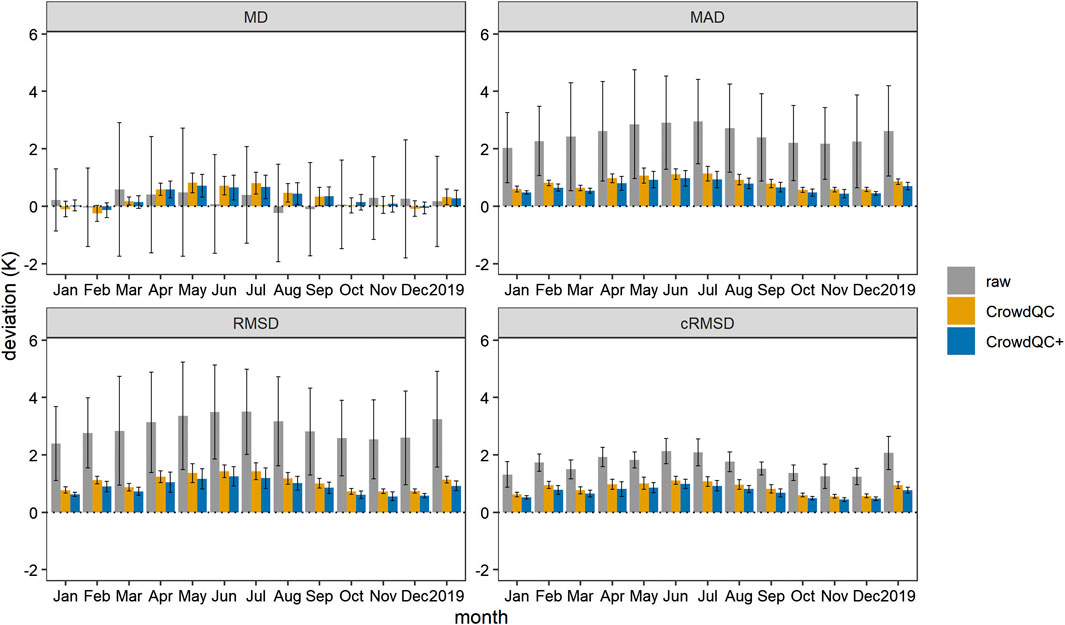
FIGURE 2. Deviations in hourly air temperature (ta) between CWS and PRWS in Amsterdam during 2019 per month and for the whole year. Displayed are values for the raw data set, after applying CrowdQC and CrowdQC+ in their respective default settings (cf. Table 2). Shown are values at QC level o3. Deviations were calculated between each PRWS and each CWS within a radius of 2000 m around the respective PRWS, located in the same LCZ type as the PRWS. Deviations were then averaged per month and year across all CWS and PRWS. Error bars denote the standard deviation across all CWS and PRWS per month and year. MD, mean deviation; MAD, mean absolute deviation; RMSD, root-mean-square deviation; cRMSD, centred RMSD.

FIGURE 3

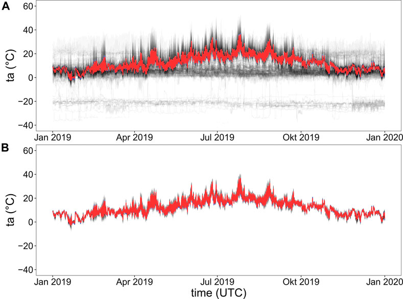
FIGURE 3. Hourly air temperature (ta) in Amsterdam during 2019. Each grey line corresponds to data from a single CWS, the red line displays the spatial median across all CWS, the blue line the median across all PRWS (barely visible as similar to red line). Sub-figure (A) shows raw CWS data, sub-figure (B) CWS data at QC level m5 of CrowdQC+ with default settings (cf. Table 2).

Overall, positive deviations are visible in CWS ta compared to PRWS ta (Figure 2, Supplementary Figure S1), as noted in previous studies (e.g., Chapman et al., 2017; Meier et al., 2017; Napoly et al., 2018; Venter et al., 2021). Deviations are reduced after application of CrowdQC and CrowdQC+, with stronger reduction for Amsterdam than for Toulouse. Statistical metrics further show that while CrowdQC already provides a strong improvement compared to the raw data, CrowdQC+ provides further improvement with overall lower deviations than CrowdQC (Figure 2, Supplementary Figure S1). Improvements are stronger during the warmer months of the year for all metrics in Amsterdam and more variable for Toulouse (Supplementary Figure S1). Comparing both cities, Amsterdam shows generally lower deviations than Toulouse and displays a more distinct annual cycle with higher deviations during summer compared to winter months (Figure 2).

The overall better performance of CrowdQC+ is, however, accompanied with lower data availability after QC (Table 3). QC level m1 already reduced data availability by 30% and removed 163 CWS for Amsterdam. The high percentage of invalid values at QC level m1 is specific to the Amsterdam CWS data set and much higher than for Toulouse (Table 3) and what was found for Berlin, Germany (Meier et al., 2017; Napoly et al., 2018). In fact, most of these removed CWS in Amsterdam with invalid latitude and longitude values as defined by QC level m1 show no distinct annual cycle in ta (not shown) and are thus likely set up indoors. QC filters m2 and m5 (CrowdQC+) further reduced data availability by approximately 10% in both cities. Due to the reduction in data availability in QC level m5, roughly 20% of the raw CWS data at nearly 200 CWS are retained after QC level o3 with CrowdQC+ in Amsterdam, compared to 41% from 281 CWS with CrowdQC (Table 3). For Toulouse, the difference in data availability after QC level o3 between CrowdQC and CrowdQC+ is similar, with approximately 55% and nearly 30%, respectively.

TABLE 3

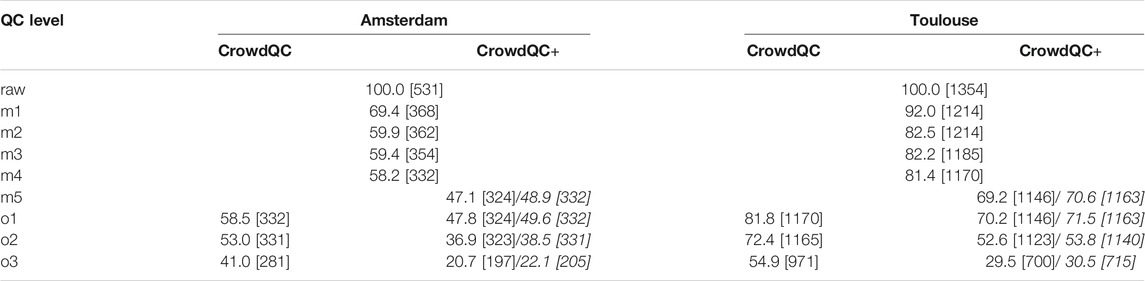
TABLE 3. Percentage of CWS hourly data availability and number of available CWS (given in brackets) at each QC level in Amsterdam (2019) and Toulouse (2020) after application of CrowdQC and CrowdQC+ in their respective default settings (cf. Table 2). Values for CrowdQC+ for QC levels m5 to o3 are given with isolated stations in QC level m5 removed (first values per field) and retained (second values per field, italic).

Figure 4 shows mean ta differences between CWS and PRWS along annual and diurnal cycles in 2019 with the stations grouped by LCZ type. Across all LCZ a distinctive pattern is visible, which is related to the diurnal cycles of ta and incoming shortwave radiation. Higher differences are generally found after midday during the months April to September with highest differences in the late afternoon in summer, while for other times differences are generally lower and consistent. The CWS data set is thus likely still influenced by radiative errors induced by the design of the Netatmo CWS without a proper radiation shield and the setup of CWS in unshaded locations, leading to these higher differences. This might impair analyses of daytime ta conditions in cities when absolute values are of relevance, yet might be of lower relevance when calculating spatial differences among (groups of) CWS, as in, e.g., UHI analyses. Night-time differences are lower and consistent both in time (along annual cycle) and space (across LCZ types), underlining the high applicability of Netatmo CWS in urban climate investigations that focus on night-time. Other types of CWS might be less influenced by radiative errors during daytime due to a better design with lamella-type radiation shields and would thus allow for more reliable daytime analyses. Yet, they might show other deficiencies such as a systematic bias or a sensor drift over time, which have not been observed for Netatmo CWS (Meier et al., 2017; Fenner 2020).

FIGURE 4

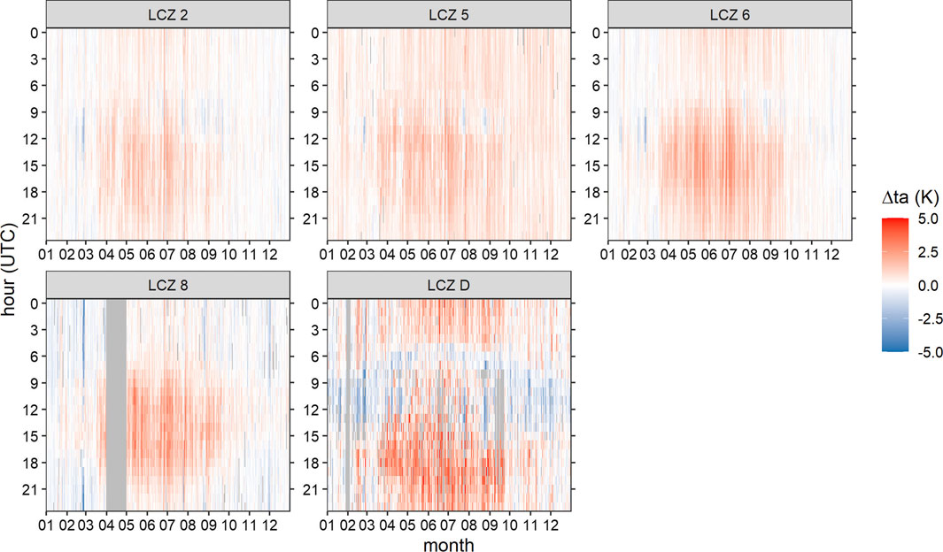
FIGURE 4. Hourly air-temperature difference (∆ta) between mean CWS and mean PRWS ta in Amsterdam per Local Climate Zone LCZ during 2019. CWS data at QC level m5 after CrowdQC+ with default settings (cf. Table 2). CWS and PRWS data were averaged across all stations in the respective LCZ. Missing episodes are displayed in grey.

LCZ D displays a different pattern with higher deviations during night-time and late afternoon and negative differences during winter, spring, and autumn months during daytime (Figure 4). This pattern resembles typical urban heat island characteristics along annual and diurnal cycles (compare, e.g., Fenner et al., 2014; Skarbit et al., 2017). This could indicate that the CWS in LCZ D in Amsterdam contain an “urban” signal in their ta data (due to a set up close to buildings, compared to the PRWS in LCZ D, Schiphol airport. Note though that this PRWS is likely also not completely uninfluenced by man-made surfaces, considering its setup on the airport ground between runways. Another possible reason for this pattern could be related to advective effects. While Schiphol airport is located upwind of Amsterdam (most south-western PRWS in Figure 1A, main wind direction along the annual cycle south-west, not shown), most CWS located in LCZ D are located downwind of built-up areas. Advection of warm air from cities to the surroundings has been reported by observational (e.g., Brandsma et al., 2003; Bassett et al., 2016, 2017) and modelling studies (e.g., Zhang et al., 2012; Heaviside et al., 2015; Bassett et al., 2019).

For Toulouse, mean ta differences between CWS and PRWS along annual and diurnal cycles in 2020 per LCZ type show a different pattern with higher positive deviations during night-time and generally near-zero to negative deviations during daytime (Supplementary Figure S3). To understand these differences, it needs noting that there is a systematic difference in the setup of stations between the CWS and the PRWS network. While CWS are likely located in all kinds of settings, ranging from setups close to building walls and within street canyons to more open settings in residential gardens, the majority of PRWS is located in open areas with little shade. This difference in the setup leads to two possible effects, likely both acting at the same time, which could explain the pattern found. Firstly, ta conditions are different at the sites. CWS located in street canyons and shaded environments experience less radiative heating of the air during daytime than open areas where the PRWS are set up and thus measure lower ta. During night-time, due to reduced sky view factors (SVF) at CWS sites compared to the more open PRWS sites, cooling of the air is hindered, leading to higher ta. This is similar to the first hypothesis brought forward above to explain the deviation for LCZ D in Amsterdam (Figure 4). Secondly, radiative errors contribute to the deviations. Even though the PRWS are of much higher quality than the CWS, especially regarding the station design (Netatmo CWS with aluminium shell around the sensor with little ventilation, Davis Vantage Pro with lamella-type radiation shield, naturally ventilated), the type of PRWS used is not free of radiative errors (Cornes et al., 2020). Comparing the radiation biases of two Davis Vantage Pro with natural ventilation, one in a rural setting with relatively unobstructed airflow and one in a more enclosed residential setting, Cornes et al. (2020) found that measurements at the site in the residential setting experienced radiative errors of >1 K during midday and the warmer months of the year, compared to ≤0.6 K at the rural site. It was suggested that this difference is due to increased airflow at the rural site that aided the ventilation of the radiation screen, reducing radiative errors.

Based on these results and since the majority of PRWS in Toulouse are located in urban, yet open settings with little shading, radiative errors can be expected. On the other hand, radiative errors in the CWS data set should largely be reduced by the QC. Further, hypothesising that the majority of CWS is located in shaded environments, the network of quality-controlled CWS contains less radiative errors during daytime which could then, in the end, lead to the deviations that were found (Supplementary Figure S3). Positive deviations between CWS and PRWS ta for Toulouse during night-time might also be linked to differences in setup. At locations close to building walls, where CWS are typically installed, ta might be higher during night-time than further away from the wall, yet predominantly for walls that were exposed to solar radiation during the day (Nakamura and Oke 1988). The hypotheses brought forward require further systematic investigations, yet go beyond the scope of this study.

Note that all displayed deviations between CWS and PRWS are not all errors of the CWS data set with respect to the PRWS data. Firstly, variation in ta can be expected in the 2000 m radius around each PRWS (used in the calculations of the deviations), even if located in the same LCZ type as the PRWS. Secondly, deviations in ta are likely due to differences in the setup of stations. CWS are typically installed closer to buildings than PRWS, leading to differences in exposure and micro-scale settings at each site, which affect ta (Chapman et al., 2017; Fenner et al., 2017).

Effect of Different Durations

In QC levels m3, m4, and o3 different durations can be defined in the filter applications. To investigate their influence on overall ta deviations, six experiments were run, applying durations from 3 days to the complete data set (1 year) (Table 4, Supplementary Table S1). Overall, differences in deviations between the experiments are small, indicating a robust behaviour of the QC regarding this parameter. When looking at the best results per metric and variable (bold numbers in Table 4 and Supplementary Table S1), choosing the complete data set shows generally best performance. However, using the complete data set at QC level o3 for a 1-year data set reduces final data availability to about 13% of hourly data (compared to the raw data) from 58 CWS in Amsterdam and to nearly 15% from 157 CWS in Toulouse. This is mainly due to QC level o3, checking for data availability per station for the specified duration and flagging a complete station with FALSE in case of not enough valid values (default: fraction of 0.8, i.e., 80% data availability). With marginally higher deviations, but retaining a much higher fraction of data after QC, the use of a shorter duration could be advisable (Table 4, Supplementary Table S1). Based on the obtained results, we recommend to use a duration between 7 days and 1 month. Shorter durations, one the one hand, lead to less robust correlations in QC level m4 with hourly data (sample size at best 72), leading to overall higher deviations. Longer deviations, on the other hand, lead to much more data being excluded, with only a marginal benefit in terms of deviations to PRWS data.

TABLE 4

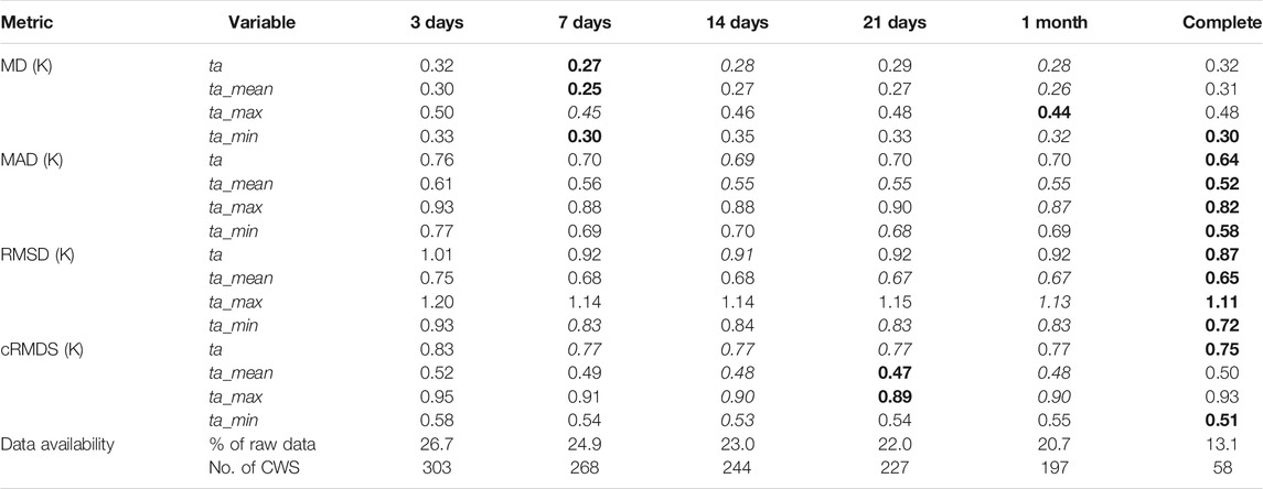
TABLE 4. Mean annual deviations in hourly air temperature (ta) and in aggregated daily values of mean (ta_mean), maximum (ta_max), and minimum (ta_min) between CWS and PRWS in Amsterdam, and remaining data availability during 2019 after applying CrowdQC+ in its default setting (cf. Table 2). Displayed are values at QC level o3 with different “durations” (in QC levels m3, m4, o3). Bold values mark best results per metric and variable, italic values second best. Deviations were calculated between each PRWS and each CWS within a radius of 2000 m around the respective PRWS, located in the same LCZ type as the PRWS. Deviations were then averaged across all CWS and PRWS. MD, mean deviation; MAD, mean absolute deviation; RMSD, root-mean-square deviation; cRMSD, centred RMSD.

Setting parameter “complete = TRUE” is especially useful in cases when only a shorter period of time is under investigation. Further, it could be useful in near-real time applications, when data shall be quality-controlled and used in operational weather monitoring. In such a case, the user could provide data for the past, e.g., 14 days to the QC and use this complete data set for the QC.

Effect of Different Distribution Functions in m2

To test the effect of using the normal distribution or the Student-t distribution when calculating the critical cut-off values in QC level m2, the following experiment was run. After applying QC level m1 and removing all CWS that only provide invalid data after this QC level for each city’s investigation period, a bootstrap approach was chosen to randomly select a subsample of a specified number of CWS from each city’s data set. Then, QC level m2 was carried out, once assuming the normal distribution (parameter “t_distribution = FALSE,” default in cqcp_m2) and once assuming the Student-t distribution (parameter “t_distribution = TRUE”). Afterwards, deviations between CWS and PRWS at QC level m2 were calculated for both data sets for the whole investigation period as described at the end of Statistics section. Finally, deviations were averaged across the number of bootstraps (n = 100). Seven subsample sizes were chosen in the experiment: 10, 25, 50, 100, 150, 200, and 250.

Figure 5 displays the results of the experiment for both cities. Deviations are highest when ten CWS were randomly selected in the bootstrap runs in both cities. With a higher number of CWS, deviations are lower and relatively similar when comparing the sample sizes. For both distribution functions deviations are overall similar when ≥100 CWS were selected. Generally, deviations are lower for the assumption of a normal distribution. Differences in deviations between the two distributions are small but more distinct for a low number of CWS (≤50 CWS, Figure 5).

FIGURE 5

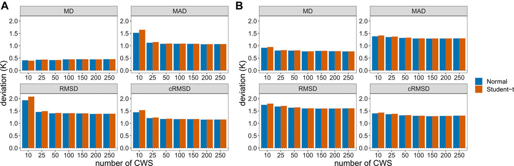
FIGURE 5. Mean annual deviations in hourly air temperature (ta) between CWS and PRWS in (A) Amsterdam during 2019 and (B) Toulouse during 2020 after QC level m2 for subsamples of the CWS data set. Subsamples were randomly selected after QC level m1 in a bootstrap experiment (n = 100). Deviations were calculated per bootstrap run between each PRWS and each CWS within a radius of 2000 m around the respective PRWS, located in the same LCZ type as the PRWS. Deviations were then averaged across all CWS and PRWS, the whole investigation period of each city (cf. Table 1) and all bootstraps. MD, mean deviation; MAD, mean absolute deviation; RMSD, root-mean-square deviation; cRMSD, centred RMSD.

These results firstly show the robustness of QC level m2 to the underlying assumption of distribution for a range of CWS sample sizes. Secondly, it shows that even for CWS networks with a relatively low number of stations per city such as 50–100 CWS, CrowdQC+ yields comparable deviations in the quality-controlled data set compared to networks with more CWS. This highlights the applicability of CrowdQC+ for cities with different CWS network sizes/densities. The fact that assuming a Student-t distribution for the calculation of cut-off values in QC level m2 leads to higher deviations, particularly for low number of CWS, can be explained by the fact that the Student-t distribution assumes heavier tails than the normal distribution. This leads to lower (higher) critical Z-scores for the lower (upper) tail of the distribution, which in turn leads to less values being excluded in QC level m2 when assuming a Student-t distribution.

Based on the results, we suggest to apply the Student-t distribution in QC level m2 if data sets of <100 stations are checked. Considering the statistical hypothesis behind this QC level, the use of the Student-t distribution leads to statistically more robust cut-off values. As a side effect, it will lead to less values being excluded from the already small data set.

Buddy Check

To illustrate the effect of the buddy check in QC level m5, Figure 6 and Supplementary Figure S4 exemplarily display the ta distribution in Amsterdam and Toulouse, respectively, for a day- and night-time situation during a hot summer day. Both figures show that those values that deviate too much from the stations in the immediate surroundings are identified and removed in QC level m5. Additionally, isolated sites are identified and removed, as their quality cannot be assessed due to the lack of available neighbours. In regions where the CWS data set is heterogeneous, the filter retains all values. Here, the ta distribution within the radius is wide and none of the values can be considered a statistical outlier.

FIGURE 6

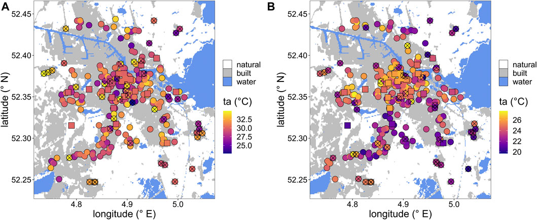
FIGURE 6. Air-temperature (ta) distribution in Amsterdam for (A) June 29, 2019 13:00 UTC and (B) June 30, 2019 01:00 UTC as measured by CWS (circles) and PRWS (squares). CWS data are displayed at QC level m4, crosses mark values that were removed in QC level m5 (radius: 3000 m, minimum number of buddies: 5, alpha: 0.1). Note the different colour scales in the two subplots. Underlying landcover derived from the LCZ map (natural: LCZ A-F, built: LCZ 1-10, water: LCZ G).

In order to highlight the effect of QC level m5 for longer periods of time, Figures 7, 8 display data for Amsterdam for the whole year 2019 (cf. Supplementary Figures S5, S6 for Toulouse). Figure 7 displays scatter plots between PRWS and CWS ta at levels m4 and m5. At the individual PRWS level (Figures 7A,B), as well as considering the whole network of stations (Figures 7C,D), deviations between PRWS and CWS are reduced in all four statistical metrics after QC level m5. Deviations after applying QC level m5 are especially lower for daily maximum ta (Figure 7), compared to daily mean, daily minimum, and hourly ta (all not shown). Hence, higher ta in CWS data during daytime, likely resulting from radiative errors, are now better filtered with the new spatial buddy check. Summarizing, using information from neighbouring CWS to filter likely faulty values in the whole data set is beneficial, also highlighted by others (e.g., de Vos et al., 2019; Båserud et al., 2020; Nipen et al., 2020; Chen et al., 2021).

FIGURE 7

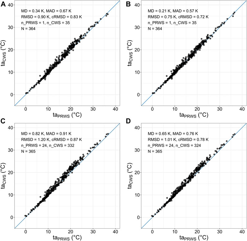
FIGURE 7. Relation between daily maximum air temperature (ta) at PRWS and CWS in Amsterdam during 2019. (A) and (B) for one PRWS (station “2229”; 52.3719°N, 4.89568°E) and the mean of all CWS within a 2000 m radius around the PRWS in the same LCZ type (2–compact midrise). (C) and (D) as the mean across all PRWS and all CWS. (A) and (C) display CWS ta at QC level m4, (B) and (D) CWS ta at QC level m5. MD, mean deviation; MAD, mean absolute deviation; RMSD, root-mean-square deviation; cRMSD, centred RMSD; n_PRWS, number of PRWS; n_CWS, number of CWS; N, number of daily values.

FIGURE 8

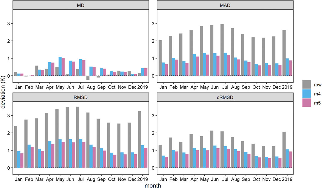
FIGURE 8. Deviations of hourly air temperature (ta) between CWS and PRWS in Amsterdam during 2019 per month and for the whole year for raw data, QC levels m4, and m5. Deviations were calculated between each PRWS and each CWS within a radius of 2000 m around the respective PRWS, located in the same LCZ type as the PRWS. Deviations were then averaged per month and year across all CWS and PRWS. MD, mean deviation; MAD, mean absolute deviation; RMSD, root-mean-square deviation; cRMSD, centred RMSD.

Figure 8 further highlights that the improvement in the statistical metrics is consistently found along the annual cycle, with strongest improvement in the warmer months of the year (April-August), when deviations are higher compared to the rest of the months. Overall, MD is approximately 1 K during summer and <0.3 K during winter at QC levels m4 and m5, being within the specified accuracy of the Netatmo sensor (Meier et al., 2017). For Toulouse, MD is relatively constant throughout the year and always <1 K (Supplementary Figure S5). MAD and RMSD are higher, yet ≤1.5 K after QC level m5 in all months. cRMSD shows that the unsystematic deviation between CWS and PRWS is between 0.6 and 1.3 K in the monthly means after QC level m5 in Amsterdam and Toulouse. Annual averages show that mean CWS ta data on a city scale is ∼0.5 and ∼0.8 K higher than PRWS data after the main QC levels for Amsterdam and Toulouse, respectively (Figure 8, Supplementary Figure S6).

In its current form, the buddy check neglects any spatial gradient in ta in its calculations. Within cities, horizontal gradients in ta might arise in particular from elevation differences among stations on mountain slopes or due to differences in land cover/land use. While the former is addressed in CrowdQC+ with the height correction being carried out, plus the additional check for elevation differences among buddies, the latter is difficult to implement without additional information on underlying surface characteristics. Here, the concept of LCZs might be a suitable candidate to characterise a station in terms of its local surroundings. Such an (optional) addition could be a further extension of CrowdQC+ in the future, yet requires in-depths investigations and might impair subsequent LCZ-based analyses. Per default, a radius of 3000 m is used in QC level m5, which is based on tests for the two investigated cities (not shown) and similar to recommendations by Båserud et al. (2020). In cities with heterogeneous surface cover and morphology, a smaller radius might be more appropriate, as ta will hence be “patchier,” especially during dry, cloud-free, and calm conditions that promote spatial ta gradients (e.g., Parry 1956; Oke 1973; Erell and Williamson 2007; van Hove et al., 2015; Arnds et al., 2017; Fenner et al., 2017; Beck et al., 2018a). Analogously, for urban regions with extensive and homogeneous surface cover and morphology, a larger radius could be applied.

The buddy check is the computationally most expensive of the QC levels. For data sets from several hundred or few thousands of CWS and for extended periods of time such as a year (as in this study), this filter might take several minutes. For near-real time applications such as operational ta monitoring at (half-)hourly resolution this would not be an issue, if a data set of the past, e.g., 14 days is used to perform the complete QC. Further developments of CrowdQC+ will focus on the improvement of this QC level in order to reduce the time spent to perform the buddy check.

Time-Constant Correction

Büchau (2018) determined τ of the Netatmo sensor (investigating in total seven Netatmo stations) by conducting cooldown and warmup tests in a laboratory environment. He determined a mean τ across the sensors of 22.46 and 26.89 min for the two experiments, respectively (Figure 2.3 a and b in Büchau 2018). Based on these results, we apply a mean of these two values in the time-constant correction, using τ = 1480.5 s. The effect of the time-constant correction is illustrated in the following.

Comparison Measurements With One Netatmo Sensor

Firstly, we investigate data from a 1-year long comparison measurement in Berlin in 2015 between one Netatmo sensor and a reference sensor (Campbell Scientific CS215, accuracy ±0.4 K in range 5–40°C). Both sensors were set up at 2 m above ground level, the Netatmo sensor inside a wooden Stevenson Screen, the reference sensor inside a small lamella-type radiation shield, actively ventilated during sunlit periods (Figure 9A). Netatmo data was collected at the original 5-min resolution (approximately) from the user interface of Netatmo, reference data was sampled at 1-min resolution. This data set was previously used in the study by Meier et al. (2017). Figure 9B shows a distinct diurnal cycle in the mean deviation between the two sensors. While in the morning hours after sunrise the Netatmo sensor displays lower mean values than the reference sensor, it shows higher values in the early afternoon.

FIGURE 9

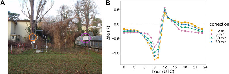
FIGURE 9. (A) Setup of the comparison measurements between one Netatmo CWS, fixed in a wooden Stevenson Screen (purple) and a reference sensor (orange) in Berlin at site Rothenburg (52.4572°N, 13.3158°E) during 2015. (B) Mean diurnal cycle of air-temperature difference (∆ta) between the Netatmo outdoor module and the reference sensor during 2015. The yellow line (squares) corresponds to the mean data as shown by Meier et al. (2017). Netatmo data at the original temporal resolution (∼5 min) was corrected using a time-constant value of 1480.5 s and the formula in Optional Quality-Control Levels section. The correction was applied at different temporal resolutions (original/5, 30, 60 min). Afterwards, all data were aggregated to hourly mean values and the hourly mean values of the PRWS subtracted.

Figure 9B further shows the benefit of applying the time-constant correction (τ = 1480.5 s) to the Netatmo data. If the correction is applied at the original temporal resolution of the Netatmo sensor, the correction reduces the mean hourly deviation in the morning hours by 0.5 K, yet increases the deviation at noon by 0.2 K. The correction further leads to a more “stable” deviation between the two sensors during afternoon and night-time hours at approximately −0.3 K, likely showing a systematic bias. The remaining stronger mean negative and positive deviations in the morning and at noon, respectively, are likely partly due to the slower thermal response of the Stevenson Screen (Bryant 1968; Brandsma and van der Meulen 2008; Harrison 2010) in which the Netatmo sensor was placed, compared to the small lamella-type radiation shield of the reference sensor (actively ventilated during sunlit times).

When using the Netatmo API, different temporal resolutions for obtaining the data can be specified, ranging from the original resolution at approximately 5 min, over 30 and 60 min to 3 h, 1 day, 1 week, or 1 month (https://dev.netatmo.com/apidocumentation/weather#getmeasure). Thus, Figure 9B also displays the effect of the time-constant correction applied at 30- and 60-min data. For this, the original Netatmo data was aggregated to mean values for the respective temporal resolution prior to correction. With decreasing temporal resolution, the effect of the time-constant correction also decreases.

While for hourly resolution the time-constant correction provides only a marginal difference, it is worthwhile to apply in temporally higher-resolution data of the Netatmo sensor and likely also other sensors with similarly large time constants.

Effects in City-Wide Data

Secondly, applying the time-constant correction to the hourly data set in Amsterdam and Toulouse, minor to no differences between the corrected and uncorrected data set with respect to the statistical metrics are found (Supplementary Table S2). For daily maximum ta the time-constant correction leads to higher deviations, while for daily minimum ta overall lower deviations are found. Statistical metrics for daily mean and hourly ta are not affected.

In its current form, QC level o4 assumes the same value for τ for all CWS and hence only works meaningfully with one type of CWS in the data set. A possible future development of CrowdQC+ and improvement of this QC level could be to include information on the type of CWS, thus enabling the correction of different types of CWS with regard to sensor lag in the same data set.

Applications of the Quality-Controlled Data

To highlight the usability of quality-controlled CWS data for urban climate studies, two applications are put forward.

In the first application, the annual and diurnal cycle in ta difference (∆ta) between two LCZ types is displayed for Amsterdam, comparable to typical UHI analyses. Figure 10 displays ∆ta between LCZ 2, as the mean across the quality-controlled CWS (Figure 10A) and across PRWS data (Figure 10B), and the Schiphol airport PRWS. We follow the approach by de Vos et al. (2020) and use the airport station as the “rural” reference for both networks, acknowledging that this is not a true rural reference site. Both sub-figures show the characteristic cycles in ∆ta between urban and rural environments that is found for mid-latitude cities, i.e., higher values during night-time and the warmer months of the year, and lower values during daytime (Oke et al., 2017). Yet, distinctive episodes with higher and lower ∆ta than this typical pattern are also found (visible in the vertical stripe-like pattern), being related to the specific weather conditions during this year. Two of such “stripes” are particularly prominent in the second half of February 2019 with large positive ∆ta during night-time, being episodes of unusually high ta in Amsterdam with clear skies and no precipitation (not shown). Such conditions promote distinct local-scale ∆ta (e.g., Parry 1956; Oke 1973; Erell and Williamson 2007; van Hove et al., 2015; Arnds et al., 2017; Fenner et al., 2017; Beck et al., 2018a) Finally, Figure 10 highlights the strong agreement between both networks when comparing both sub-figures. This underlines the suitability of CWS data for quasi-climatological analyses, if a multitude of quality-controlled CWS are available.

FIGURE 10

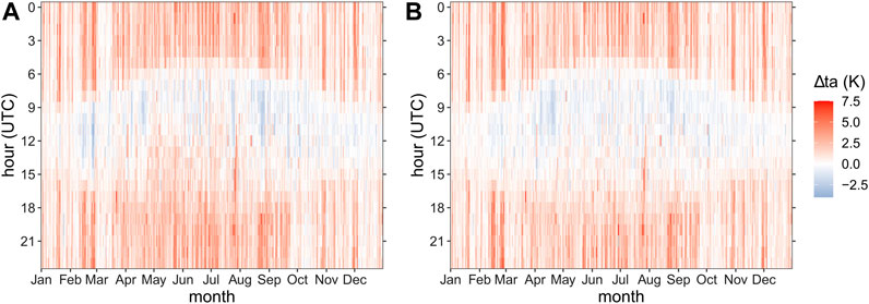
FIGURE 10. Hourly air-temperature difference (∆ta) for Amsterdam between (A) all CWS in LCZ 2 (compact midrise) and (B) all PWRS in LCZ 2, and PRWS at Schiphol airport, LCZ D (low plants) during 2019 (∆ta_{LCZ 2–LCZ D}). CWS data are displayed at QC level o3 after application of CrowdQC+ in default settings (cf. Table 2). CWS and PRWS data for LCZ 2 were first averaged across stations, then data at Schiphol airport subtracted.

In the second application (Figure 11), night-time ta distribution for the month of July 2020 is displayed for Toulouse. July 2020 was a month with heatwave-like conditions and only marginal rain. Figure 11 shows a distinct night-time UHI for Toulouse of several K in the monthly mean, both for CWS and PRWS data. Highest ta was recorded in central districts of Toulouse with generally decreasing ta towards the outskirts and rural areas, comparable to model results from Kwok et al. (2019). Further, the systematic difference between CWS and PRWS data is visible (Figure 11). The application highlights the benefit of using CWS data for mapping of meteorological conditions due to their high density and spatial distribution. Yet, the imbalance between number of CWS in built-up areas and natural settings is also prominent (Chapman et al., 2017; Fenner et al., 2017; Meier et al., 2017; Feichtinger et al., 2020).

FIGURE 11

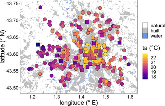
FIGURE 11. Mean air temperature (ta) in Toulouse during July 2020 03:00 UTC as measured by CWS (circles) and PRWS (squares). CWS data are displayed at QC level o3 after application of CrowdQC+ in default settings (cf. Table 2). Underlying landcover derived from the LCZ map (natural: LCZ A-F, built: LCZ 1-10, water: LCZ G).

Conclusion

The availability of CWS data in theoretically every region of the world makes this data source an interesting choice for scientists and practitioners to gain information on atmospheric conditions. This holds even more true for cities, where atmospheric conditions are highly heterogeneous and traditional measurement networks are sparse. Yet, the data come with a number of uncertainties and errors, which require targeted QC procedures.

In this study, the QC package CrowdQC+ was presented, which is a further development of the existing package CrowdQC. CrowdQC+ extends that package and adds several additions and functionalities, i.e., 1) a further QC level for additional spatial filtering to mainly address remaining radiative errors, 2) an option to correct CWS data for slow sensor response, 3) modifications to the existing QC levels to enhance applicability, and 4) additional functionalities for increased user-friendliness. The package is primarily designed to quality-control air-temperature data from CWS. As its predecessor, CrowdQC+ works without any meteorological reference data and can thus be applied in basically every (urban) region with CWS data, enabling large-scale urban climate studies based on CWS data.

Applying CrowdQC+ to two data sets from Netatmo CWS of 1 year for Amsterdam and Toulouse, and comparing the CWS data to data from PRWS, it is shown that CrowdQC+ effectively removes erroneous data and provides an improvement compared to CrowdQC. Deviations between CWS and PRWS data on the city-scale level and per station are lower after applying CrowdQC+ than using CrowdQC in both investigated cities in all seasons, highlighting the additional value of the newly-introduced functionalities. Yet, deviations between CWS and PRWS data remain, which are likely linked to remaining faulty values not identified by the QC, but also to differences in network designs, sensor qualities, and station setups. The trade-off of the reduced deviations and thus increased QC performance of CrowdQC+ compared to CrowdQC is a lower data availability after applying the QC. It is further shown that CrowdQC+ can be applied to CWS data sets of different size, that data sets of different duration can be quality-controlled, and that the newly added functionalities of the package enable the QC to be applied in operational mode for near-real time applications.

This study aims to be a step ahead in a continuous development and enhancement of the package, retaining the core of the QC, which is the applicability in regions without reference meteorological observations. CrowdQC+ is an open-source tool under active development (https://github.com/dafenner/CrowdQCplus), collaboration and participation in further developments of the package are welcome. Future work could focus on the evaluation of the QC with regard to other variables such as air pressure or humidity, which can also be crowdsourced from CWS. Testing the QC on CWS data sets of, e.g., tropical or desert cities would also be of high value to understand its performance in different background climates. Furthermore, future studies could investigate the performance of the QC when applied to crowdsourced data sets composed of measurements by different types of CWS.

Data Availability Statement

CrowdQC+ v1.0.0, as described in this paper, is available as an R package as Supplementary Material. The latest version of CrowdQC+ and the possibility to submit issues is available at https://github.com/dafenner/CrowdQCplus. Publicly available datasets were analyzed in this study. This data can be found here: Netatmo CWS data can freely be obtained via the company’s API at https://dev.netatmo.com/. SRTM digital elevation data is freely available at https://srtm.csi.cgiar.org. PRWS data for Toulouse is freely available at https://data.toulouse-metropole.fr/explore/dataset/stations-meteo-en-place/table/. PRWS data for Amsterdam from the AAMS are available upon request from Gert-Jan Steeneveld or Bert Heusinkveld at Wageningen University & Research. Data from the KNMI can freely be obtained at https://dataplatform.knmi.nl/.

Author Contributions

All authors designed the study. JK, BB, and MD collected the CWS data, DF assembled PRWS data and processed all data used. All authors contributed to the design of the package, DF did the programming of the package. DF carried out all analyses and mainly wrote the manuscript. All authors discussed the results and contributed to the writing of the manuscript.

Funding

This work was conducted in the context of project ENLIGHT, funded by the German Research Foundation (DFG) under grant No. 437467569. The Amsterdam Atmospheric Monitoring Supersite (AAMS) has been financially supported by the Amsterdam Institute for Advanced Metropolitan Solutions (AMS) under grant VIR16002 and the NWO/eScience grant 027.012.103.

Conflict of Interest

The authors declare that the research was conducted in the absence of any commercial or financial relationships that could be construed as a potential conflict of interest.

The reviewer (TC) declared a past co-authorship with one of the authors (BB) to the handling Editor.

Publisher’s Note

All claims expressed in this article are solely those of the authors and do not necessarily represent those of their affiliated organizations, or those of the publisher, the editors and the reviewers. Any product that may be evaluated in this article, or claim that may be made by its manufacturer, is not guaranteed or endorsed by the publisher.

Acknowledgments

We thank all CWS owners who shared their data publicly. Tom Grassmann is thanked for sharing ideas and code in the development of CrowdQC+. We are grateful to Gert-Jan Steeneveld and Bert Heusinkveld at Wageningen University & Research (WUR) for sharing of and support with the PRWS data in Amsterdam. We further thank Guillaume Dumas at the Centre national de la recherche scientifique (CNRS) for support with the PRWS data in Toulouse. We acknowledge the WUDAPT contributors Julia Hidalgo and Ran Wang for providing the LCZ training areas for Toulouse and Amsterdam, respectively.

Supplementary Material

The Supplementary Material for this article can be found online at: https://www.frontiersin.org/articles/10.3389/fenvs.2021.720747/full#supplementary-material

References

Arnds, D., Böhner, J., and Bechtel, B. (2017). Spatio-Temporal Variance and Meteorological Drivers of the Urban Heat Island in a European City. Theor. Appl. Climatol. 128 (1), 43–61. doi:10.1007/s00704-015-1687-4

CrossRef Full Text | Google Scholar

Arnfield, A. J. (2003). Two Decades of Urban Climate Research: a Review of Turbulence, Exchanges of Energy and Water, and the Urban Heat Island. Int. J. Climatol. 23 (1), 1–26. doi:10.1002/joc.859

CrossRef Full Text | Google Scholar

Bárdossy, A., Seidel, J., and El Hachem, A. (2021). The Use of Personal Weather Station Observations to Improve Precipitation Estimation and Interpolation. Hydrol. Earth Syst. Sci. 25, 583–601. doi:10.5194/hess-25-583-2021

CrossRef Full Text | Google Scholar

Båserud, L., Lussana, C., Nipen, T. N., Seierstad, I. A., Oram, L., and Aspelien, T. (2020). TITAN Automatic Spatial Quality Control of Meteorological In-Situ Observations. Adv. Sci. Res. 17, 153–163. doi:10.5194/asr-17-153-2020

CrossRef Full Text | Google Scholar

Bartos, M., Park, H., Zhou, T., Kerkez, B., and Vasudevan, R. (2019). Windshield Wipers on Connected Vehicles Produce High-Accuracy Rainfall Maps. Sci. Rep. 9 (1), 170. doi:10.1038/s41598-018-36282-7

PubMed Abstract | CrossRef Full Text | Google Scholar

Bassett, R., Cai, X., Chapman, L., Heaviside, C., Thornes, J. E., Muller, C. L., et al. (2016). Observations of Urban Heat Island Advection from a High-Density Monitoring Network. Q.J.R. Meteorol. Soc. 142 (699), 2434–2441. doi:10.1002/qj.2836

CrossRef Full Text | Google Scholar

Bassett, R., Cai, X., Chapman, L., Heaviside, C., and Thornes, J. E. (2017). The Effects of Heat Advection on UK Weather and Climate Observations in the Vicinity of Small Urbanized Areas. Boundary-layer Meteorol. 165 (1), 181–196. doi:10.1007/s10546-017-0263-0

PubMed Abstract | CrossRef Full Text | Google Scholar

Bassett, R., Cai, X., Chapman, L., Heaviside, C., and Thornes, J. E. (2019). Semi-idealized Urban Heat Advection Simulations Using the Weather Research and Forecasting Mesoscale Model. Int. J. Climatol. 39 (3), 1345–1358. doi:10.1002/joc.5885

CrossRef Full Text | Google Scholar

Bechtel, B., Alexander, P., Böhner, J., Ching, J., Conrad, O., Feddema, J., et al. (2015). Mapping Local Climate Zones for a Worldwide Database of the Form and Function of Cities. Ijgi 4, 199–219. doi:10.3390/ijgi4010199

CrossRef Full Text | Google Scholar

Bechtel, B., Alexander, P. J., Beck, C., Böhner, J., Brousse, O., Ching, J., et al. (2019). Generating WUDAPT Level 0 Data - Current Status of Production and Evaluation. Urban Clim. 27, 24–45. doi:10.1016/j.uclim.2018.10.001

CrossRef Full Text | Google Scholar

Bechtel, B., Demuzere, M., and Stewart, I. D. (2020). A Weighted Accuracy Measure for Land Cover Mapping: Comment on Johnson et al. Local Climate Zone (LCZ) Map Accuracy Assessments Should Account for Land Cover Physical Characteristics that Affect the Local Thermal Environment. Remote Sens. 2019, 11, 2420. Remote Sens. 1112 (11), 24201769. doi:10.3390/rs12111769

CrossRef Full Text | Google Scholar

Beck, C., Straub, A., Breitner, S., Cyrys, J., Philipp, A., Rathmann, J., et al. (2018a). Air Temperature Characteristics of Local Climate Zones in the Augsburg Urban Area (Bavaria, Southern Germany) under Varying Synoptic Conditions. Urban Clim. 25, 152–166. doi:10.1016/j.uclim.2018.04.007

CrossRef Full Text | Google Scholar

Beck, H. E., Zimmermann, N. E., McVicar, T. R., Vergopolan, N., Berg, A., and Wood, E. F. (2018b). Present and Future Köppen-Geiger Climate Classification Maps at 1-km Resolution. Sci. Data 5 (1), 180214. doi:10.1038/sdata.2018.214

PubMed Abstract | CrossRef Full Text | Google Scholar

Bell, S., Cornford, D., and Bastin, L. (2013). The State of Automated Amateur Weather Observations. Weather 68 (2), 36–41. doi:10.1002/wea.1980

CrossRef Full Text | Google Scholar

Bell, S., Cornford, D., and Bastin, L. (2015). How Good Are Citizen Weather Stations? Addressing a Biased Opinion. Weather 70 (3), 75–84. doi:10.1002/wea.2316

CrossRef Full Text | Google Scholar

Bell, S. J. (2015). Quantifying Uncertainty in Citizen Weather Data. Birmingham, United Kingdom: Aston University. PhD Thesis.

Google Scholar

Benjamin, K., Luo, Z., and Wang, X. (2021). Crowdsourcing Urban Air Temperature Data for Estimating Urban Heat Island and Building Heating/Cooling Load in London. Energies 14 (16), 5208. doi:10.3390/en14165208

CrossRef Full Text | Google Scholar

Brandsma, T., and van der Meulen, J. P. (2008). Thermometer Screen Intercomparison in De Bilt (the Netherlands)-Part II: Description and Modeling of Mean Temperature Differences and Extremes. Int. J. Climatol. 28 (3), 389–400. doi:10.1002/joc.1524

CrossRef Full Text | Google Scholar

Brandsma, T., Können, G. P., and Wessels, H. R. A. (2003). Empirical Estimation of the Effect of Urban Heat Advection on the Temperature Series of De Bilt (The Netherlands). Int. J. Climatol. 23 (7), 829–845. doi:10.1002/joc.902

CrossRef Full Text | Google Scholar

Bryant, D. (1968). An Investigation into the Response of Thermometer Screens - the Effect of Wind Speed on the Lag Time. Meteorol. Mag. 97, 183–186.

Google Scholar

Büchau, Y. G. (2018). Modelling Shielded Temperature Sensors - an Assessment of the Netatmo Citizen Weather Station. MSc Thesis, Universität Hamburg. Available at: https://bis-erdsystem.de/fileadmin/user_upload/bise/Texte/MSC_Met_61-20180313.pdf. (Accessed November 12, 2021).

Google Scholar

Cerlini, P. B., Silvestri, L., and Saraceni, M. (2020). Quality Control and gap‐filling Methods Applied to Hourly Temperature Observations over central Italy. Meteorol. Appl. 27 (3), e1913. doi:10.1002/met.1913

CrossRef Full Text | Google Scholar

Chapman, L., Muller, C. L., Young, D. T., Warren, E. L., Grimmond, C. S. B., Cai, X.-M., et al. (2015). The Birmingham Urban Climate Laboratory: An Open Meteorological Test Bed and Challenges of the Smart City. Bull. Am. Meteorol. Soc. 96, 1545–1560. doi:10.1175/BAMS-D-13-00193.1

CrossRef Full Text | Google Scholar

Chapman, L., Bell, C., and Bell, S. (2017). Can the Crowdsourcing Data Paradigm Take Atmospheric Science to a New Level? A Case Study of the Urban Heat Island of London Quantified Using Netatmo Weather Stations. Int. J. Climatol. 37 (9), 3597–3605. doi:10.1002/joc.4940

CrossRef Full Text | Google Scholar

Chen, J., Saunders, K., and Whan, K. (2021). Quality Control and Bias Adjustment of Crowdsourced Wind Speed Observations. QJR Meteorol. Soc. 147, 3647–3664. doi:10.1002/qj.4146

CrossRef Full Text | Google Scholar

Ching, J., Mills, G., Bechtel, B., See, L., Feddema, J., Wang, X., et al. (2018). World Urban Database and Access Portal Tools (WUDAPT), an urban weather, climate and environmental modeling infrastructure for the Anthropocene. Bull. Am. Meteorol. Soc. 99, 1907–1924. doi:10.1175/bams-d-16-0236.1

CrossRef Full Text | Google Scholar

Chwala, C., and Kunstmann, H. (2019). Commercial Microwave Link Networks for Rainfall Observation: Assessment of the Current Status and Future Challenges. WIREs Water 6 (2), e1337. doi:10.1002/wat2.1337

CrossRef Full Text | Google Scholar

Clark, M. R., Webb, J. D. C., and Kirk, P. J. (2018). Fine-scale Analysis of a Severe Hailstorm Using Crowd-Sourced and Conventional Observations. Met. Apps 25 (3), 472–492. doi:10.1002/met.1715

CrossRef Full Text | Google Scholar

Cornes, R. C., Dirksen, M., and Sluiter, R. (2020). Correcting Citizen‐science Air Temperature Measurements across the Netherlands for Short Wave Radiation Bias. Meteorol. Appl. 27, e1814. doi:10.1002/met.1814

CrossRef Full Text | Google Scholar

de Vos, L., Leijnse, H., Overeem, A., and Uijlenhoet, R. (2017). The Potential of Urban Rainfall Monitoring with Crowdsourced Automatic Weather Stations in Amsterdam. Hydrol. Earth Syst. Sci. 21 (2), 765–777. doi:10.5194/hess-21-765-2017

CrossRef Full Text | Google Scholar

de Vos, L. W., Leijnse, H., Overeem, A., and Uijlenhoet, R. (2019). Quality Control for Crowdsourced Personal Weather Stations to Enable Operational Rainfall Monitoring. Geophys. Res. Lett. 46 (15), 8820–8829. doi:10.1029/2019gl083731

CrossRef Full Text | Google Scholar

de Vos, L. W., Droste, A. M., Zander, M. J., Overeem, A., Leijnse, H., Heusinkveld, B. G., et al. (2020). Hydrometeorological Monitoring Using Opportunistic Sensing Networks in the Amsterdam Metropolitan Area. Bull. Am. Meteorol. Soc. 101, E167–E185. doi:10.1175/bams-d-19-0091.1

CrossRef Full Text | Google Scholar

Demuzere, M., Bechtel, B., Middel, A., and Mills, G. (2019a). Mapping Europe into Local Climate Zones. PLoS One 14 (4), e0214474. doi:10.1371/journal.pone.0214474

PubMed Abstract | CrossRef Full Text | Google Scholar

Demuzere, M., Bechtel, B., and Mills, G. (2019b). Global Transferability of Local Climate Zone Models. Urban Clim. 27, 46–63. doi:10.1016/j.uclim.2018.11.001

CrossRef Full Text | Google Scholar

Demuzere, M., Hankey, S., Mills, G., Zhang, W., Lu, T., and Bechtel, B. (2020). Combining Expert and Crowd-Sourced Training Data to Map Urban Form and Functions for the continental US. Sci. Data 7, 264. doi:10.1038/s41597-020-00605-z

PubMed Abstract | CrossRef Full Text | Google Scholar

Demuzere, M., Kittner, J., and Bechtel, B. (2021). LCZ Generator: A Web Application to Create Local Climate Zone Maps. Front. Environ. Sci. 9, 637455. doi:10.3389/fenvs.2021.637455

CrossRef Full Text | Google Scholar

Dowle, M., and Srinivasan, A. (2021). data.table: Extension of `data.Frame`. R package version 1.13.0. Available at: https://CRAN.R-project.org/package=data.table. (Accessed November 12, 2021).

Google Scholar

Droste, A. M., Pape, J. J., Overeem, A., Leijnse, H., Steeneveld, G. J., Van Delden, A. J., et al. (2017). Crowdsourcing Urban Air Temperatures through Smartphone Battery Temperatures in São Paulo, Brazil. J. Atmos. Ocean. Tech. 34 (9), 1853–1866. doi:10.1175/JTECH-D-16-0150.1

CrossRef Full Text | Google Scholar

Droste, A. M., Heusinkveld, B. G., Fenner, D., and Steeneveld, G. J. (2020). Assessing the Potential and Application of Crowdsourced Urban Wind Data. QJR Meteorol. Soc. 146 (731), 2671–2688. doi:10.1002/qj.3811

CrossRef Full Text | Google Scholar

Erell, E., and Williamson, T. (2007). Intra-urban Differences in Canopy Layer Air Temperature at a Mid-latitude City. Int. J. Climatol. 27, 1243–1255. doi:10.1002/joc.1469

CrossRef Full Text | Google Scholar

Estévez, J., Gavilán, P., and Giráldez, J. V. (2011). Guidelines on Validation Procedures for Meteorological Data from Automatic Weather Stations. J. Hydrol. 402 (1-2), 144–154. doi:10.1016/j.jhydrol.2011.02.031

CrossRef Full Text | Google Scholar

Feichtinger, M., de Wit, R., Goldenits, G., Kolejka, T., Hollósi, B., Žuvela-Aloise, M., et al. (2020). Case-study of Neighborhood-Scale Summertime Urban Air Temperature for the City of Vienna Using Crowd-Sourced Data. Urban Clim. 32, 100597. doi:10.1016/j.uclim.2020.100597

CrossRef Full Text | Google Scholar

Fenner, D., Meier, F., Scherer, D., and Polze, A. (2014). Spatial and Temporal Air Temperature Variability in Berlin, Germany, during the Years 2001-2010. Urban Clim. 10 (2), 308–331. doi:10.1016/j.uclim.2014.02.004

CrossRef Full Text | Google Scholar

Fenner, D., Meier, F., Bechtel, B., Otto, M., and Scherer, D. (2017). Intra and Inter 'local Climate Zone' Variability of Air Temperature as Observed by Crowdsourced Citizen Weather Stations in Berlin, Germany. Meteorol. Z. 26 (5), 525–547. doi:10.1127/metz/2017/0861

CrossRef Full Text | Google Scholar

Fenner, D., Holtmann, A., Meier, F., Langer, I., and Scherer, D. (2019). Contrasting Changes of Urban Heat Island Intensity during Hot Weather Episodes. Environ. Res. Lett. 14 (12), 124013. doi:10.1088/1748-9326/ab506b

CrossRef Full Text | Google Scholar

Fenner, D. (2020). Heatwaves and Urban thermal Climates in Berlin, Germany. Berlin, Germany: Technische Universität Berlin. PhD Thesis. doi:10.14279/depositonce-10378

CrossRef Full Text | Google Scholar

Fiebrich, C. A., Morgan, C. R., McCombs, A. G., Hall, P. K., and McPherson, R. A. (2010). Quality Assurance Procedures for Mesoscale Meteorological Data. J. Atmos. Ocean. Tech. 27 (10), 1565–1582. doi:10.1175/2010JTECHA1433.1

CrossRef Full Text | Google Scholar

Gosset, W. S. (1908). The Probable Error of a Mean. Biometrika 6 (1), 1–25. doi:10.2307/2331554

CrossRef Full Text | Google Scholar

Grassmann, T., Napoly, A., Meier, F., and Fenner, D. (2018). Quality Control for Crowdsourced Data from CWS. (Accessed November 12, 2021). doi:10.14279/depositonce-6740.3

CrossRef Full Text | Google Scholar

Haberlandt, U., and Sester, M. (2010). Areal Rainfall Estimation Using Moving Cars as Rain Gauges - a Modelling Study. Hydrol. Earth Syst. Sci. 14 (7), 1139–1151. doi:10.5194/hess-14-1139-2010

CrossRef Full Text | Google Scholar

Hammerberg, K., Brousse, O., Martilli, A., and Mahdavi, A. (2018). Implications of Employing Detailed Urban Canopy Parameters for Mesoscale Climate Modelling: a Comparison between WUDAPT and GIS Databases over Vienna, Austria. Int. J. Climatol. 38 (S1), e1241–e1257. doi:10.1002/joc.5447

CrossRef Full Text | Google Scholar

Harrison, R. G. (2010). Natural Ventilation Effects on Temperatures within Stevenson Screens. Q.J.R. Meteorol. Soc. 136 (646), 253–259. doi:10.1002/qj.537

CrossRef Full Text | Google Scholar

Heaviside, C., Cai, X. M., and Vardoulakis, S. (2015). The Effects of Horizontal Advection on the Urban Heat Island in Birmingham and the West Midlands, United Kingdom during a Heatwave. Q.J.R. Meteorol. Soc. 141 (689B), 1429–1441. doi:10.1002/qj.2452

CrossRef Full Text | Google Scholar

Hijmans, R. J. (2021). Raster: Geographic Data Analysis and Modeling. R package version 3.3-13. Available at: https://CRAN.R-project.org/package=raster. (Accessed November 12, 2021).

Google Scholar

Jarvis, A., Reuter, H. I., Nelson, A., and Guevara, E. (2008). Hole-filled Seamless SRTM Data V4. International Centre for Tropical Agriculture CIAT. available from: https://srtm.csi.cgiar.org. (Accessed November 12, 2021).

Google Scholar

Kwok, Y. T., Schoetter, R., Lau, K. K. L., Hidalgo, J., Ren, C., Pigeon, G., et al. (2019). How Well Does the Local Climate Zone Scheme Discern the thermal Environment of Toulouse (France)? an Analysis Using Numerical Simulation Data. Int. J. Climatol. 39 (14), 5292–5315. doi:10.1002/joc.6140

CrossRef Full Text | Google Scholar

Langer, I., Fakharizadehshirazi, E., and Werner, J. (2021). Spatial Variation of Physiologically Equivalent Temperature in Different Local Climate Zones of a Large City during a Hot Spell. Meteorol. Z. 30 (2), 115–125. doi:10.1127/metz/2020/0996

CrossRef Full Text | Google Scholar

Lelovics, E., Unger, J., Gál, T., and Gál, C. (2014). Design of an Urban Monitoring Network Based on Local Climate Zone Mapping and Temperature Pattern Modelling. Clim. Res. 60, 51–62. doi:10.3354/cr01220

CrossRef Full Text | Google Scholar

Madaus, L. E., Hakim, G. J., and Mass, C. F. (2014). Utility of Dense Pressure Observations for Improving Mesoscale Analyses and Forecasts. Mon. Weather Rev. 142 (7), 2398–2413. doi:10.1175/mwr-d-13-00269.1

CrossRef Full Text | Google Scholar

Mandement, M., and Caumont, O. (2020). Contribution of Personal Weather Stations to the Observation of Deep-Convection Features Near the Ground. Nat. Hazards Earth Syst. Sci. 20, 299–322. doi:10.5194/nhess-20-299-2020

CrossRef Full Text | Google Scholar

Mass, C. F., and Madaus, L. E. (2014). Surface Pressure Observations from Smartphones: A Potential Revolution for High-Resolution Weather Prediction? Bull. Am. Meteorol. Soc. 95, 1343–1349. doi:10.1175/BAMS-D-13-00188.1

CrossRef Full Text | Google Scholar

Meier, F., Fenner, D., Grassmann, T., Otto, M., and Scherer, D. (2017). Crowdsourcing Air Temperature from Citizen Weather Stations for Urban Climate Research. Urban Clim. 19, 170–191. doi:10.1016/j.uclim.2017.01.006

CrossRef Full Text | Google Scholar

Messer, H., Zinevich, A., and Alpert, P. (2006). Environmental Monitoring by Wireless Communication Networks. Science 312 (5774), 713. doi:10.1126/science.1120034

PubMed Abstract | CrossRef Full Text | Google Scholar

Miloshevich, L. M., Paukkunen, A., Vömel, H., and Oltmans, S. J. (2004). Development and Validation of a Time-Lag Correction for Vaisala Radiosonde Humidity Measurements. J. Atmos. Oceanic Technol. 21 (9), 1305–1327. doi:10.1175/1520-0426(2004)021<1305:davoat>2.0.co;2

CrossRef Full Text | Google Scholar

Muller, C. L., Chapman, L., Grimmond, C. S. B., Young, D. T., and Cai, X. (2013). Sensors and the City: a Review of Urban Meteorological Networks. Int. J. Climatol. 33 (7), 1585–1600. doi:10.1002/joc.3678

CrossRef Full Text | Google Scholar

Muller, C. L., Chapman, L., Johnston, S., Kidd, C., Illingworth, S., Foody, G., et al. (2015). Crowdsourcing for Climate and Atmospheric Sciences: Current Status and Future Potential. Int. J. Climatol. 35 (11), 3185–3203. doi:10.1002/joc.4210

CrossRef Full Text | Google Scholar

Nakamura, Y., and Oke, T. R. (1988). Wind, Temperature and Stability Conditions in an East-West Oriented Urban canyon. Atmos. Environ. (1967) 22 (12), 2691–2700. doi:10.1016/0004-6981(88)90437-4

CrossRef Full Text | Google Scholar

Napoly, A., Grassmann, T., Meier, F., and Fenner, D. (2018). Development and Application of a Statistically-Based Quality Control for Crowdsourced Air Temperature Data. Front. Earth Sci. 6, 118. doi:10.3389/feart.2018.00118

CrossRef Full Text | Google Scholar

Nazarian, N., Liu, S., Kohler, M., Lee, J. K. W., Miller, C., Chow, W. T. L., et al. (2021). Project Coolbit: Can Your Watch Predict Heat Stress and thermal comfort Sensation? Environ. Res. Lett. 16 (3), 034031. doi:10.1088/1748-9326/abd130

CrossRef Full Text | Google Scholar

Nipen, T. N., Seierstad, I. A., Lussana, C., Kristiansen, J., and Hov, Ø. (2020). Adopting Citizen Observations in Operational Weather Prediction. Bull. Amer. Meteorol. Soc. 101, E43–E57. doi:10.1175/bams-d-18-0237.1

CrossRef Full Text | Google Scholar

Oke, T. R., Mills, G., Christen, A., and Voogt, J. A. (2017). Urban Climates. Cambridge, United Kingdom: Cambridge University Press. doi:10.1017/9781139016476

CrossRef Full Text | Google Scholar

Oke, T. R. (1973). City Size and the Urban Heat Island. Atmos. Environ. (1967) 7 (8), 769–779. doi:10.1016/0004-6981(73)90140-6

CrossRef Full Text | Google Scholar

Overeem, A., Leijnse, H., and Uijlenhoet, R. (2013a). Country-wide Rainfall Maps from Cellular Communication Networks. Proc. Natl. Acad. Sci. 110 (8), 2741–2745. doi:10.1073/pnas.1217961110

PubMed Abstract | CrossRef Full Text | Google Scholar

Overeem, A., R. Robinson, J. C., Leijnse, H., Steeneveld, G. J., P. Horn, B. K., and Uijlenhoet, R. (2013b). Crowdsourcing Urban Air Temperatures from Smartphone Battery Temperatures. Geophys. Res. Lett. 40, 4081–4085. doi:10.1002/grl.50786

CrossRef Full Text | Google Scholar

Parry, M. (1956). Local Temperature Variations in the Reading Area. Q.J R. Met. Soc. 82 (351), 45–57. doi:10.1002/qj.49708235105

CrossRef Full Text | Google Scholar

Potgieter, J., Nazarian, N., Lipson, M. J., Hart, M. A., Ulpiani, G., Morrison, W., et al. (2021). Combining High-Resolution Land Use Data with Crowdsourced Air Temperature to Investigate Intra-urban Microclimate. Front. Environ. Sci. 9, 720323. doi:10.3389/fenvs.2021.720323

CrossRef Full Text | Google Scholar

R Core Team (2021). R: A Language and Environment for Statistical Computing. Vienna, Austria: R Foundation for Statistical Computing. URL: https://www.R-project.org/.

Google Scholar

Ronda, R. J., Steeneveld, G. J., Heusinkveld, B. G., Attema, J. J., and Holtslag, A. A. M. (2017). Urban Finescale Forecasting Reveals Weather Conditions with Unprecedented Detail. Bull. Am. Meteorol. Soc. 98 (12), 2675–2688. doi:10.1175/BAMS-D-16-0297.1

CrossRef Full Text | Google Scholar

Rousseeuw, P. J., and Croux, C. (1993). Alternatives to the Median Absolute Deviation. J. Am. Stat. Assoc. 88 (424), 1273–1283. doi:10.1080/01621459.1993.10476408

CrossRef Full Text | Google Scholar

Šećerov, I. B., Savić, S. M., Milošević, D. D., Arsenović, D. M., Dolinaj, D. M., and Popov, S. B. (2019). Progressing Urban Climate Research Using a High-Density Monitoring Network System. Environ. Monit. Assess. 191 (2), 89. doi:10.1007/s10661-019-7210-0

PubMed Abstract | CrossRef Full Text | Google Scholar

Shafer, M. A., Fiebrich, C. A., Arndt, D. S., Fredrickson, S. E., and Hughes, T. W. (2000). Quality Assurance Procedures in the Oklahoma Mesonetwork. J. Atmos. Oceanic Technol. 17 (4), 474–494. doi:10.1175/1520-0426(2000)017<0474:qapito>2.0.co;2

CrossRef Full Text | Google Scholar

Skarbit, N., Stewart, I. D., Unger, J., and Gál, T. (2017). Employing an Urban Meteorological Network to Monitor Air Temperature Conditions in the 'local Climate Zones' of Szeged, Hungary. Int. J. Climatol. 37 (S1), 582–596. doi:10.1002/joc.5023

CrossRef Full Text | Google Scholar

Smiatek, G., Keis, F., Chwala, C., Fersch, B., and Kunstmann, H. (2017). Potential of Commercial Microwave Link Network Derived Rainfall for River Runoff Simulations. Environ. Res. Lett. 12 (3), 034026. doi:10.1088/1748-9326/aa5f46

CrossRef Full Text | Google Scholar

Steeneveld, G. J., Koopmans, S., Heusinkveld, B. G., van Hove, L. W. A., and Holtslag, A. A. M. (2011). Quantifying Urban Heat Island Effects and Human comfort for Cities of Variable Size and Urban Morphology in the Netherlands. J. Geophys. Res. 116 (D20), D20129. doi:10.1029/2011JD015988

CrossRef Full Text | Google Scholar

Stewart, I. D. (2019). Why Should Urban Heat Island Researchers Study History? Urban Clim. 30, 100484. doi:10.1016/j.uclim.2019.100484

CrossRef Full Text | Google Scholar

Stewart, I. D., and Oke, T. R. (2012). Local climate zones for urban temperature studies Bull. Am. Meteorol. Soc. 93 (12), 1879–1900. doi:10.1175/BAMS-D-11-00019.1

CrossRef Full Text | Google Scholar

Taylor, K. E. (2001). Summarizing Multiple Aspects of Model Performance in a Single Diagram. J. Geophys. Res. 106 (D7), 7183–7192. doi:10.1029/2000JD900719

CrossRef Full Text | Google Scholar

van Hove, L. W. A., Jacobs, C. M. J., Heusinkveld, B. G., Elbers, J. A., van Driel, B. L., and Holtslag, A. A. M. (2015). Temporal and Spatial Variability of Urban Heat Island and thermal comfort within the Rotterdam Agglomeration. Build. Environ. 83, 91–103. doi:10.1016/j.buildenv.2014.08.029

CrossRef Full Text | Google Scholar

Varentsov, M., Fenner, D., Meier, F., Samsonov, T., and Demuzere, M. (2021). Quantifying Local- and Meso-Scale Drivers of Moscow’s Urban Heat Island with Reference and Crowdsourced Observations. Frontiers in Environmental Science. doi:10.3389/fenvs.2021.716968

CrossRef Full Text | Google Scholar

Venter, Z. S., Brousse, O., Esau, I., and Meier, F. (2020). Hyperlocal Mapping of Urban Air Temperature Using Remote Sensing and Crowdsourced Weather Data. Remote Sens. Environ. 242, 111791. doi:10.1016/j.rse.2020.111791

CrossRef Full Text | Google Scholar

Venter, Z. S., Chakraborty, T., and Lee, X. (2021). Crowdsourced Air Temperatures Contrast Satellite Measures of the Urban Heat Island and its Mechanisms. Sci. Adv. 7 (22), eabb9569. doi:10.1126/sciadv.abb9569

PubMed Abstract | CrossRef Full Text | Google Scholar

Vulova, S., Meier, F., Fenner, D., Nouri, H., and Kleinschmit, B. (2020). Summer Nights in Berlin, Germany: Modeling Air Temperature Spatially with Remote Sensing, Crowdsourced Weather Data, and Machine Learning. IEEE J. Sel. Top. Appl. Earth Observ. Remote Sens. 13, 5074–5087. doi:10.1109/jstars.2020.3019696

CrossRef Full Text | Google Scholar

Warren, E. L., Young, D. T., Chapman, L., Muller, C., Grimmond, C. S. B., and Cai, X.-M. (2016). The Birmingham Urban Climate Laboratory-A High Density, Urban Meteorological Dataset, from 2012-2014. Sci. Data 3, 160038. doi:10.1038/sdata.2016.38

PubMed Abstract | CrossRef Full Text | Google Scholar

Wolters, D., and Brandsma, T. (2012). Estimating the Urban Heat Island in Residential Areas in the Netherlands Using Observations by Weather Amateurs. J. Appl. Meteorol. Clim. 51 (4), 711–721. doi:10.1175/JAMC-D-11-0135.1

CrossRef Full Text | Google Scholar

Yamazaki, D., Ikeshima, D., Tawatari, R., Yamaguchi, T., O'Loughlin, F., Neal, J. C., et al. (2017). A High-Accuracy Map of Global Terrain Elevations. Geophys. Res. Lett. 44 (11), 5844–5853. doi:10.1002/2017gl072874

CrossRef Full Text | Google Scholar

Zahumenský, I. (2004). Guidelines on Quality Control Procedures for Data from Automatic Weather Stations. Document CIMO/OPAG-SURFACE/ET ST\\&MT-1/Doc.6.1(2). Geneva, Switzerland: World Meteorological Organization.

Google Scholar

Zhang, D.-L., Shou, Y.-X., Dickerson, R. R., and Chen, F. (2011). Impact of Upstream Urbanization on the Urban Heat Island Effects along the Washington-Baltimore Corridor. J. Appl. Meteorol. Clim. 50 (10), 2012–2029. doi:10.1175/jamc-d-10-05008.1

CrossRef Full Text | Google Scholar

Zumwald, M., Knüsel, B., Bresch, D. N., and Knutti, R. (2021). Mapping Urban Temperature Using Crowd-Sensing Data and Machine Learning. Urban Clim. 35, 100739. doi:10.1016/j.uclim.2020.100739

CrossRef Full Text | Google Scholar