Soil Surface Micro-Topography by Structure-from-Motion Photogrammetry for Monitoring Density and Erosion Dynamics

Introduction

Soil loss due to erosion is a global threat to arable land, environment and agricultural productivity (e.g., Borrelli et al., 2013; Pimentel and Burgess, 2013; Sutton et al., 2016). In order to take effective erosion control measures, it is necessary to quantify the soil mass that has been translocated during erosion (García-Ruiz et al., 2015). Standard approaches include stationary sediment and run-off collectors installed at experimental hillslopes, which can operate automatically for the event-based erosion monitoring (e.g., Deumlich et al., 2017) or temporary rainfall simulation experiments (e.g., Kaiser et al., 2015). Disadvantages of these methods include the cost for installation in case of monitoring stations and the relatively small surveillance areas of rainfall simulators (Boardman, 2006). Recently, the Structure-from-Motion (SfM) photogrammetry has been developed as an alternative method (James and Robson, 2012; Eltner et al., 2016) to generate Digital Elevation Models (DEMs) in relatively high spatial resolution (Eltner et al., 2015). By combining the images taken from several cardinal points after calibration (Westoby et al., 2012), this method allows to even utilize digital images from low-cost consumer-grade cameras such as those in smart-phones (Micheletti et al., 2015; Prosdocimi et al., 2017) for the calculation of 3D DEMs. Repeated photographic imaging of the same surface at consecutive times allows to derive the DEM of Difference (DoD) for determining temporal changes in soil micro-topography (Eltner et al., 2017); a mean decrease in surface elevation is indicating a soil loss (e.g., erosion) while an increase represents a gain (e.g., sedimentation). Changes in the soil surface micro-topography have also been determined by using laser scanning (e.g., Haubrock et al., 2009; Nouwakpo et al., 2016). But in contrast to SfM, laser scanning is more expensive and not widely accessible (Nadal-Romero et al., 2015). The SfM technique has already been applied to quantify soil erosion (Di Stefano et al., 2017; Vinci et al., 2017; Meinen and Robinson, 2020) or to monitor crop growth variability (Bendig et al., 2013). It has been used to identify soil structural discrepancies between conservation and conventional agriculture (Tarolli et al., 2019), and to quantify soil roughness parameters depending on soil cultivation practices (Martinez-Agirre et al., 2020).

A major challenge not only for the SfM-based quantification of soil erosion is to distinguish between soil surface elevation changes by erosion (which can be deposition of soil material from uphill regions and soil loss towards downhill regions) and changes that could occur due to soil compaction or settlement (Hänsel et al., 2016; Kaiser et al., 2018). Freshly cultivated soils are characterized by an initially unconsolidated and relatively loose structure that can easily collapse during wetting or due to raindrop impact (e.g., Bergsma und Valenzuela, 1981). This natural soil settlement can be determined by comparing the soil bulk density before the rain storm and after the soil erosion event (Hänsel et al., 2016). Empirical model approaches to estimate the bulk density changes due to soil settlement of arable soils accounted for rain intensity and rainfall energy (e.g., Linden and van Doren, 1987; Ahuja et al., 2006); these models were implemented, for instance, in the Root-Zone-Water-Quality-Model (RZWQM) (Ahuja et al., 2000).

The accuracy of the determination of changes in the soil surface topography obtained from 3D DEMs was found to decrease with increasing plot sizes due to limited image resolution (e.g., Kaiser et al., 2018). Thus, soil height loss analyzed by SfM-photogrammetry at smaller plots could only be qualitatively compared to data collected at hillslope scale with a sediment collector station. It is well known that an upscaling of soil loss is not possible because erosion processes are scale-dependent (Boix-Fayos et al., 2006; Parsons, 2019). Boix-Fayos et al. (2007) observed increased sediment yields at larger plots as compared to smaller scales, whereas Martinez et al. (2017) reported decreased sediment yields at larger (27 m²) as compared to smaller plots (0.7 m²). The comparison of soil erosion results obtained from differently-sized plots does not allow quantifying rates of components of the soil mass changes; but it may provide relevant qualitative information on the soil surface micro topography dynamics (Boix-Fayos et al., 2007).

Another more technical limitation is that licensed software such as Agisoft Photoscan has been applied to generate DEMs by SfM in soil erosion studies (e.g., Prosdocimi et al., 2017; Laburda et al., 2021). Thus, SfM data processing is limited to occasions, where licensed software is affordable and available (Jiang et al., 2020). On the other hand, freely available software like VisualSfM exists (Wu, 2011):

Thus, the question arises, whether image analysis using freely available software is reasonable. Also, it still remains a challenge to distinguish between rainfall-erosion induced soil settlement and soil redistribution, deposition, or loss, when applying SfM-photogrammetry. The objective was to test a photogrammetric Structure-from-Motion (SfM) technique for the mm-scale mapping of the soil surface micro-topography that allows monitoring without special equipment and with widely available cameras. We compare two methods for the consideration of soil settlement via bulk density changes. Specific tasks were 1) to test a photogrammetric Structure-from-Motion (SfM) technique for the mm-scale mapping of the soil surface micro-topography that allows monitoring without special equipment and with widely available cameras and 2) to determine soil re-consolidation after soil tillage and sowing to analyze the effect of bulk density changes on the predicted soil mass movement. In addition 3), the changes in soil surface roughness, which can be used as parameter for soil erosion models, was determined from micro-topographical changes. For the present study, data from an experimental soil erosion hillslope were used. Observations were carried out at the same experimental field and for the same period under identical soil and crop management conditions.

Materials and Methods

Experimental Hillslope and SfM Plots

The experimental hillslope (Figure 1A) of the Leibniz-Centre of Agricultural Landscape Research (ZALF) in Müncheberg is located in the north-eastern part of Germany (52.6°N, 14.3°E; Deumlich et al., 2017). The site is characterized by an average annual precipitation of 547 mm (1992–2019) and an annual mean temperature of 9.3°C (https://open-research-data.zalf.de/default.aspx, DWD-ZALF Weather Station, March 2020). The soils along the hillslope are mostly Luvisols that developed from coarse-textured glacial sediments; the topsoil consists of loamy to silty sands with about 3% clay (<0.002 mm), 16% silt (0.002–0.063 mm), 81% sand (0.063–2 mm equivalent particle diameter) and about 6 g/kg of organic carbon (Deumlich et al., 2017). The arable field of the south-east exposed hillslope (length: 53.5 m, width; 6 m) ends at the footslope in tinplate funnel for runoff and sediment collection (Figures 1A,B). Cultivation was carried out together with the sowing of corn (Zea Maize, L.) with a grubber-drill combination machine on April 26, 2018 (row spacing was 0.75 m); fertilizer was mechanically applied 8 days later.

FIGURE 1

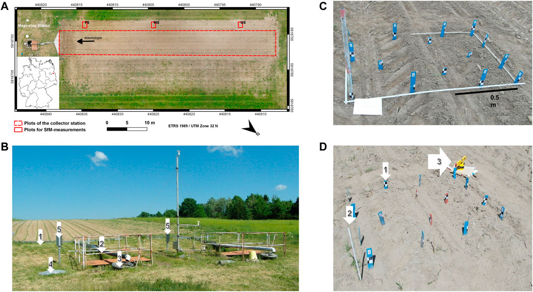
FIGURE 1. (A) Location of the erosion measurement hillsite in Germany (bottom left inlet) and photo image of the hillslope with the collector stations and SfM-plots at the three slope positions: FS (footslope), MS (middle slope), and US (upper slope); (B) Set-up of the erosion measurement station: 1) V-shaped sediment collector, 2) Venturi channel system, 3) sample splitting device, 4) tank, and 5) rain gauge; (C) Experimental set-up for the assessment of soil erosion with SfM at the footslope (FS); (D) Referencing of the GCPs 1) with folding rule 2), and laser level 3).

The automated runoff station at the footslope of the hillslope consists of a funnel-shaped runoff collector (Figures 1B(1)), a system of pipes and channels for distributing runoff water and sediments (Figures 1B(2)), a Coshocton-type sampler for splitting the runoff (Figures 1B(3)) with a subsurface installed automated sample collector with plastic bottles on a turntable, a runoff tank at ground level (Figures 1B(4)), for registration of the total amount of surface runoff, and a Hellmann rain gauge (Figures 1B(5)); the small tower meteorological tower was to measure wind speed, in 20, 50, 100, and 400 cm above the surface.

The plots for structure-from-motion (SfM) photogrammetry were installed on May 3, 2018, at the upper slope (US), middle slope (MS), and footslope (FS) in north-western direction on an identically-tilled area next to the large hillslope-plot (Figure 1A). Since soil erosion rates differ according to slope angle (e.g., Quan et al., 2020) these three plots were chosen for representing the different angles from 3° to 6° present at the hillslope. The potential flow lines at the soil surface of the hillslope runoff experiment determined from a digital elevation model (GlobalMapper 19.0, LiDAR, 2018; resolution: 1.2 cm × 1.2 cm, see Supplementary Appendix SA1) indicated that the SfM plots are not directly connected to the runoff collector at the footslope. The SfM plot size of 1 m length and 1.5 m width was selected such that all surface features (i.e., wheel track, non-compacted region, and 2 rows of corn) were included (Figure 1C) and the area was small enough to achieve mm-resolution due to SfM-processing. The distance between plots at footslope (FS) and MS was 16 m, and between plots at FS and US it was 38 m (Figure 1A). Replicates for the plots could not be identified at this field and were not required since the 3 plots at major hillslope positions could already sufficiently demonstrate the applicability of the SfM-technique and comparison of methods for soil settlement correction. The plots were marked by specially labelled sticks with black-and-white markers for ground control (GC) points (Figure 2). Sticks were driven into the ground down to at least 30 cm depth to ensure that their position was not affected by topsoil porosity changes. Each SfM plot received 15 sticks with GC markers, from which 3 or 4 were placed at the sides and 4 sticks were placed inside of the plot with the GC markers showing in different directions (Figure 1C). The local coordinates of the GC points were determined by using a ruler and a laser level (Einhell Bavaria BLW 400) relative to a reference point at the bottom left corner of each plot (Figures 1D(2)); UTM coordinates were obtained with GPS (Trimble Geo 7X, Handheld GNSS System, accuracy: 0.5–1.0 m) for reference points to determine the position of plots along the hillslope.

FIGURE 2

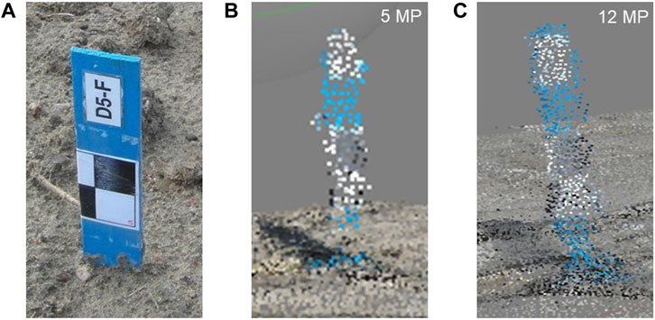
FIGURE 2. (A) Example photo of a ground control point (GCP) at the plot surface and point clouds generated by photos taken with a resolution of (B) 5 MP, and (C) 12 MP.

During the observation period from May 3 to May 16, 2018, two relevant rainfall events occurred on May 3 (5.8 mm) and May 15 (14.4 mm), the latter rain had the highest rain energy (311.5 J m⁻²) and erosivity (EI30) of 6 MJ mm ha⁻¹ h⁻¹ in terms of the maximal 30-min rain intensity (I30). The cumulative rainfall energy E of both events amounted to 406 J m⁻².

The bulk density, ρ_b (kg m⁻³) was determined gravimetrically using 100 cm³ intact soil cores (cylindrical steel cylinders of 5 cm height) by oven drying at 105°C for about 3 days. Samples were determined before the SfM measurements (May 3) and after the heavy rainfall (May 15) from the 1–6 cm soil depth related to the local surface elevation assuming that the value is valid initially after cultivation for most of the topsoil. The top 1 cm of soil could not be sampled without disturbance and was discarded. Since core sampling was destructive, we selected a region outside and downhill of the SfM plots for the sampling. Thus, the plot surface for SfM measurements remained intact and that the potential surface runoff from uphill was not affected by any disturbances of the soil surface. In each field campaign, 6 core samples were taken beneath each SfM plot, of which 3 samples were from the intact cultivated area and 3 soil cores from the area compacted by tractor wheels to capture the variability of soil bulk density related to visible soil structures of the plot (Figure 1C). The number of bulk density samples was limited because of limited soil area in the close vicinity of the SfM-plots that should remain intact for subsequent sampling and runoff observations. Note that each core sampling led to significant disturbance of the intact soil next to the plots. Also, the soil of the larger hillslope measurements should remain intact, thus only a relatively small area for bulk density sampling was available.

The bulk density after the rainfall event on May 15 was alternatively determined from the estimated porosity φ (t) (Linden and van Doren, 1987) as:

$\phi ={\phi }_i-\left({\phi }_i-{\phi }_c\right)\left(1-e^{\left(-aP-bE\right)}\right)(1)$

where φ_i is the initial porosity, φ_c the final porosity of the re-consolidated soil, P [mm] is the amount of rainfall during the event and the cumulative rainfall energy E [J cm⁻²]. The bulk density ρ_b is obtained by

${\rho }_b=\left(1-\phi \right)\ast {\rho }_s(2)$

where ρ_s is the density of the solid particles. The parameters for Eqs. 1, 2 are defined in Table 1. Parameters “a” and “b” in Eq. 1 were fitted manually. The optimization was based on the lowest root-mean-square-error (RMSE) in the mean between the measured and the calculated bulk densities inside and outside the tractor lane in the upper-, middle- and footslope.

TABLE 1

TABLE 1. Original and adapted parameters for Eq. 1: amount of rainfall P, cumulative rainfall energy E, density of solid particles ρ_s, final bulk density ρ_b,c, final porosity φ_c, original and adapted parameters a and b and root-mean-square-error RMSE of the final measured and modelled bulk density; TL: Tractor lane.

SfM-Photogrammetry and Image Processing

Photo images of the plots for SfM-processing were taken on a daily basis with the compact digital camera SAMSUNG WB750 in approximately 1.5 m distance from the plot’s boundaries. The camera has a locked focal length, f, of 4 mm, a maximum aperture of f/3.2 (i.e., a maximum opening width of the objective lens) and a pixel size of 1.49 µm (Samsung, 2011). The DEMs of the soil surface were generated before and after two rainfall events. Each plot was photographed 30–50-times from different perspectives to ensure a spatial overlapping of the images of at least 60% as suggested previously (Westoby et al., 2012; Kaiser et al., 2015). There was no need to adjust the camera to similar perspectives or heights for subsequent photo-sessions at different days, since the camera positions were automatically determined during the image processing, and ground control points (GCP) ensured the georeferencing of the 3D-models. This was one of the major advantages of the SfM-photogrammetry in comparison to, e.g., laser scanning. A sensor size of 5 Mega Pixel (MP) (2592 × 1944 pixels) was used for the images during the initial period (May 2 to May 14) and a size of 12 MP (4096 × 3072 pixels) for the images taken until May 16. The 12 MP images were downscaled to a pixel sensor size of 5 MP before processing with Adobe Photoshop Elements (Adobe Systems, 2018 Adobe Photoshop Elements Version: 15.0 (20160905. m.97630) x64, operation system: Windows 8.1 64-Bit,Version: 8.1). The point cloud obtained with VisualSfM (Figure 2) appeared to have more evenly distributed points, as compared to a point cloud generated from original 5 MP images. This advantage of downscaling the pictures was found throughout the experiemental period, such that images were only taken in 12 MP resolution at the end of the observation period.

The image processing was carried out with the freely available software VisualSfM (Wu, 2011); the workflow (Figure 3) depicts the applied software for each of the subsequent steps, starting with the image alignment and the reconstruction of the sparse and the dense point clouds that were combined to 3D point clouds. The sparse point cloud contains all points that are found in three or more pictures (Westoby et al., 2012). The dense point cloud contains additional points that are reconstructed by the application of the CMVS- and PMVS2-algorithms. In VisualSfM, the Scale Invariant Feature Transform (SIFT) was used to identify common points and structures in the images independent of their size, illumination, and rotation. The Bundle Block Adjustment (BBA) carried out non-linear 3D spatial optimization of camera position related to GC points (Figure 1D) to find the common structures on images for generation of a condensed point cloud. The Clustering View for Multi-view Stereo (CMVS) routine divided data obtained with BBA-algorithm in smaller easier to handle point cloud clusters as a first step to aggregate the combined point cloud. Finally, the Patch-based Multi-view Stereo (PMVS2) routine was applied to independently reconstruct the 3D-spatial data clusters obtained with the CMVS as the second step in point cloud aggregation.

FIGURE 3

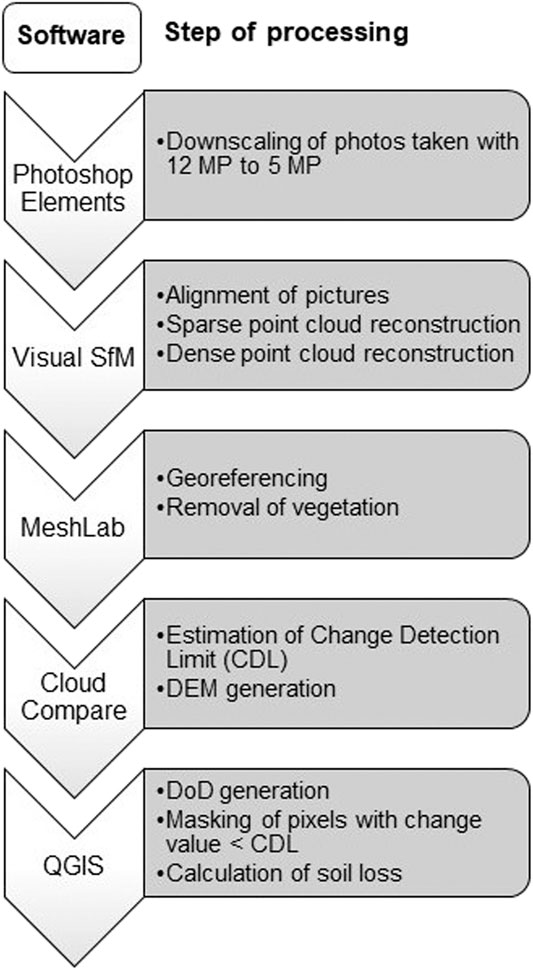
FIGURE 3. Workflow of SfM-photogrammetry data processing.

After the Visual SfM step (Figure 3), georeferencing of the 3D point clouds was carried out by assigning the measured local coordinates to 4 of the reconstructed GC points (Figure 1D) using MeshLab software (Cignoni et al., 2008; Cignoni, 2016). All points resulting from above-ground vegetation (i.e., maize plants) were manually removed in the May 16th surface models (i.e., end of the observation period). The Level of Detection (LoD) was then estimated using CloudCompare software (Cloud Compare, 2020 CloudCompare V2, EDF R&D/TELECOM ParisTech (ENST-TSI), Paris 2016) before exporting the DEMs derived from the point clouds to QGIS software (QGIS Development Team, 2018). The DEM generated from images after a rain event was subtracted from that derived from images before the event in QGIS to create a map of the pixel-based changes in soil surface micro-topography (for images of the workflow see Supplementary Appendix SA4). These DEMs of temporal Difference (DoD) were corrected for the uncertainty in the determination of the re-location of GC points by assigning a value of zero to all pixel values smaller than the LoD. Thus, we assumed that uncertainties caused by small differences in referencing the DEMs of two times were negligible. The plot-average changes in soil surface elevation, ${\overline{\Delta z}}^{\Delta t}$ between two times, $\Delta t=t_2-t_1$ were obtained from the sum of DoD pixel values, $\Delta z_i$ divided by the number of pixels, N_p = 1, … , i, as:

${\overline{\Delta z}}^{\Delta t}=\frac{1}{Np}{\displaystyle \sum _{i=1}^{Np}\Delta z_i}.(3)$

The LoD is defined as the smallest value of change in soil elevation that can actually be detected with SfM without being considered as noise. For the determination of the LoD only those GC points were deployed that were not used for georeferencing. For the LoD different definitions exist in the literature (e.g., Brasington et al., 2003). Here, the LoD between two measurements, $\Delta t$, is calculated from the differences of the x-, y-, z-coordinates (isotropic) in all directions as

$Lo{D}^{\Delta t}=\sqrt{\frac{1}{n\ast k}{\displaystyle \sum _{i=1}^n{\displaystyle \sum _{j=1}^k\left[{\left(X_{P_{i,j}}^{t2}-X_{P_{i,j}}^{t1}\right)}^2\right]}}}(4)$

where X denotes the k = 3 coordinates of the n = 4 GC points (P_i,j) at times t₁ and t₂.

The component describing surface elevation changes due to consolidation and natural compaction (e.g., by rain impact) was considered by the mean surface elevation changes, ${\overline{\Delta z}}_{cs}^{\Delta t}$ (subscript cs denotes “compacted soil”), obtained from the original $\left({\overline{z}}_{ts}^{ t1}\right)$ mean elevation (subscript ts means “tilled soil”) and the soil bulk density relations before $\left({\rho }_b^{t1}\right)$ and after the rain event $\left({\rho }_b^{t2}\right)$ (Hänsel et al., 2016) as:

${\overline{z}}_{cs}^{t2}=\left({\rho }_b^{t1}/{\rho }_b^{t2}\right)\ast {\overline{z}}_{ts}^{t1}(\mathrm{5a})$

where the thickness of tilled soil before the rain at t₁ was first assumed to correspond with the height of the soil core of 5 cm. The value of ${\overline{z}}_{cs}^{t2}$ (here in mm) depends on the thickness of the cultivated soil region, considered to be affected by consolidation; here we compare the effect of a thickness of 5 cm with that of when assuming a value of ${\overline{z}}_{ts}^{t1}$ of 10 cm. Other values were not considered because major elevation changes due to consolidation during single rain events are expected to occur within the uppermost 0–10 cm layer of the topsoil (Rousseva et al., 1988). The two different thickness values were assumed as possible range, since we did not know, whether the bulk density changes occurred in the upper 5 cm of the soil or reached down to 10 cm. Different consolidation was measured outside (2/3 of the plot) and inside the tractor lane (1/3 of the plot). This was accounted for by weighing the soil surface elevation change in the different parts of the plots as:

${\overline{z}}_{cs}^{t2}=\left({\rho }_{b,i}^{t1}/{\rho }_{b,i}^{t2}\right)\ast {\overline{z}}_{ts}^{t1}\ast \frac{1}{3}+ \left({\rho }_{b,o}^{t1}/{\rho }_{b,o}^{t2}\right)\ast {\overline{z}}_{ts}^{t1}\ast \frac{2}{3}(\mathrm{5b})$

The subscripts “i” and “o” denote “inside” and “outside” the tractor lane, respectively.

The plot-related mean settlement-induced component of the reduction in soil surface elevation, ${\overline{\Delta z}}_{cs}^{\Delta t}=\left({\overline{z}}_{cs}^{t2}-{\overline{z}}_{ts}^{t1}\right)$, was subtracted from the mean changes in surface elevation obtained from either the DoD maps between the two times, ${\overline{\Delta z}}^{\Delta t}$, Eq. 3, to yield a corrected mean value of surface elevation changes as:

${\overline{\Delta z}}_{cor}^{\Delta t}={\overline{\Delta z}}^{\Delta t}+{\overline{\Delta z}}_{cs}^{\Delta t}(6)$

where subscript cor denotes “corrected”.

The fraction of the area of which the soil surface elevation increased, decreased or remained unchanged was calculated for the main soil surface structural areas of the plots. The surface structures inside the tractor lane (in TL), outside the tractor lane (out TL), and the seed row (SR) were defined and manually distinguished according to the visible structures in the DoDs. The DoDs of each plot were reduced to the individual soil surface structure and pixels were classified according to increase (+), decrease (−) and no change (0) in soil height and the number of pixels in each class was summed up. The area fraction of each class of soil surface structural feature was obtained (c.f., Eq. 3) from the sum of pixels divided by the total number of pixels.

Potential Errors in Data Acquisition and Processing

Throughout the process of soil loss determination by SfM several errors accumulate: 1) GC points were manually levelled, 2) the generation of the dense point clouds in Visual SfM depends on the image quality and leads in case of low quality images to a lesser point density causing errors when creating surface models 3) georeferencing errors, and 4) errors in soil loss calculation from soil elevation changes due to natural consolidation.

Here, the levelling the GC points with the laser level with an accuracy of ±1 mm. The standard deviation of georeferencing the point clouds in MeshLab and the calculation of the Level of Detection (LoD) in CloudCompare amounts to 0.7 mm. For the bulk density measurements used for the correction of soil settlement, a mean standard deviation for all plots of 70 kg m⁻³ was obtained. This value resulted in an error of 0.5 mm if a 5 cm topsoil layer ${\overline{z}}_{ts}^{t1}$ and of 1.1 mm if a 10 cm topsoil layer ${\overline{z}}_{ts}^{t1}$ is assumed (Eq. 5a). Thus, these errors add to a maximal value of either 2.2–2.8 mm if all sources of possible inaccuracies in data acquisition and processing are considered.

Calculation of Soil Surface Roughness

Soil surface roughness, as an important input for soil erosion models (e.g., Kaiser et al., 2015), was calculated in QGIS by employing the roughness algorithm derived from the GDAL DEM utility (QGIS Development Team 2014). This algorithm derives the roughness from the Terrain Ruggedness Index (TRI) according to Wilson et al. (2007) by averaging the absolute values of the differences in height between a pixel and its 8 neighbors. This algorithm was used because it provided a convenient and quick possibility to characterize morphologic soil surface changes within the plots. It was the only algorithm currently implemented in QGIS to determine soil roughness. In order to obtain an average roughness of the whole plot, the values of all pixels per plot were averaged.

Results

Soil Bulk Density

Soil bulk density was initially higher in the tractor lanes (1,430–1,480 kg m⁻³) than in the soil regions between tractor lanes with 1,180–1,270 kg m⁻³ (Table 2, for statistical analyses see Supplementary Appendix SA2). Measured soil bulk density increased within the 20 days in most plots, except for the tractor lane regions on the middle and upper slopes; however, this effect of a decrease in soil bulk density was smaller than the standard deviation and negligible. The soil outside of the tractor lanes was generally more compacted at the second date indicated by a density increase of about 80–100 kg m⁻³ as compared to the first date and the soil within tractor lanes. On the plot at the footslope position, soil regions in and outside the tractor lanes were similarly more compacted as indicated by a density increase of 70–80 kg m⁻³. According to statistical analysis the bulk density differences between inside and outside the tractor lane were not significant, except for the middle and upper slope on May 2, 2018 (Supplementary Appendix SA2). The predicted bulk density for the May 22 was similar to the measured bulk density outside the tractor lane. However, modelling showed a stronger increase in soil bulk density inside the tractor lane than the measurements suggested (Table 2).

TABLE 2

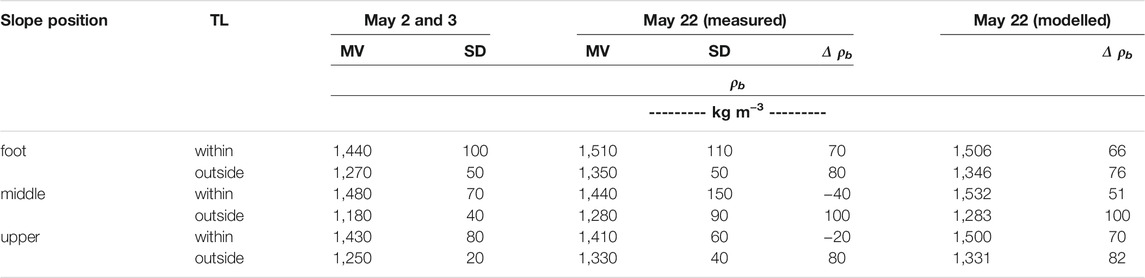
TABLE 2. Surface soil (1–6 cm depth) bulk density, ρ_b (kg m⁻³), for the SfM-plots at the three slope positions determined from samples taken inside and outside of the wheel track of a tractor lane (TL) on May 2 and 3 and on May 22, and differences between the two times, Δ(for statistical significant differences see boxplots in Supplementary Appendix SA2); mean values (MV) and standard deviation (SD) from 3 replicates. TL, Tractor lane.

SfM-Measurements of Surface Structural Changes and Soil Loss

The final DoD-maps (Figure 4) show spatially-distributed patterns of increasing (green) and decreasing (red) soil surface elevations. The tractor lanes and the seed rows could be identified more clearly in the individual DEMs provided in the Appendix (Supplementary Appendix SA5). For the upper slope position, only relatively small changes in soil surface topography are noticed during the first 2 days after the installation of the plots (Figure 4A, top). Settlement of the soil can be observed more in the less compacted right part of the plot as compared to the more compacted seed rows and tractor lanes. After 12 days (Figure 4A, centre), the settling of the soil was more pronounced (i.e., more decreasing surface elevations) also in the plot region of the initially more compacted soil. Note that the first leaves of the maize plants could be identified as spots of larger elevation increase along the seed row in the middle of the plot. After the heavy rainfall event on May 15, the increased red spots in the lowest DoD map (Figure 4A, bottom) indicated a larger decrease in soil surface elevation esp. in the less and more compacted regions of the plot, where more than 80% of the area was subject to soil height loss (Figure 5).

FIGURE 4

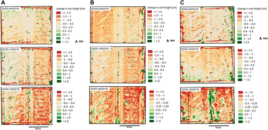
FIGURE 4. Maps of changes in soil surface elevation (micro-topography) calculated from the SfM-derived DEM’s of two dates (i.e., DoD) at the plots of (A) the upper-, (B) the middle-, and (C) the footslope position during the period between May 2 and May 16; see Supplementary Appendix SA5 for DEMs.

FIGURE 5

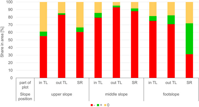
FIGURE 5. Share in area that increased (+), decreased (−) or did not change (0) in the individual soil surface structural sections tractor lane (in TL), outside tractor lane (out TL) and seed row (SR) at the upper, middle and footslope from May 02 to May 16.

For the plots at the middle- (Figure 4B) and the footslope (Figure 4C) positions, the changes in soil surface topography are relatively similar during the first period between May 2, 4, and 14 (upper and central rows of the maps in Figure 4). An exception is the plot at the middle slope: the decrease in surface elevation was stronger in the more compacted tractor lane than in the looser region of the plot (Figure 4B, top). Twelve days later, the situation has changed completely: now the loose area shows higher settlement than the tractor lane (90% of the area outside the tractor lane was subject to soil height loss, Figure 5). This might be attributed to the different values in the level of detection, LoD, assigned to the DoDs. Changes in soil surface elevation could be masked by a higher limit used as LoD. On May 16, due to rainfall the soil surface elevation is more strongly decreasing (red spots) than increasing (green spots) especially for the plot at the middle slope (Figure 4B, bottom). Deposition of soil can be observed at the middle slope plot especially at the lower end of the seed row and in the imprints of the tyres. For the plot at the footslope position, the regions with an increase in surface elevation or deposition are largest and oriented along the seed row along the central part (Figure 4C, bottom and Figure 5); for this plot at the footslope, a gradient in surface elevation changes was observed ranging from decreasing elevations (erosion) in the upper to increasing elevations (deposition) in the footslope regions. Red and green spots next to each other, especially for plots at the middle and the bottom slope position (Figures 4B,C, maps at the bottom), indicate a flattening of the soil surface topography due to deposition, of soil particles that were detached at the local peaks for example, within the wheel tire marks.

Between May 02 and 16, the plot at the upper slope position experienced the smallest changes in mean surface elevation. This means that here a larger area of the plot remained at the same surface elevation than at the middle slope and footslope (Figure 5). As observed qualitatively the middle slope had the highest surface area fraction with soil height loss in all soil surface structural regions (>80%). For the footslope, the seed row experienced the most pronounced increase in soil height, since 40% of the seed row area fraction increased in soil height (Figure 5).

The plot-scale averages of the changes in soil surface elevation obtained from the DoD-maps between May 14 and May 16 were all larger as compared to the hillslope-related calculated soil loss of the sediment yield of the collector station (Table 3). The plot-scale mean elevation changes were all negative except for the plot at footslope position, if considering no soil consolidation and consolidation related to 5 cm topsoil (Figure 6). When consolidation was related to 10 cm topsoil, all plots (upper-, middle- and footslope) showed increase in soil surface elevation, except when no consolidation was accounted for (Figure 6).

TABLE 3

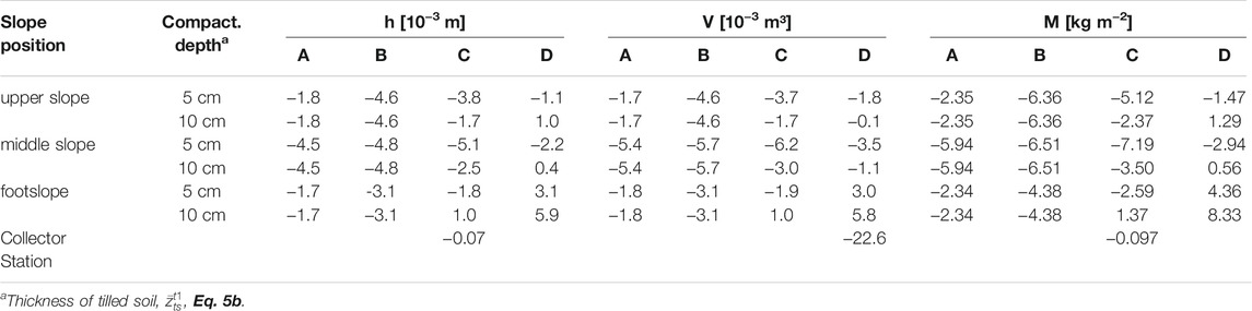
TABLE 3. Weighted changes in average soil surface elevation (h), volume (V), and mass (M) at the SfM-plots along the experimental slope between May 2 and A: May 4, B: May 14, and C: May 16; D indicates changes in surface elevation and mass between May 14 and 16 after correction for soil settlement; mass, M, collected at the hillslope erosion station between May 2 and 16 (C) was used to calculate a slope-averaged value of the change in surface elevation (h) over the total hillslope.

FIGURE 6

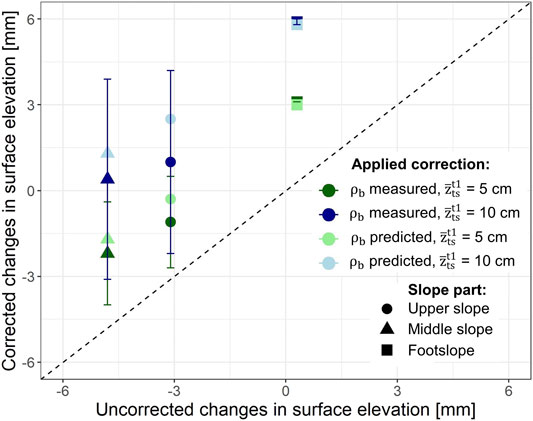
FIGURE 6. Uncorrected vs. corrected soil elevation changes [mm] between May 14 and May 16 in the upper slope, middle slope, footslope. The soil height elevation changes were corrected for consolidation by the measured final bulk density ${\rho }_b$ assuming a thickness of the tilled soil, ${\overline{z}}_{ts}^{t1}$, of 5 and 10 cm and corrected for consolidation by the predicted final bulk density ${\rho }_b$ assuming a thickness of the tilled soil, ${\overline{z}}_{ts}^{t1}$, of 5 and 10 cm.

The plot-scale averages of the changes in soil surface elevation depict values between −6 and −2 mm that are dependent on the slope (Figure 7A). One exception is the positive value found for the plot at the bottom slope position indicating predominately deposition during the rain event. The plot at the upper slope (Figure 7A) with the smallest inclination (6%) showed smallest elevation changes (−1.8 mm) but relatively large changes due to consolidation of approx. -5 mm (Table 3). The plot at the middle slope with 9% inclination experiences the most pronounced surface changes (−2.2 mm) and consolidation (up to −5.4 mm). Although the inclination was largest at the plot at the footslope (11%), only relatively small changes (−1.7 to −3.1 mm) in the mean surface elevation were observed before and deposition (+3 mm) was observed after the rainfall event on May 15 (Table 3). The plot at the middle slope shows the highest losses in surface elevation in contrast to the plots at the upper- and footslope, which corresponded with the loss in soil volume and soil mass (Table 3).

FIGURE 7

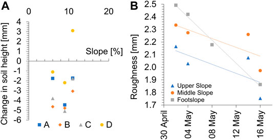
FIGURE 7. (A) Corrected changes in soil elevation assuming a thickness of the tilled soil, ${\overline{z}}_{ts}^{t1}$, of 5 cm since May 2 dependent on the slope at different times: A–May 4; B–May 14; C–May 16; D–temporal change in soil elevation between May 14 and May 16; (B) Soil roughness change at the upper-, middle- and footslope between May 2 and May 16 (The DEM of the footslope was created at May 8 instead of May 14 since the image quality of the pictures taken on May 14 did not proof to be sufficient to generate a DEM).

The average soil roughness in terms of the Terrain Ruggedness Index (TRI) decreased at all plots from May 2 till May 16 (Figure 7B). The plot at the footslope had the highest initial soil roughness with 2.5 mm, whereas the upper slope had the smallest initial soil roughness (2.2 mm). Throughout the observation period, the footslope position showed the strongest decrease of TRI-values from 2.5 to 1.9 mm, which corresponds to the deposition and levelling of the soil surface that was observed for the plot surface at the footslope position. At middle and upper slope positions, TRI values decreased only by approximately 0.4 mm from 2.3 to 2.0 mm and 2.1 to 1.7 mm. The soil roughness of the soil surface at the footslope position most gradually decreased (Figure 7B), while at the middle and upper slopes, the surface roughness decreased initially more strongly from May 2 till May 4, remained at the same level till May 15, and decreased again after the rainfall on May 15.

Comparison of Methods for Soil Settlement Correction and Comparison to Slope

The subplots for soil erosion assessment with SfM, installed at the upper, middle, and footslope position of the hillslope differed with respect to slope inclination. After correcting the mean soil surface elevation changes of these plots by using predicted bulk density changes, the elevation changes were generally smaller as compared to the changes obtained by using measured bulk density for the correction (Table 4). Both, measurements and predictions, resulted in an overall reduction in original mean surface elevation of the tilled soil $\left({\overline{z}}_{ts}^{t1}\right)$ for plots at the upper and the middle slopes. However, an increase in soil surface elevation was found for the plot at footslope position when the settlement correction was related to a 5 cm soil layer. When bulk density changes were assumed to affect a soil layer of 10 cm thickness, a net deposition was obtained for plots at the upper, middle, and footslope positions. Here, the predictions of the soil settlement correction led to larger values of the surface elevation changes as compared to the measurements (Table 4).

TABLE 4

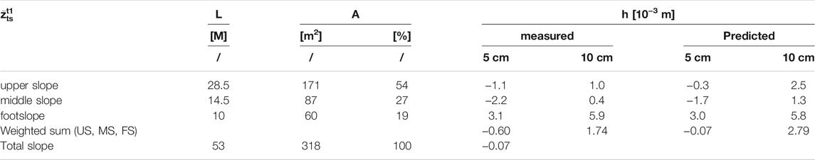
TABLE 4. Slope length (L) and area (A) of the different slope sections (in m² and % of the total slope) of the total slope together with weighted changes in average soil surface elevation (h) (according the share of each slope part of in the total slope) corrected by the measured and predicted soil bulk density (Eq. 1) at the SfM-plots along the experimental slope between May 14 and 16 after correction for soil settlement; ${\overline{z}}_{ts}^{t1}$ denotes the applied correction value for the compaction depth of 5 and 10 cm; the weighted sum describes the average loss in soil elevation derived from the SfM-plots extrapolated to the total slope and weighted by the different area sizes.

Although the soil loss observed by SfM at the smaller plots cannot quantitatively be compared to soil loss by surface runoff and erosion at larger slopes (Parsons, 2019, see discussion 4.4), an extrapolation may be useful to check the plausibility range of the SfM data and evaluate ranges and relative soil masses quantified with the SfM method. Still, for comparing subplot information with those of the hillslope, the soil mass changes determined at the SfM-plots need to be weighted, here according to the upper-, middle-, and footslope area fractions (Table 4). Note that the typical relations between slope lengths and relative sizes of slope sub-divisional areas (Jha et al., 2015) was modified by increasing the length of the footslope sub-division from 3 to 10 m and proportionally reducing the length of the middle slope to account for the observation of deposition along this 10 m slope region (Supplementary Appendix SA3). The soil loss measured in the collector station was in the range of SfM-measurements corrected by using the predicted bulk density changes according to Linden and van Doren (1987) when assuming a topsoil height of 5 cm. With the correction based on measured bulk density values related to a 5 cm thick topsoil, the soil loss extrapolated by the SfM-technique for the total slope was 8- to 9-times that observed at the hillslope station (Table 4). The correction of the soil settlement applied to a topsoil height of 10 cm led to an increase in soil surface elevation after the erosion event for all plots (Figure 6 and Table 4).

Discussion

Soil Loss and Surface Structural Changes Obtained by SfM

Soil surface structural changes due to raindrop impact could be quantified with the SfM-technique at the three hillslope positions. The plot located near the footslope received more sediments than were eroded (Table 3) because in these regions, any surface runoff coming from upper slope regions is saturated with sediments and cannot take up more soil particles (Schmidt, 1996). For plots at middle and upper slope positions, surface runoff only locally affected the surface roughness (Figure 7B, Supplementary Appendix SA5) and probably generated not sufficient kinetic energy for initiating larger-scale erosion under the present conditions and slope angles. The observed internal distribution of the soil within one SfM-plot with similar slope angle (10%) was also found in the study by Quan et al. (2020) with soil elevation increase at the lower end of the plot. Kaiser et al. (2018) and Hänsel et al. (2016) reported similar local redistribution of soil from the exposed higher elevated plot regions into the depressions and lower elevated regions.

Between May 02 and 16, the plots show a decrease in soil surface elevation in all surface structural units (Figure 5). In the plot at upper slope position, larger area fractions remained unaffected from these changes than in the plots at middle and footslope positions. Since soil erosion is unlikely to occur so far upslope due to insufficient kinetic energy of the runoff (Schmidt, 1996) and according to visual inspection, soil consolidation must have been the main reason for soil surface elevation reduction. Note that the area fraction for which elevation changes were observed with SfM for the soil surface structural regions is not directly related to the amount of soil erosion in the plot. Relatively small areas of the plot with relatively large elevation changes could have affected the overall plot scale mass changes.

The decline in soil surface roughness (Figure 7B) could be attributed to the collapse of soil aggregates. Mechanisms for aggregate breakdown have been attributed to contractive forces of water in menisci between soil particles (Hartge et al., 2014), the decrease in structural stability of soil aggregates during wetting (Bergsma und Valenzuela, 1981), the destruction of soil aggregates by rain drop impact (Bolt and Koenigs, 1972) and the subsequent transport of smaller particles into larger pores (Schmidt, 1988). The soil surface maps at the footslope position with the strongest decrease in soil roughness supported the observation that soil particles were deposited in the local depressions leading to a levelling of the profile (Figures 4, 5, 7B). The small effect of slope inclination on soil surface dynamics was probably related to relatively high infiltration rates at the upper and middle slope positions, and the focused surface runoff on cultivation-induced features such as wheel tracks and plant rows (Supplementary Appendix SA3).

Comparison and Limitations of Techniques for Soil Consolidation Estimation

Soil loss estimated by SfM-photogrammetry was smaller when soil consolidation was accounted for either by bulk density measurements or predictions (Eq. 1) according to Linden and van Doren (1987) (Table 4). This seems more plausible because the overall soil loss of the total slope was significantly smaller than those derived from plot-scale data (Table 3). Soil consolidation needs to be considered as an important source for soil elevation decrease of a freshly cultivated soil in temperate climate zones (Schmidt, 1988).

When comparing the measurement with the prediction of soil settlement correction, similar trends for the overall change in soil height of the plots can be found: A decrease in soil height for the upper and middle slopes and increase (i.e., net deposition) for the footslope position (Table 4). The prediction method has the advantage that no elaborate bulk density measurements are needed after each precipitation event. Measurement errors of the soil bulk density can lead to larger errors, so a lot of soil samples need to bet taken and larger soil areas need to be disturbed for the sampling. In case of the bulk density prediction, however, site-specific characteristics cannot directly be included in the analysis. Additionally, data of bulk density changes as determined here by core sampling, cannot clearly distinguish between natural soil settlement and erosion or deposition (e.g., Knapen et al., 2008). Both processes might lead to a change in bulk density in addition to natural consolidation due to raindrop impact. An alternative approach in this case would be to determine the bulk density changes in a levelled area (i.e., control plot) that is not subject to soil erosion but only to natural soil consolidation via rainfall. However, this plot would have to be located in the vicinity to the sloped plot, to ensure comparable raindrop impact and soil conditions. To install such a control plot in the field, might be challenging; and could be only tested under simulated rainfall and in the laboratory (e.g., Kaiser et al., 2018). The settlement prediction considers bulk density changes only due to raindrop impact for levelled plots and thus predicts final bulk densities without the impact. The advantage of the prediction over the direct measurements is that the model could be calibrated by fitting parameters “a” and “b” to site-specific bulk density changes observed when erosion impact could be excluded.

Limitations Caused by SfM-Data Processing

Besides deviations caused by conditions in the field, uncertainties might occur also throughout the SfM-processing due to low precision in georeferencing of the 3D point clouds in MeshLab. Because of limited computational power, dense point clouds were not generated for every single part of the plots. In most cases, the centre of the GCPs was not exactly represented by a single point but was rather located in between two points. Consequently, throughout the georeferencing process only one of the points located a certain distance away from the actual GCP centre could be chosen for georeferencing leading to a deviation from the real coordinates. The described georeferencing error has been accounted for by considering a detection level, LoD (Figure 7, legends).

Between the points of the 3D point cloud, an interpolation was carried out in areas with a low point density during DEM generation in CloudCompare. This is the case especially in the regions close to the plot boundaries, where the coverage with images was lower than in the plot centre. For every time step, VisualSfM produced different point clouds depending on the photo images. This was also the case, when two 3D models of the same object were generated from a different set of pictures. Hence, for both 3D models, different point clouds existed as a template for the DEM generation so that interpolation between the points was different leading to differences in the DEMs of the same object. This interpolation error increased with the complexity of an object’s surface. Since soil surfaces were rather heterogeneous, this error was probably important. A possible solution could be to use pictures with a higher image resolution (Figure 2; i.e., from 5 to 12 MP). Unfortunately, VisualSfM software was unable to process such highly resolved data. By the use of downscaled pictures from 12 MP to 5 MP in Photoshop Elements, the point cloud density was not increased but the points were more evenly distributed throughout the point cloud. Other software such as PhotoScan (Agisoft, 2018) would be better able to handle a variable amount of data points (Jiang et al., 2020). However, this software was not available and required more computational power.

Challenges of small-scale erosion quantification by SfM and future needs.

The SfM-photogrammetry proved to be a useful tool to observe small scale soil surface micro-topography and structural changes at three plots or subplots along a hillslope. The advantage of our case study carried out in combination with the hillslope erosion experiment was that the same agricultural management was carried out uniformly over the whole field and that the basic conditions, soil, crop, tillage, and weather information could be directly used and compared with the complete hillslope. However, the soil loss found at the SfM-plots could not be related to that measured at the hillslope collector station for several reasons: For a start, the origin of the sediments collected at the footslope is uncertain, and according to the surface flow lines, sediments may have also passed the funneled collector (c.f. Supplementary Appendix SA1). It is not clear, where the sediment in the collector station might have come from. Travel distances of particles is finite and small (Parsons et al., 2010), thus the small plots can only estimate local redistribution. Also, the suggested approach to relate soil surface elevation changes of a smaller slope to the average soil surface elevation changes of a larger slope (Table 4) is dependent on the empirically adjusted slope length among other factors. Thus, this approach is site specific and cannot be transferred to other areas. Similar comparisons of smaller plots to larger slopes (Chaplot and Poesen, 2012) gave considerably higher sediment delivery rates from 1 m² plots as compared to hillslope-scale (899 versus 4.3 g m⁻² y⁻¹). These authors attributed this discrepancy to splash erosion being the dominant sediment detachment and transport mechanism at hillslopes. Martinez et al. (2017) also found lower sediment yields at larger plots (27 m²) as compared to smaller plots (0.7 m²). In contrast, Boix-Fayos et al. (2007) found higher sediment concentrations at larger plots (30 m²) than in 1 m²-sized plots.

Thus, the observed discrepancies between the different soil loss estimation techniques in this study can be attributed to the smaller size of the plots used for the SfM-measurements (1.5 m²) in contrast to the collector station that accumulates the eroded sediment from a 318 m² hillslope. The SfM-plots reveal the local deposition and erosion processes and do not allow estimating processes between plots (Parsons et al., 2010). Any comparison would improve, if DoD maps of the hillslope were generated provided the SfM-technique could be applied to the total area. Unfortunately, the resolution of the DoDs for a larger area would still be too coarse, the identification of effects of rain events on surface structure dynamics is limited (Kaiser et al., 2018). On the other hand, one could separate larger hillslopes into smaller areas (1–3 m²) that are each observed in detail with SfM and finally merged into a large DoD maps.

The SfM measurements basically provide quantitative and spatially-distributed information on the surface topography; it is not possible to distinguish between deposition of soil from uphill and erosion of soil that left the plot and the settlement. Furthermore, the change in the surface micro-topography includes the decline in surface roughness after rain. This may be considered as a kind of local erosion and deposition, which makes it difficult to separate between the deposition from uphill and local processes. The separation between input and output from changes in mean surface elevation requires additional assumptions that could be based on observations at the neighboring hillslope as follows:

Upper slope position: Based on observations it may be assumed that here the deposition from above was negligibly small such that the changes in surface elevation can be explained by runoff soil loss and by settlement.

The soil surface at the middle slope is in a through-flux position and has both deposition from above and soil loss towards downhill positions. Soil settlement could be the main unknown when assuming that lateral inputs equal outputs of soil mass. At the footslope position, there is clearly more deposition than erosion such it is assumed that the surface elevation changes account for net accumulation and some settlement.

Note that the observations do not allow to exactly quantify the rates of the different components of the soil mass changes but we can provide information on potentially relevant limits by making estimates when assuming minimal and maximal ranges limits from the comparison with the data obtained at the complete hillslope.

Conclusion

The application of SfM-photogrammetry on a bare soil allowed quantifying differences in soil surface elevation and structure dynamics due to the impact of rainfall, erosion, and consolidation on soils freshly sowed with Maize. Maps of local or micro-topographic changes were generated for plots at three hillslope positions.

The results of testing different soil consolidation rates in form of soil bulk density changes in topsoil layers indicated that it would be necessary to better account for the structure dynamics in the entire topsoil volume when trying to estimate the elevation changes caused by natural consolidation. The results of the comparisons between data and regression approach suggest that the relatively simple regression after calibration can be useful to correct soil surface elevation changes induced by rain for natural soil settlement.

The results of the soil mass balancing of the plots from the difference between SfM surface elevation maps before and after a rain event revealed also uncertainties that resulted from georeferencing and computation limits of the used software.

The SfM technique designed for the non-destructive and repeated monitoring of soil surface structural dynamics under field conditions, provided valuable information on soil structure parameters such as surface roughness. Improvements could be achieved by using higher resolution images and expanding the SfM-application to the hillslope.

The results suggest that the use of widely available cameras and application of freely available software for processing photos and DEMs is possible. This may stimulate the application and monitoring of erosion-affected soil surface changes in many arable soil landscapes and regions with limited accessibility. Further improvements of the standardized application, the accuracy, and the calibration of empirical bulk density models are still necessary.

Data Availability Statement

The original contributions presented in the study are included in the article/Supplementary Material, further inquiries can be directed to the corresponding author.

Author Contributions

AE: Conceptualization; Data curation; Formal analysis; Investigation; Methodology; Software; Validation; Visualization; Writing-original draft; Writing-review and editing. HG: Conceptualization; Methodology; Supervision; Validation; Writing-review and editing. DD: Resources; Methodology; Supervision

Funding

The research was funded by the Leibniz Centre for Agricultural Landscape Research (ZALF), which is a research institution of the Leibniz Association in the legal form of a non-profit registered association. ZALF is financed in equal parts by the Federal Ministry of Food and Agriculture (BMEL) and the Ministry for Science, Research and Culture of the State of Brandenburg (MWFK).

Conflict of Interest

The authors declare that the research was conducted in the absence of any commercial or financial relationships that could be construed as a potential conflict of interest.

Publisher’s Note

All claims expressed in this article are solely those of the authors and do not necessarily represent those of their affiliated organizations, or those of the publisher, the editors and the reviewers. Any product that may be evaluated in this article, or claim that may be made by its manufacturer, is not guaranteed or endorsed by the publisher.

Acknowledgments

We thank Anette Eltner (Technical University Dresden) and Phoebe Hänsel (Technical University Bergakademie Freiberg) for support in handling or application of the SfM-technique and software and Lidia Völker (ZALF Müncheberg) for plotting surface flow maps of the hillslope.

Supplementary Material

The Supplementary Material for this article can be found online at: https://www.frontiersin.org/articles/10.3389/fenvs.2021.737702/full#supplementary-material

References

Adobe Systems (2018). Adobe Photoshop Elements. Available at: https://www.adobe.com/de/products/photoshop-elements.html 10 (Access date: 19, 2018).

Google Scholar

Agisoft (2018). PhotoScan. Available at: https://www.agisoft.com/03 Access date: 21, 2020).

Google Scholar

Ahuja, L. R., Ma, L., and Timlin, D. J. (2006). Trans-Disciplinary Soil Physics Research Critical to Synthesis and Modeling of Agricultural Systems. Soil Sci. Soc. Am. J. 70 (2), 311–326. doi:10.2136/sssaj2005.0207

CrossRef Full Text | Google Scholar

Ahuja, L. R., Rojas, K. W., Hanson, J. D., Shaffer, M. D., and Ma, L. (2000). Root Zone Water Quality Model: Modeling Management Effects on Water Quality and Crop Production. Highland Ranch, CO: Water Resources Pub., LLC.

Google Scholar

Bendig, J., Bolten, A., and Bareth, G. (2013). Monitoring des Pflanzenwachstums mit Hilfe multitemporaler und hoch auflösender Oberflächenmodelle von Getreidebeständen auf Basis von Bildern aus UAV-Befliegungen. pfg 2013, 551–562. Available at: https://kups.ub.uni-koeln.de/20608/. doi:10.1127/1432-8364/2013/0200

CrossRef Full Text | Google Scholar

Bergsma, E., and Valenzuela, C. R. (1981). Drop Testing Aggregate Stability of Some Soils Near Merida, Spain. Earth Surf. Process. Landforms 6, 309–318. doi:10.1002/esp.3290060310

CrossRef Full Text | Google Scholar

Boardman, J. (2006). Soil Erosion Science: Reflections on the Limitations of Current Approaches. CATENA 68 (2-3), 73–86. doi:10.1016/j.catena.2006.03.007

CrossRef Full Text | Google Scholar

Boix-Fayos, C., Martínez-Mena, M., Arnau-Rosalén, E., Calvo-Cases, A., Castillo, V., and Albaladejo, J. (2006). Measuring Soil Erosion by Field Plots: Understanding the Sources of Variation. Earth-Science Rev. 78 (3-4), 267–285. doi:10.1016/j.earscirev.2006.05.005

CrossRef Full Text | Google Scholar

Boix-Fayos, C., Martínez-Mena, M., Calvo-Cases, A., Arnau-Rosalén, E., Albaladejo, J., and Castillo, V. (2007). Causes and Underlying Processes of Measurement Variability in Field Erosion Plots in Mediterranean Conditions. Earth Surf. Process. Landforms 32 (1), 85–101. doi:10.1002/esp.1382

CrossRef Full Text | Google Scholar

Bolt, G. H., and Koenigs, F. F. (1972). Physical and Chemical Aspects of the Stability of Soil Aggregates. Ghent Rijksfac Landbouwetensch Meded 29, 955–973.

Google Scholar

Borrelli, P., Robinson, D. A., Fleischer, L. R., Lugato, E., Ballabio, C., Alewell, C., et al. (2013). An Assessment of the Global Impact of 21st century Land Use Change on Soil Erosion. Nat. Commun. 8 (1), 2013. doi:10.1038/s41467-017-02142-7

PubMed Abstract | CrossRef Full Text | Google Scholar

Brasington, J., Langham, J., and Rumsby, B. (2003). Methodological Sensitivity of Morphometric Estimates of Coarse Fluvial Sediment Transport. Geomorphology 53 (3-4), 299–316. doi:10.1016/S0169-555X(02)00320-3

CrossRef Full Text | Google Scholar

Chaplot, V., and Poesen, J. (2012). Sediment, Soil Organic Carbon and Runoff Delivery at Various Spatial Scales. CATENA 88 (1), 46–56. doi:10.1016/j.catena.2011.09.004

CrossRef Full Text | Google Scholar

Cignoni, P. (2016). MeshLab: an Open-Source Mesh Processing Tool. Online Available. Available at: http://www.meshlab.net/04 (Access date: 29, 2018).

Google Scholar

Cignoni, P., Callieri, M., Corsini, M., Dellepiane, M., Ganovelli, F., and Ranzuglia, G. (2008). “MeshLab: an Open-Source Mesh Processing Tool,” in Proceedings of the Eurographics Italian Chapter Conference, Salerno, Italy, July 2008 (Geneva, Switzerland: The Eurographics Association).

Google Scholar

Cloud Compare (2016). CloudCompare V2. Edition 2.7.0. Available at: http://www.cloudcompare.org 04 (Access date: 28, 2018).

Google Scholar

Deumlich, D., Jha, A., and Kirchner, G. (2017). Comparing Measurements, 7Be Radiotracer Technique and Process-Based Erosion Model for Estimating Short-Term Soil Loss from Cultivated Land in Northern Germany. Soil Water Res. 12 (No. 3), 177–186. doi:10.17221/124/2016-SWR

CrossRef Full Text | Google Scholar

Di Stefano, C., Ferro, V., Palmeri, V., and Pampalone, V. (2017). Measuring Rill Erosion Using Structure from Motion: A Plot experiment. CATENA 156, 383–392. doi:10.1016/j.catena.2017.04.023

CrossRef Full Text | Google Scholar

Eltner, A., Baumgart, P., Maas, H.-G., and Faust, D. (2015). Multi-temporal UAV Data for Automatic Measurement of Rill and Interrill Erosion on Loess Soil. Earth Surf. Process. Landforms 40, 741–755. doi:10.1002/esp.3673

CrossRef Full Text | Google Scholar

Eltner, A., Kaiser, A., Abellan, A., and Schindewolf, M. (2017). Time Lapse Structure-From-Motion Photogrammetry for Continuous Geomorphic Monitoring. Earth Surf. Process. Landforms 42, 2240–2253. doi:10.1002/esp.4178

CrossRef Full Text | Google Scholar

Eltner, A., Kaiser, A., Castillo, C., Rock, G., Neugirg, F., and Abellán, A. (2016). Image-based Surface Reconstruction in Geomorphometry - Merits, Limits and Developments. Earth Surf. Dynam. 4, 359–389. doi:10.5194/esurf-4-359-2016

CrossRef Full Text | Google Scholar

García-Ruiz, J. M., Beguería, S., Nadal-Romero, E., González-Hidalgo, J. C., Lana-Renault, N., and Sanjuán, Y. (2015). A Meta-Analysis of Soil Erosion Rates across the World. Geomorphology 239 (1–2), 160–173. doi:10.1016/j.geomorph.2015.03.008

CrossRef Full Text | Google Scholar

Hänsel, P., Schindewolf, M., Eltner, A., Kaiser, A., and Schmidt, J. (2016). Feasibility of High-Resolution Soil Erosion Measurements by Means of Rainfall Simulations and SfM Photogrammetry. Hydrology 3 (4), 38. doi:10.3390/hydrology3040038

CrossRef Full Text | Google Scholar

Hartge, K. H., Horn, R., Bachmann, J., and Peth, S. (2014). Einführung in die Bodenphysik: Mit 24 Tabellen. 4th ed. Stuttgart: Schweizerbart.

Google Scholar

Haubrock, S.-N., Kuhnert, M., Chabrillat, S., Güntner, A., and Kaufmann, H. (2009). Spatiotemporal Variations of Soil Surface Roughness from In-Situ Laser Scanning. CATENA 79 (2), 128–139. doi:10.1016/j.catena.2009.06.005

CrossRef Full Text | Google Scholar

James, M. R., and Robson, S. (2012). Straightforward Reconstruction of 3D Surfaces and Topography with a Camera: Accuracy and Geoscience Application. J. Geophys. Res. 117 (F3), a–n. doi:10.1029/2011JF002289

CrossRef Full Text | Google Scholar

Jha, A., Schkade, U., and Kirchner, G. (2015). Estimating Short-Term Soil Erosion Rates after Single and Multiple Rainfall Events by Modelling the Vertical Distribution of Cosmogenic 7Be in Soils. Geoderma 243-244, 149–156. doi:10.1016/j.geoderma.2014.12.020

CrossRef Full Text | Google Scholar

Jiang, S., Jiang, C., and Jiang, W. (2020). Efficient Structure from Motion for Large-Scale UAV Images: A Review and a Comparison of SfM Tools. ISPRS J. Photogrammetry Remote Sensing 167 (7), 230–251. doi:10.1016/j.isprsjprs.2020.04.016

CrossRef Full Text | Google Scholar

Kaiser, A., Erhardt, A., and Eltner, A. (2018). Addressing Uncertainties in Interpreting Soil Surface Changes by Multitemporal High-Resolution Topography Data across Scales. Land Degrad. Dev. 29 (8), 2264–2277. doi:10.1002/ldr.2967

CrossRef Full Text | Google Scholar

Kaiser, A., Neugirg, F., Schindewolf, M., Haas, F., and Schmidt, J. (2015). Simulation of Rainfall Effects on Sediment Transport on Steep Slopes in an Alpine Catchment. Proc. IAHS 367, 43–50. doi:10.5194/piahs-367-43-2015

CrossRef Full Text | Google Scholar

Knapen, A., Poesen, J., and Baets, S. D. (2008). Rainfall-induced Consolidation and Sealing Effects on Soil Erodibility during Concentrated Runoff for Loess-Derived Topsoils. Earth Surf. Process. Landforms 33 (3), 444–458. doi:10.1002/esp.1566

CrossRef Full Text | Google Scholar

Laburda, T., Krása, J., Zumr, D., Devátý, J., Vrána, M., Zambon, N., et al. (2021). SfM‐MVS Photogrammetry for Splash Erosion Monitoring under Natural Rainfall. Earth Surf. Process. Landforms 46 (5), 1067–1082. doi:10.1002/esp.5087

CrossRef Full Text | Google Scholar

Linden, D. R., and van Doren, D. M. (1987). “Simulation of Interception, Surface Roughness, Depression Storage, and Soil Settling,” in NTRM, A Soil Crop Simulation Model for Nitrogen,Tillage and Crop-Residue Management. Conservation Research Report. Vol. 34-1. Editors M. J. Shaffer, and W. E. Larson (Washington,DC: USDA-ARS), 90–93.

Google Scholar

Martinez, G., Weltz, M., Pierson, F. B., Spaeth, K. E., and Pachepsky, Y. (2017). Scale Effects on Runoff and Soil Erosion in Rangelands: Observations and Estimations with Predictors of Different Availability. CATENA 151, 161–173. doi:10.1016/j.catena.2016.12.011

CrossRef Full Text | Google Scholar

Martinez‐Agirre, A., Álvarez‐Mozos, J., Milenković, M., Pfeifer, N., Giménez, R., Valle, J. M., et al. (2020). Evaluation of Terrestrial Laser Scanner and Structure from Motion Photogrammetry Techniques for Quantifying Soil Surface Roughness Parameters over Agricultural Soils. Earth Surf. Process. Landforms 45 (3), 605–621. doi:10.1002/esp.4758

CrossRef Full Text | Google Scholar

Meinen, B. U., and Robinson, D. T. (2020). Where Did the Soil Go? Quantifying One Year of Soil Erosion on a Steep Tile-Drained Agricultural Field. Sci. Total Environ. 729, 138320. doi:10.1016/j.scitotenv.2020.138320

PubMed Abstract | CrossRef Full Text | Google Scholar

Micheletti, N., Chandler, J. H., and Lane, S. N. (2015). Investigating the Geomorphological Potential of Freely Available and Accessible Structure-From-Motion Photogrammetry Using a Smartphone. Earth Surf. Process. Landforms 40 (4), 473–486. doi:10.1002/esp.3648

CrossRef Full Text | Google Scholar

Nadal-Romero, E., Revuelto, J., Errea, P., and López-Moreno, J. I. (2015). The Application of Terrestrial Laser Scanner and SfM Photogrammetry in Measuring Erosion and Deposition Processes in Two Opposite Slopes in a Humid Badlands Area (central Spanish Pyrenees). SOIL 1 (2), 561–573. doi:10.5194/soil-1-561-2015

CrossRef Full Text | Google Scholar

Nouwakpo, S. K., Weltz, M. A., and McGwire, K. (2016). Assessing the Performance of Structure-From-Motion Photogrammetry and Terrestrial LiDAR for Reconstructing Soil Surface Microtopography of Naturally Vegetated Plots. Earth Surf. Process. Landforms 41 (3), 308–322. doi:10.1002/esp.3787

CrossRef Full Text | Google Scholar

Parsons, A. J. (2019). How Reliable Are Our Methods for Estimating Soil Erosion by Water?. Sci. Total Environ. 676, 215–221. doi:10.1016/j.scitotenv.2019.04.307

PubMed Abstract | CrossRef Full Text | Google Scholar

Parsons, A. J., Wainwright, J., Fukuwara, T., and Onda, Y. (2010). Using Sediment Travel Distance to Estimate Medium-Term Erosion Rates: a 16-year Record. Earth Surf. Process. Landforms 35 (14), 1694–1700. doi:10.1002/esp.2011

CrossRef Full Text | Google Scholar

Pimentel, D., and Burgess, M. (2013). Soil Erosion Threatens Food Production. Agriculture 3 (3), 443–463. doi:10.3390/agriculture3030443

CrossRef Full Text | Google Scholar

Prosdocimi, M., Burguet, M., Di Prima, S., Sofia, G., Terol, E., Rodrigo Comino, J., et al. (2017). Rainfall Simulation and Structure-From-Motion Photogrammetry for the Analysis of Soil Water Erosion in Mediterranean Vineyards. Sci. Total Environ. 574, 204–215. doi:10.1016/j.scitotenv.2016.09.036

PubMed Abstract | CrossRef Full Text | Google Scholar

QGIS Development Team (2018). QGIS Geographic Information System: Open Source Geospatial Foundation Project. Available at: https://qgis.org/en/site/.

Google Scholar

QGIS Development Team (2014). QGIS User Guide. Available at: https://docs.qgis.org/2.8/en/docs/user_manual/index.html (Accessed July 15, 2019).

Google Scholar

Quan, X., He, J., Cai, Q., Sun, L., Li, X., and Wang, S. (2020). Soil Erosion and Deposition Characteristics of Slope Surfaces for Two Loess Soils Using Indoor Simulated Rainfall experiment. Soil Tillage Res. 204, 104714. doi:10.1016/j.still.2020.104714

CrossRef Full Text | Google Scholar

Rousseva, S. S., Ahuja, L. R., and Heathman, G. C. (1988). Use of a Surface Gamma-Neutron Gauge for In Situ Measurement of Changes in Bulk Density of the Tilled Zone. Soil Tillage Res. 12 (3), 235–251. doi:10.1016/0167-1987(88)90014-1

CrossRef Full Text | Google Scholar

Samsung (2011). Samsung WB750 User Manual. South Korea: Samsung.

Google Scholar

Schmidt, J. (1996). Entwicklung und Anwendung eines physikalisch begründeten Simulationsmodells für die Erosion geneigter landwirtschaftlicher Nutzflächen: 34 Tabellen. Institut für Geographische Wissenschaften. Berlin: ISBN. 3880090629 (Development and application of a physically based simulation model for soil erosion along sloped agricultural areas).

Google Scholar

Schmidt, J. (1988). “Wasserhaushalt und Feststofftransport an geneigten, landwirtschaftlich bearbeiteten Nutzflächen,”. Dissertation. na (Berlin: Free University), 86. Water budget and solid matter transport in sloped agricultural areas.

Google Scholar

Sutton, P. C., Anderson, S. J., Costanza, R., and Kubiszewski, I. (2016). The Ecological Economics of Land Degradation: Impacts on Ecosystem Service Values. Ecol. Econ. 129 (3), 182–192. doi:10.1016/j.ecolecon.2016.06.016

CrossRef Full Text | Google Scholar

Tarolli, P., Cavalli, M., and Masin, R. (2019). High-resolution Morphologic Characterization of Conservation Agriculture. CATENA 172, 846–856. doi:10.1016/j.catena.2018.08.026

CrossRef Full Text | Google Scholar

Vinci, A., Todisco, F., Brigante, R., Mannocchi, F., and Radicioni, F. (2017). A Smartphone Camera for the Structure from Motion Reconstruction for Measuring Soil Surface Variations and Soil Loss Due to Erosion. Hydrol. Res. 48 (3), 673–685. doi:10.2166/nh.2017.075

CrossRef Full Text | Google Scholar

Westoby, M. J., Brasington, J., Glasser, N. F., Hambrey, M. J., and Reynolds, J. M. (2012). 'Structure-from-Motion' Photogrammetry: A Low-Cost, Effective Tool for Geoscience Applications. Geomorphology 179, 300–314. doi:10.1016/j.geomorph.2012.08.021

CrossRef Full Text | Google Scholar

Wilson, M. F. J., O’Connell, B., Brown, C., Guinan, J. C., and Grehan, A. J. (2007). Multiscale Terrain Analysis of Multibeam Bathymetry Data for Habitat Mapping on the Continental Slope. Mar. Geodesy 30, 3–35. doi:10.1080/01490410701295962

CrossRef Full Text | Google Scholar

Wu, C. (2011). VisualSFM: A Visual Structure from Motion System. Available at: http://ccwu.me/vsfm/04 (Access date: 29, 2018).

Google Scholar