Gated Recurrent Unit Coupled with Projection to Model Plane Imputation for the PM2.5 Prediction for Guangzhou City, China

Introduction

The intrusion of foreign particles into the environment is identified as pollution that can make terrible changes in the natural environment. This intrusion could be natural or anthropogenic. Air is one of the most important resources of nature which is essential for humans, plants, and animals. Most of the developing countries are facing extreme challenges to control and reduce air pollution. Reasons of alarming levels of pollution are excessively increasing population, industries, and automobiles (Sosa et al., 2017). Unfortunately, air pollution has become worst and intense over the time and has increased the death rates at such an alarming level that millions of people lose their lives every year. According to WHO, around 7 million people died because of air pollution in 2012 — one in eight deaths worldwide. This report claims 9 out of 10 people are inhaling air pollutants exceeding WHO standard limits (World Health Organization, 2021). According to the WHO’s urban air quality statistics, 98% of cities having financial issues in low-income countries with populations greater than 100,000 do not meet WHO air quality instructions. Reducing air pollution might help millions of human lives from acute and chronic health disorders (Kampa and Castanas, 2008; Bustreo, 2012). In high-income countries, however, this percentage drops to 56% (Dora, 2016). Children, pregnant women, and people with respiratory and cardiovascular problems are more prone towards air pollution risks. Symptoms of air pollution on health might include wheezing, coughing, breathing problems, and in some extreme cases, mental health disorders (Kanner et al., 2021). Quality of life strongly depend upon the quality of air we inhale for breathing; a recent study has reported more vulnerability towards COVID-19 infection for humans as air pollution negatively affects the respiratory defense mechanism (Brauer et al., 2021).

Airborne particulate matters (PM) including PM10 (10 micron) and PM2.5 (2.5 micron) are the main contributor towards smog and disturb the human immune functionality and increases susceptibility to other infectious diseases (Sharma et al., 2021). A study has reported health issues of PM10, PM2.5, and O₃ as air-pollutants on children and has claimed adverse health problems for them (Zhang et al., 2019). The larger PM10 particles stick to mucosa and cause respiratory irritation, exacerbating lung infections and asthma (Wu et al., 2018). The finer particles of PM2.5 get into the internal respiratory tract, absorb through the pulmonary vein, and finally enter the bloodstream through the capillary network, which has a detrimental effect on the cardiovascular system (Xing et al., 2016). Recent study has reviewed health effects of short-term and long-term exposure to PM10 and PM2.5 and put forward the proof of morbidity and mortality related to different diseases (Lu et al., 2015; Kim et al., 2021). Air pollution is contributing to depletion of the ozone layer; acid rain and global climate change induce greater responsibility to human beings to protect the environment (Panda and Maity, 2021). Major air pollutants are chemical contaminants like carbon monoxide (CO), nitrogen dioxide (NO₂), lead (Pb), sulfur dioxide (SO₂), PM, and ozone (O₃) (Donald, 2021). International standards have described the standard ranges of Air Quality Index (AQI), and the concentration (µg/m³) of PM2.5 in the environment in order of their intensities is given elsewhere (Omer, 2018). Rapid technological development and public demand lead to industrialization that is becoming a major cause of air pollution, and to curb the issue, multiple control methods/strategies need to be adopted (Wang et al., 2021). A very recent study found a convincingly positive relationship between PM2.5 and OCV (outpatient clinic visit) for hypertension in Guangzhou City in China (Lin et al., 2021). This study employed Cox-regression model to see the effects of PM2.5 on daily OCV for hypertension. Moreover, sensitive analysis study also pointed out PM2.5 daily mean and hourly peak concentration can be strong metrics for OCV. Owing to such serious medical and visibility concerns of PM2.5 concentration, research attention and practical measures on such issues are required in Guangzhou City, China. The concerned city has a 13.64 million population with reportedly high pollution rates. The official bodies of Guangzhou city have installed different air pollution sensors that constantly log SO₂, NO₂, O₃, CO PM10, and PM2.5 pollutant concentration. To avoid serious medical conditions and to take precautionary measures before time, reliable prediction models for pollutant concentration are employed.

There are many parameters that tend to affect air quality and can be recorded with sensitive devices and logged on different time series scales such as per hour, per day, etc. Complexity of the air quality parameters and other technical glitches cause missing values in the logged data. Commercial scale processes where a large number of variables are obtained might have 20–40% missing values.

Data containing missing values already loose quality of information and hence cannot be employed for effective model training (Kwak and Kim, 2017). In data preprocessing, the first step is to impute missing values using a suitable technique that should not disturb the quality of data. For multivariate data, principle component analysis (PCA) plays a significant role in data analysis and preprocessing (Bigi et al., 2021). In a study, the linear discriminant method has been employed and compared with the PCA technique for dimensionality reduction and results were evaluated by training different machine learning algorithms. The study concluded that Machine Learning algorithm with PCA performed better (Reddy et al., 2020). A study has also worked on data imputation that is centered on a PCA model that imputes the missing values by minimizing squared prediction error (SPE) (Wise and Ricker, 1991). Another study has investigated iterative algorithm (IA) for missing data imputation. This study has discussed the performance of iterative PCA, partial least square (PLS), and principal component regression (PCR) (Walczak and Massart, 2001). A novel PCA model building technique has also been reported with missing data imputation including data augmentation (DA) and nonlinear programming approach (NLP) along with the nonlinear iterative partial least squares (NIPALS) algorithm, IA, and trimmed score regression (TSR) (Folch-Fortuny et al., 2015). A study has discussed graphical user interface (GUI)-based data analysis and imputation methods such as DA, TSR, IA, projection to model plane (PMP), and NIPALS in the MATLAB environment (Folch-Fortuny et al., 2016).

Prediction of PM2.5 is an effective approach to improve the concern of the public about air quality. Many of the researchers provided the best contributions in improving the model capabilities to predict and identify the pollutants along with other quality variables (Oliveri Conti et al., 2017). A study discussed the mathematical and statistical models, and their coding methods were done by differential equation; drawbacks and amendments were done in alternative models introduced afterwards (Marriboyina, 2018). A study has put forward a novel hybrid of the least square support vector machine (LSSVM), PCA-CS-LSSVM, for AQI prediction and reported better prediction efficiency than LSSVM and GRNN (Sun and Sun, 2017). Another study has worked on time series AQI prediction using the internet of things (IoT) and linear regression (LR) machine learning algorithms (Kumar et al., 2020). Neural network architecture has been evolving since the past decade and researchers have employed deep neural network (DNN) for AQI prediction. Neural network techniques such as multichannel ART-based neural network (MART), deep forward neural network (DFNN), and long short term memory (LSTM) have been used for AQI prediction and found LSTM has outperformed (Karimian et al., 2019). Keeping in mind the adverse effects of PM on human health as well as crops, a study has also employed the recurrent neural network (RNN) model as a time series prediction framework (Gul and Khan, 2020). Furthermore, considering the time series behavior of PM2.5, a recent study has discussed the LSTM-based PM2.5 prediction model and reported accurate and stable time series predictions (Li, 2021). For comparison purposes, this study has employed the back propagation model and proved LSTM superiority over it.

Data recorded on time basis contains sequences of pollutant concentration variation in the environment. Researchers have put efforts in developing time series deep learning models to predict the air pollutant concentration trend with time using LSTM and BILSTM. A recent study employed an LSTM neural network using time series data to predict PM10 concentration for major cities in China. This study reported superior performance of LSTM compared to statistical prediction and machine learning methods (Chen et al., 2021). More sophisticated and complex models tend to be more computationally expensive yet providing accurate predictions. However, the computationally expensive behavior of prediction models also needs attention. Certainly, there is a need to put more emphasis on deep learning models that are accurate and computationally feasible. Moreover, data preprocessing techniques such as outlier handling, missing data handling, feature extraction, etc., impact modeling efficiency.

Considering medical and other physical concerns, this work has dealt with input variables such as NO₂, SO₂, O₃, CO, and PM10 to predict the concentration of PM2.5 in the environment using different machine learning algorithms such as LSSVM, LSTM, Bi-LSTM, and GRU. Moreover, suitable parameters of each abovementioned model are then used in PM2.5 modeling. Researchers have developed and investigated different deep learning models, but this study aimed to investigate the abovementioned models for their accuracy, reliability, and computationally inexpensive behavior. The input variables that influence the concentration of PM2.5 were collected from the website of Guangzhou City in China and then preprocessed for missing values. Lastly, the comparison among different models has been carried out using error methods such as RMSE, MAPE, and MEDAE. The outperformed model is then suggested for PM2.5 prediction for taking precautionary measures in time.

Gated recurrent unit

A standard Artificial Neural Network (ANN) usually consists of three types of layers namely input layer, hidden layer, and output layer, respectively. Input, hidden and output layers are represented as x, h, and y. Recurrent neural network (RNN) is a special type of neural network architecture that has significance in learning sequential and time varying pattern (Cai et al., 2004). Because of the structure of RNN, a vanishing gradient problem comes in the way with large sequence input (Fei and Tan, 2018).

Hochreiter and Schmidhuber introduced LSTM back in 1997 to address the RNN vanishing gradient issue (Hochreiter and Schmidhuber, 1997). Four gates have been incorporated in a modified RNN memory cell to replace the RNN hidden state. The bidirectional LSTM (Bi-LSTM) variant of RNN was introduced in the same year as previous LSTM in 1997 (Schuster and Paliwal, 1997). It applies the previously explained two LSTMs in positive as well as negative time axis direction on input data. First, forward input sequence is propagated through LSTM. After this, reverse input sequence is propagated through the LSTM model. Bi-LSTM has certain advantages over single propagated LSTM such as good long-term learning capability and improved model prediction accuracy (Siami-Namini et al., 2019).

Gated recurrent unit (GRU) was introduced back in 2014, which performs a gating mechanism in RNN (Cho et al., 2014). GRU contains a modified LSTM-unit type hidden unit that has combined the input gate and forget gate into the update gate. The cellular and hidden states have also been considered while mixing the input and forget gate. The final model was simpler than LSTM and had fewer training parameters Figure 1.

FIGURE 1

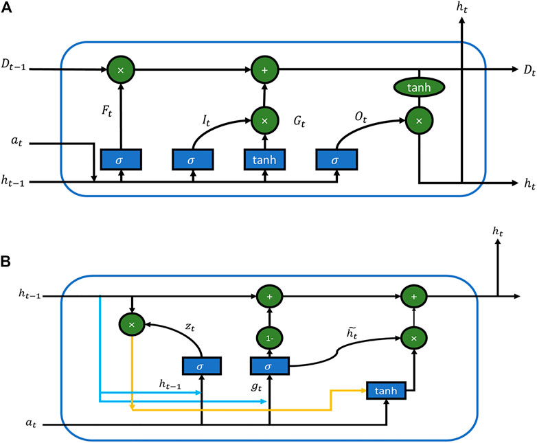
FIGURE 1. Parameter comparison between (A) LSTM framework and (B) GRU framework.

The activation of hidden unit at time step is processed as follows:

$r_t=\sigma \left(W_r{h}_{t-1}+ U_r{x}_t\right)(1)$

Initially, r_t is calculated using (1) where $\sigma$ represents logistic sigmoid function and W_r and U_r represent weight matrices. The new h_t is calculated by r_t with a tanh type layer:

$\widetilde{h_t}=\tanh \left(W\left(r_t\times h_{t-1}\right)+U{x}_t\right)(2)$

In GRU, $z_t$ replaces the remember gate along with the forget gate in LSTM. $z_t$ is calculated as follows:

$z_t=\sigma \left(W_z{h}_{t-1}+ U_z{x}_t\right)(3)$

Finally, the hidden state gets updated as follows:

$h_t=\left(1-z_t\right)\left(h_{t-1}\right)+ \left(z_t\right)\left(\widetilde{h_t}\right)(4)$

Data acquisition and preprocessing

In order to test imputation methods including KDR, IA, NIPALS, DA, and PMP, 2514 observations of six parameters, PM2.5, PM10, SO₂, NO₂, O₃, and CO were used from Guangzhou air quality governmental website (The World Air Quality Project, 2020). The collected data contained ∼2.5% missing values, and imputation was required with a suitable method. In order to select a suitable imputation method for this PM2.5 data, comparison experimentation was carried out. Firstly, all the rows with missing values were removed. The resulting new data were without missing values and run into random deletion of ∼2.5% values of variables PM2.5, PM10, SO₂, NO₂, O₃, and CO overall.

Secondly, imputation methods including KDR, IA, NIPALS, DA, and PMP were employed to fill the missing values. After imputation, the imputed data results were compared using numerical errors for the abovementioned imputation methods. The criterion RMSE (Eq. 5) helped in opting the outperformed technique.

$RMSE=\sqrt{\frac{{\left(x_{actual- x_{imputed}}\right)}^2}{N}}(5)$

Each method was allowed to iterate 5,000 times to impute missing data. The RMSE values obtained through comparison experimentation are tabulated in Table 1. KDR and TSR reported an RMSE value of 1.77 for overall imputed missing values. RSME values obtained by IA, NIPALS, and DA are 2.66, 3.6, and 2.25, respectively. Amongst all the methods, PMP showed better results with RMSE value equal to 1.22.

TABLE 1

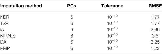
TABLE 1. Missing value imputation parameters

The outperformed method PMP was used to impute originally collected data. In order to summarize the impact of the individual variable on all other variables, correlation coefficients were obtained. For that, the correlation matrix was formed for imputed data that depicted the impact of individual input variables, i.e. PM10, SO₂, NO₂, O₃, and CO, in terms of correlation coefficients, on the output variable PM2.5 (Figure 2). The magnitude of the correlation coefficient shows the strength of correlation between two variables. The correlation matrix provided all possible correlations among all variables. Correlation coefficient ranges from −1 to +1. The coefficient value of −1 shows perfect inverse impact; 0 shows no impact, and +1 shows perfect direct impact. From the bottom left of Figure 2, it can be seen that output variable PM2.5 is strongly correlated with input variable PM10 with a coefficient value of 0.65. High coefficient value depicts that the change in concentration of PM10 will significantly affect the output variable PM2.5. Moreover, the output variable PM2.5 was least affected with the variation in SO₂ concentration that can be analyzed using the correlation coefficient in Figure 2. The correlation coefficient was very small, 0.07 between output variable PM2.5 and input variable SO₂. Removing SO₂ from the training data set for model training from the data under consideration would not significantly decrease the prediction performance of the model.

FIGURE 2

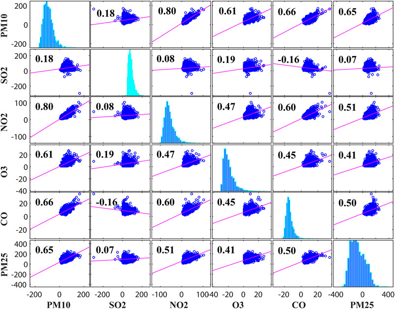
FIGURE 2. Matrix of correlation among all variables.

Moreover, the reported air pollutant safe limits (Agency, 2018) allow further analysis of the imputed data. A different coloring scheme with respect to the severity of individual pollutant concentration was employed to understand the distribution of data with their ranges (Table 2). The collected data contained approximately 80 months of PM2.5 and other pollutant data recorded on a per day basis.

TABLE 2

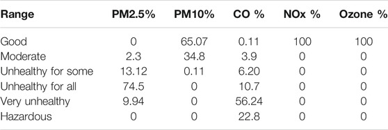
TABLE 2. Percentage wise data distribution in various ranges

Most of the PM2.5 data were found in an unhealthy range. Percentage-wise, data distribution in various ranges is given in Table 2. Out of 2514 total samples of PM2.5 collected for Guangzhou City, 0 samples were in green limit, 59 samples in yellow range, 330 samples in orange range, 1874 samples in red ranges, and 250 samples in purple range. PM10 data did not show much of the variation in ranges and categorized in safe or green ranges.

However, out of 2,514 total samples of PM10, 1,636 data points were in green range, 875 were in yellow, and 3 samples were in orange range that were collectively categorized in safe ranges. CO concentrations have shown variation in different ranges. Most of the data points were categorized in a not-safe range. Out of 2514 samples, three samples were in green range, 98 in yellow, 156 in orange, 269 in red, 1414 in purple, and 254 in maroon range. Moreover, most of the CO pollutant distributions were found in a very unhealthy range. NOx data and ozone data did not show any categorical variations. Almost all the data were in green range.

Methodology

The data were collected from the official Guangzhou air quality website that contained 2514 samples from Jan 2014 to Nov 2020 that contained missing values. To impute the missing values, various missing data imputation methods were employed and compared as shown in Table 1. This comparison study has been discussed in the Data acquisition and preprocessing section in detail. The imputation method giving the least RMSE was selected to impute the original missing data. After the data was imputed, in order to select the most correlated variables with PM2.5, a correlation matrix was formed as shown in Figure 2. According to the figure, SO₂ was found least correlated with PM2.5 with the correlation coefficient 0.07. Owing to the insignificant impact of the SO₂ on PM2.5 for the data under consideration, it was decided that SO₂ can be removed from the input variables list. Afterwards, prior to model training, data standardization was carried out using Eq. 6 to rescale the data for zero mean and unit variance. The standardized data were incorporated in model training where training input and corresponding output were termed as Xtrain and Ytrain. Training data with 2214 samples and validation data with 150 samples were devised for model training and validation, and 150 samples were devised for model testing. Furthermore, suitable parameters along with training data were employed to train these models, while the validation data were used to validate the model to check whether it is under-trained or over-trained. Subsequently, test data were fed to the trained model to evaluate the model prediction capability.

$\text{standardized} \left(x_i\right)=\frac{x_i-\mu }{\sigma }(6)$

where $x_i$ is the data value, $\mu$ represents the mean and σ represents standard deviation of the data. Moreover, RMSE, MAPE, and MEDAE were calculated using Eqs. 7, 8, and 9 respectively, to evaluate model performance by comparing PM2.5 predictions with actual PM2.5 from testing data.

$RMSE= \sqrt{\frac{1}{n}{\displaystyle \sum }_{i=1}^n{\left(x_i-pre{d}_i\right)}^2}(7)$

$MAPE=\frac{1}{n}{\displaystyle \sum }_{i=1}^n\left|\frac{x_i-pre{d}_i}{x_i}\right|(8)$

$MEDAE=\frac{1}{n}{\displaystyle \sum }_{i=1}^n\left|pre{d}_i-x_i\right|(9)$

Here, $x_i$, $pre{d}_i$, and $n$ represent actual PM2.5 value, predicted PM2.5 value, and testing data sample size, respectively.

LSSVM-based model development

Data standardization was done using Eq. 6 to scale it to zero mean and include unit variance in the data set. For LSSVM, two parameters, gamma and sigma, were selected after extensive trials, and set values came out to be 20 and 40, respectively.

LSTM-based model development

Input layer of LSTM contained four input units that were provided with training data to train the model. The training progressed using Adam algorithm. The Adam algorithm has the excellent capability to reach a globally optimal solution (Kingma and Ba, 2014). The Adam algorithm back-propagates the error to update the weights and biases of the LSTM to minimize the training error. Validation of the model training has also been performed to see if the model is under-trained or over-trained. The model was trained with 80 epochs. Moreover, necessary parameters for LSTM model training such as hidden units, dropout, initial learn rate, learn rate drop factor, learn rate, and drop period were set as 80, 0.9, 0.25, 1 × 10^–6, and 80, respectively. Finally, the test data were fed to obtain the prediction of the model.

Bi-LSTM-based model development

Bi-LSTM consists of two LSTMs that work in opposite direction, hence requiring more training time. The Adam algorithm was used to update the weights and biases of the Bi-LSTM to minimize the training error. The model was allowed to train for 80 epochs and validation of the model training was also carried out to see if the model was under-trained or over-trained. A dropout layer was also added to avoid overfitting while training the model. Moreover, necessary parameters for Bi-LSTM model training such as hidden units, dropout, initial learn rate, learn rate drop factor, and learn rate drop period were set as 80, 0.9, 0.75, 1 × 10^–6, and 80, respectively.

GRU-based model development

The GRU-based prediction model is shown in Figure 3. The GRU network trained the weights and biases while training to minimize the validation errors. The Adam algorithm was used for training due to its ability to reach the globally optimal solution effectively. The model was trained using 80 epochs and validation of the model training was also carried out to see if the model was under-trained or over-trained. A dropout layer was also added to avoid overfitting while training the model. If both training error and validation error decrease simultaneously, then the model is said to under-train. If training error decreases but validation error increases, the model is said to be over-trained. Moreover, necessary parameters for GRU model training such as hidden units, dropout, initial learn rate, learn rate drop factor, and learn rate drop period were set at 160, 0.9, 0.0009, 1, and 120, respectively.

FIGURE 3

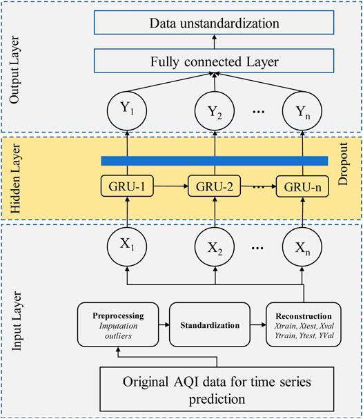
FIGURE 3. GRU-based prediction framework.

Results and discussion

The acquisition of the PM2.5 data was described in the Data acquisition and preprocessing section along with missing data handling. Amongst all the methods employed for the data considered, KDR and TSR performed better with ∼2.5% of missing value imputations (Table 1). Moreover, through imputation experiment, PMP was selected as the outperformed imputation method and, hence, used for the imputation of original collected PM2.5 missing data (Figure 4).

FIGURE 4

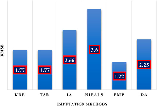
FIGURE 4. Missing values imputation method comparison.

This study has employed time series predictive RNN models such as LSTM, Bi-LSTM, and GRU for prediction of PM2.5 using input variables of PM10, NO₂, O₃, and CO. The models were compared and evaluated on prediction error. RSME, MAE, and MAPE model evaluation techniques were used to evaluate model prediction performance.

After preparing data for model training, LSSVM, LSTM, Bi-LSTM, and GRU models were developed for PM2.5 prediction. The training and testing performances of the respective models are discussed afterwards.

Training performance of models

All models were trained with 2214 samples of the input variables PM10, NO₂, O₃, and CO and output variable PM2.5. The training data comprised almost 74 months of data. The training performance, in terms of RMSE, of all the models are given in Table 3.

TABLE 3

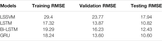
TABLE 3. Model performance review

LSSVM got trained with overall training RMSE of 29.4 (Figure 5A). The blue line in the upper graph shows the original values of PM2.5 of 74 months of data samples. The red line shows the trained PM2.5 values. It can be analyzed that the model training RMSE of 29.4 is significantly high. Moreover, the red-faced circles (Figure 6A) show the trained PM2.5 values in the form of scatter graph plotted against actual PM2.5 of 74 months of data. The red-faced circles were found distributed around the trend line (dashed diagonal line) and following it but not significantly, representing the deviation from the trend line at points. This was one of the reasons of high training RMSE, though the closeness of the red-faced circles with the trend line at various points also exhibits that the model was a good fit.

FIGURE 5

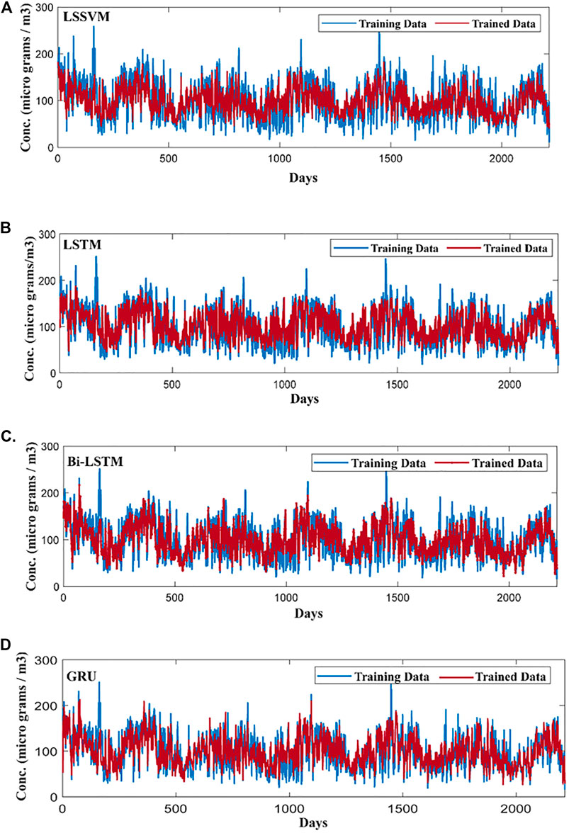
FIGURE 5. (A) LSSVM model PM2.5 prediction on training data. (B) LSTM model PM2.5 prediction on training data. (C) Bi-LSTM model PM2.5 prediction on training data. (D) GRU model PM2.5 prediction on training data.

FIGURE 6

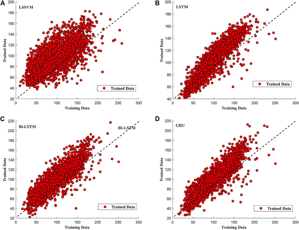
FIGURE 6. A) LSSVM training scatter plot. (B) LSTM training scatter plot. (C) Bi-LSTM training scatter plot. (D) GRU training scatter plot.

Seventy-four months of data were also employed to train the LSTM network, and training performance was plotted on a per day basis (Figure 5B). The solid blue line shows the actual PM2.5 from the training data and the red line shows the trained data by the model. It can be seen that model was able to learn the time series sequence very well and trained values showed relatively less RMSE 17.32.

Generally, it is not recommended to train the model as much in that trained values tightly fit the original data because overfitting takes away the generalizability of the model and future predictions get compromised drastically. Moreover Figure 6B was also plotted between original PM2.5 from 74 months of training data and trained data by the model. This scatter plot shows that the model was following the trend line with lesser deviation, which means the LSTM was able to learn time series sequence from the provided training data, and the closeness of red-faced circles with the trend line showed the superior learning capability of LSTM compared to LSSVM.

Figure 5C shows the training performance of the Bi-LSTM model with 74 months of PM2.5 training data. The upper plot shows the model has trained the time series sequences substantially from the provided training data. The Bi-LSTM model showed relatively poorer learning performance as compared to LSTM and showed the training RMSE of ∼19.29. However, the model trained the time series sequence very well and was also able to show good performance in learning training data values.

Overall, the model showed relatively larger training error at every instance of training than LSTM. Moreover, Figure 6C shows that the trained data are distributed around the trend line with lesser deviation than that of LSSVM but greater deviation than that of LSTM. However, the trained data were found following the trend line very well showing better time series sequence learning capability as compared to LSSVM but not better than LSTM.

The GRU network has fewer parameters to train as compared to LSTM and Bi-LSTM (Figure 1). The GRU training looks similar to the LSTM network (Figures 5B,D). However, comparison showed that GRU model trained better than previously discussed models from the 74 months of training data and reported training an RMSE value of 18.24. Figure 6D also shows that the trained data was spread along the trend line, depicting good time series sequence learning capability of the model comparable to LSTM.

Moreover, comparison of RMSE of the models for training data shows that LSTM outperforms. However, it is important to note that lesser RMSE while training might not necessarily give lesser RMSE while testing. After training, models were validated with 150 samples (January 2020–June 2020) and validation RMSEs were reported in Table 3. Validation performance figures can be found in Supplementary data.

Testing performance of models

All models were trained and tested with four variables discussed in the Data acquisition and preprocessing section. The test data set contained 150 samples from July 2020 to November 2020 (5 months). Prediction performance criteria i.e., RMSE, MAPE, and MEDAE of the models under consideration are tabulated in Table 4. For the first 2 months (July, August) of LSSVM model prediction, performance was a bit poor (Figure 7A). For the next 2 months (Sep, Oct), the model showed a good trend following ability compared to previous 2 months of results. However, the model was found deviating from the actual trend for the end of October and start of the final month (November). The model reported overall prediction error using testing data as RMSE, MAPE, and MEDAE equal to 17.94, 21.40, and 11.70 respectively. From (Figure 8A) the scatter plot of predicted values was visualized against the actual PM2.5 testing values. Red-faced circles showed that the predicted values were getting far apart along the trend line representing the poor performance of the model. The model was not generalized enough to predict the PM2.5 values accurately.

TABLE 4

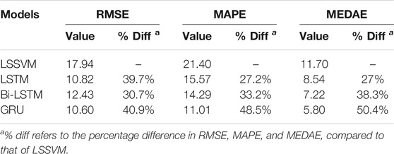
TABLE 4. PM2.5 models prediction errors with test data

FIGURE 7

FIGURE 7. (A) LSSVM model PM2.5 prediction on test data. (B) LSTM model PM2.5 prediction on test data. (C) Bi-LSTM model PM2.5 prediction on test data. (D) GRU model PM2.5 prediction on test data.

FIGURE 8

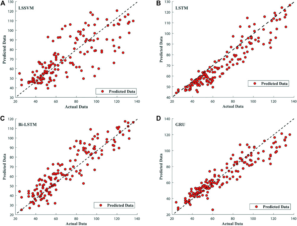
FIGURE 8. (A) LSSVM model test data scatter plot. (B) LSTM model test data scatter plot. (C) Bi-LSTM test data scatter plot. (D) GRU model test data scatter plot.

The testing performance of the LSTM model is shown in (Figure 7B). For the first 2 months, some prediction values were found less accurate but were following the actual trend. For next 2 months, the model prediction followed the actual trend very well and predicted values were very close to the actual trend. For very few points, the model compromised the prediction in these months. However, for the last month the LSTM PM2.5 model was found losing its outstanding trend following capability as it had shown in the previous 4 months Figure 8B shows the scatter plot of LSTM PM2.5 prediction against the actual testing values of PM25. The overall red-faced circles were found closely spread along the trend line compared to LSSVM representing good time series trend prediction of PM2.5 compared to that of the LSSVM model. The values of RMSE, MAPE, and MEDAE are 10.82, 15.57, and 8.54, respectively, which are 39.7%, 27.2%, and 27% lower than that of the LSSVM model, respectively, as shown in Table 4 and Figure 9.

FIGURE 9

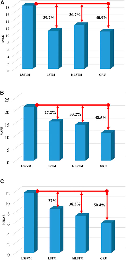
FIGURE 9. Model performance improvement summary. (A) RMSE improvement summary. (B) MAPE improvement summary. (C) MEDAE improvement summary.

In case of Bi-LSTM, the actual trend following the ability of the model is shown in Figure 7C. The Bi-LSTM model predicted PM2.5 values accurately and actual trend following for the first 2 months was even better than LSTM. For the next 2 months, the prediction capability of the Bi-LSTM model was reduced compared to LSTM model. Figure 8C shows the Bi-LSTM prediction scatter plot against the actual PM2.5 testing values. In terms of overall prediction, the red-faced circles were closely spread along with the trend line, however, a bit far compared to LSTM model scatter plot. The Bi-LSTM model produced RMSE, MAPE, and MEDAE as 12.43, 14.29, and 7.22, respectively, which are 30.7%, 33.2%, and 38.3% lower than that of the LSSVM model, respectively, as shown in Table 4 and Figure 9.

The GRU model with testing data set performed very well in terms of following the actual trend (Figure 7D). The model performance for the first 4 months of the testing data was significantly better than that of previously discussed models. The model displayed good prediction capability and followed the actual testing data trend accurately with close predicted values. However, for the last month the model lost excellent prediction performance but still predicted the actual trend effectively. However, in terms of overall prediction, the GRU model showed excellent performance with the testing data set as compared to previous models such as LSSVM, LSTM, and Bi-LSTM. Figure 8D shows the prediction performance of the GRU model in the scatter plot. The red-faced circles were found following the trend line excellently, better than that of LSSVM, LSTM, and Bi-LSTM.

The RMSE, MAPE, and MEDAE values are 10.60, 11.01, and 5.80 respectively, which are 40.9%, 48.5%, and 50.4% lower than those of the LSSVM model, respectively, as shown in Table 4 and Figure 9.

The performance criteria values of the GRU model are the lowest among comparative models considered in this work. The results depicted that the GRU model outperformed the other PM2.5 prediction models with the least RMSE, MAPE, and MEDAE.

Conclusion

In this study, predictions of PM2.5 in Guangzhou City in China were performed with different machine learning models including LSSVM, LSTM, Bi-LSTM, and GRU. Originally collected data contained missing values ∼2.5% of all data. Prior to model development, imputation experiment was run to shortlist the outperforming method among KDR, IA, NIPALS, DA, and PMP. Comparison experiment showed that PMP outperformed all other imputation methods with RMSE of 1.22. Therefore, the prediction models were developed in combination with PMP. The correlation result showed that SO₂ concentrations were badly correlated with PM2.5; therefore, the models were developed without SO₂ concentration in the data.

The RMSE, MAPE, and MEDAE of the LSSVM model with test data were produced to be 17.94, 21.4, and 11.7, respectively. Compared to LSSVM, the LSTM improved the prediction performance by 39.7% RMSE, 27.2% MAPE, and 27% MEDAE. In the case of Bi-LSTM, it improved the prediction performance by 30.7%, 33.2%, and 38.3% compared to that of LSSVM, according to RMSE, MAPE, and MEDAE, respectively. Likewise, GRU improved the prediction performance by 40.9%, 48.5%, and 50.4% compared to LSSVM, according to RMSE, MAPE, and MEDAE, respectively. Based on the prediction performance improvement percentages, it can be concluded that GRU in combination with PMP was able to update its learnable parameters better and outperformed the LSSVM, LSTM, and Bi-LSTM for the prediction of PM2.5 data from Guangzhou City, China.

Data Availability Statement

The original contributions presented in the study are included in the article/Supplementary Material; further inquiries can be directed to the corresponding authors.

Author Contributions

Conceptualization, FA; methodology, MS; software, MQ; formal analysis, NU; investigation, MS and MQ; writing — original draft preparation, MS; project administration, FA; writing — review and editing, NU and CS; supervision, FA. All authors have read and agreed to the published version of the manuscript.

Funding

This work was funded by the Higher Education Commission Pakistan (HEC) under the National Research Program for Universities (NRPU), 2017, Project Number 8167.

Conflict of Interest

The authors declare that the research was conducted in the absence of any commercial or financial relationships that could be construed as a potential conflict of interest.

Publisher’s Note

All claims expressed in this article are solely those of the authors and do not necessarily represent those of their affiliated organizations, or those of the publisher, the editors and the reviewers. Any product that may be evaluated in this article, or claim that may be made by its manufacturer, is not guaranteed or endorsed by the publisher.

Supplementary Material

The supplementary material for this article can be found online at: https://www.frontiersin.org/articles/10.3389/fenvs.2021.816616/full#supplementary-material

References

Agency, U. S. E. P. (2018). Technical Assistance Document for the Reporting of Daily Air Quality—the Air Quality Index (AQI). Geneva: World Health Orgaisation.

Google Scholar

Bigi, F., Haghighi, H., De Leo, R., Ulrici, A., and Pulvirenti, A. (2021). Multivariate Exploratory Data Analysis by PCA of the Combined Effect of Film-Forming Composition, Drying Conditions, and UV-C Irradiation on the Functional Properties of Films Based on Chitosan and Pectin. LWT. 137, 110432. doi:10.1016/j.lwt.2020.110432

CrossRef Full Text | Google Scholar

Brauer, M., Casadei, B., Harrington, R. A., Kovacs, R., Sliwa, K., Brauer, M., et al. (2021). Taking a Stand Against Air Pollution-The Impact on Cardiovascular Disease. J. Am. Coll. Cardiol. 77, 1684–1688. doi:10.1016/j.jacc.2020.12.003

CrossRef Full Text | Google Scholar

Bustreo, D. F. (2012). 7 Million Premature Deaths Annually Linked to Air Pollution. Geneva: World Health Orgaisation. Available at: https://www.who.int/mediacentre/news/releases/2014/air-pollution/en/#.WqBfue47NRQ.mendeley (Accessed December 20, 2019).

Google Scholar

Cai, X., Zhang, N., Venayagamoorthy, G. K., and Wunsch, D. C. (2004). “Time Series Prediction with Recurrent Neural Networks Using a Hybrid PSO-EA Algorithm,” in 2004 IEEE International Joint Conference on Neural Networks (IEEE Cat. No. 04CH37541), 1647–1652.

Google Scholar

Chen, Y., Cui, S., Chen, P., Yuan, Q., Kang, P., and Zhu, L. (2021). An LSTM-Based Neural Network Method of Particulate Pollution Forecast in China. Environ. Res. Lett. 16 (4), 044006. doi:10.1088/1748-9326/abe1f5

CrossRef Full Text | Google Scholar

Cho, K., van Merriënboer, B., Gulcehre, C., Bahdanau, D., Bougares, F., Schwenk, H., et al. (2014). Learning Phrase Representations Using RNN Encoder-Decoder for Statistical Machine Translation. Proceedings of the 2014 Conference on Empirical Methods in Natural Language Processing (EMNLP).

CrossRef Full Text | Google Scholar

Donald, J. K. (2021). “Atmospheric Chemistry: An Overview—Ozone, Acid Rain, and Greenhouse Gases,” in Building STEM Skills Through Environmental Education. Editors T. S. Stephen, and D. Janese (Hershey, PA, USA: IGI Global), 172–218.

Google Scholar

Dora, D. C. (2016). Air Pollution Levels Rising in many of the World’s Poorest Cities. Geneva: World Health Organisation. Available at: https://www.who.int/news/item/12-05-2016-air-pollution-levels-rising-in-many-of-the-world-s-poorest-cities (Accessed December 22, 2019).

Google Scholar

Fei, H., and Tan, F. (2018). Bidirectional Grid Long Short-Term Memory (BiGridLSTM): A Method to Address Context-Sensitivity and Vanishing Gradient. Algorithms. 11 (11), 172. doi:10.3390/a11110172

CrossRef Full Text | Google Scholar

Folch-Fortuny, A., Arteaga, F., and Ferrer, A. (2015). PCA Model Building with Missing Data: New Proposals and a Comparative Study. Chemometrics Intell. Lab. Syst. 146, 77–88. doi:10.1016/j.chemolab.2015.05.006

CrossRef Full Text | Google Scholar

Folch-Fortuny, A., Arteaga, F., and Ferrer, A. (2016). Missing Data Imputation Toolbox for MATLAB. Chemometrics Intell. Lab. Syst. 154, 93–100. doi:10.1016/j.chemolab.2016.03.019

CrossRef Full Text | Google Scholar

Gul, S., and Khan, G. M. (2020). “Forecasting Hazard Level of Air Pollutants Using LSTM’s,” in Artificial Intelligence Applications and Innovations. Editors I. Maglogiannis, L. Iliadis, and E. Pimenidis (Berlin: Springer International Publishing), 143–153.

CrossRef Full Text | Google Scholar

Hochreiter, S., and Schmidhuber, J. (1997). Long Short-Term Memory. Neural Comput. 9, 1735–1780. doi:10.1162/neco.1997.9.8.1735

PubMed Abstract | CrossRef Full Text | Google Scholar

Kampa, M., and Castanas, E. (2008). Human Health Effects of Air Pollution. Environ. Pollut. 151 (2), 362–367. doi:10.1016/j.envpol.2007.06.012

PubMed Abstract | CrossRef Full Text | Google Scholar

Kanner, J., Pollack, A. Z., Ranasinghe, S., Stevens, D. R., Nobles, C., Rohn, M. C. H., et al. (2021). Chronic Exposure to Air Pollution and Risk of Mental Health Disorders Complicating Pregnancy. Environ. Res. 196, 110937. doi:10.1016/j.envres.2021.110937

PubMed Abstract | CrossRef Full Text | Google Scholar

Karimian, H., Li, Q., Wu, C., Qi, Y., Mo, Y., Chen, G., et al. (2019). Evaluation of Different Machine Learning Approaches to Forecasting PM2.5 Mass Concentrations. Aerosol Air Qual. Res. 19, 1400–1410. doi:10.4209/aaqr.2018.12.0450

CrossRef Full Text | Google Scholar

Kim, H., Byun, G., Choi, Y., Kim, S., Kim, S.-Y., and Lee, J.-T. (2021). Effects of Long-Term Exposure to Air Pollution on All-Cause Mortality and Cause-specific Mortality in Seven Major Cities of South Korea: Korean National Health and Nutritional Examination Surveys with Mortality Follow-Up. Environ. Res. 192, 110290. doi:10.1016/j.envres.2020.110290

PubMed Abstract | CrossRef Full Text | Google Scholar

Kingma, D., and Ba, J. (2014). “Adam: A Method for Stochastic Optimization,” in International Conference on Learning Representations.

Google Scholar

Kumar, R., Kumar, P., and Kumar, Y. (2020). Time Series Data Prediction Using IoT and Machine Learning Technique. Proced. Computer Sci. 167, 373–381. doi:10.1016/j.procs.2020.03.240

CrossRef Full Text | Google Scholar

Kwak, S. K., and Kim, J. H. (2017). Statistical Data Preparation: Management of Missing Values and Outliers. Korean J. Anesthesiol. 70 (4), 407. doi:10.4097/kjae.2017.70.4.407

CrossRef Full Text | Google Scholar

Li, Y. (2021). Time-series Prediction Model of PM2.5 Concentration Based on LSTM Neural Network. J. Phys. Conf. Ser. 1861 (1), 012055. doi:10.1088/1742-6596/1861/1/012055

CrossRef Full Text | Google Scholar

Lin, X., Du, Z., Liu, Y., and Hao, Y. (2021). The Short-Term Association of Ambient fine Particulate Air Pollution with Hypertension Clinic Visits: A Multi-Community Study in Guangzhou, China. Sci. Total Environ. 774, 145707. doi:10.1016/j.scitotenv.2021.145707

PubMed Abstract | CrossRef Full Text | Google Scholar

Lu, F., Xu, D., Cheng, Y., Dong, S., Guo, C., Jiang, X., et al. (2015). Systematic Review and Meta-Analysis of the Adverse Health Effects of Ambient PM2.5 and PM10 Pollution in the Chinese Population. Environ. Res. 136, 196–204. doi:10.1016/j.envres.2014.06.029

PubMed Abstract | CrossRef Full Text | Google Scholar

Marriboyina, V. (2018). A Survey on Air Quality Forecasting Techniques. Geneva: World Health orgaisation.

Google Scholar

Oliveri Conti, G., Heibati, B., Kloog, I., Fiore, M., and Ferrante, M. (2017). A Review of AirQ Models and Their Applications for Forecasting the Air Pollution Health Outcomes. Environ. Sci. Pollut. Res. 24 (7), 6426–6445. doi:10.1007/s11356-016-8180-1

CrossRef Full Text | Google Scholar

Omer, A. (2018). LahoreSmog, Just How Bad Is it? [Online]. Lahore, Pakistan. Available at: https://medium.com/https://medium.com/pakistan-air-quality-initiative/lahoresmog-just-how-bad-is-it-81c0623cdb02 (Accessed December 20, 2020).

Google Scholar

Panda, R., and Maity, M. (2021). Global Warming and Climate Change on Earth: Duties and Challenges of Human Beings. Int. J. Res. Eng. Sci. Management. 4 (1), 122–125.

Google Scholar

Reddy, G. T., Reddy, M. P. K., Lakshmanna, K., Kaluri, R., Rajput, D. S., Srivastava, G., et al. (2020). Analysis of Dimensionality Reduction Techniques on Big Data. IEEE Access. 8, 54776–54788. doi:10.1109/access.2020.2980942

CrossRef Full Text | Google Scholar

Schuster, M., and Paliwal, K. K. (1997). Bidirectional Recurrent Neural Networks. IEEE Trans. Signal. Process. 45, 2673–2681. doi:10.1109/78.650093

CrossRef Full Text | Google Scholar

Sharma, J., Parsai, K., Raghuwanshi, P., Ali, S. A., Tiwari, V., Bhargava, A., et al. (2021). Emerging Role of Mitochondria in Airborne Particulate Matter-Induced Immunotoxicity. Environ. Pollut. 270, 116242. doi:10.1016/j.envpol.2020.116242

PubMed Abstract | CrossRef Full Text | Google Scholar

Siami-Namini, S., Tavakoli, N., and Namin, A. S. (2019). “The Performance of LSTM and BiLSTM in Forecasting Time Series,” in 2019 IEEE International Conference on Big Data (Big Data)), 3285–3292.

CrossRef Full Text | Google Scholar

Sosa, B. S., Porta, A., Colman Lerner, J. E., Banda Noriega, R., and Massolo, L. (2017). Human Health Risk Due to Variations in PM 10 -PM 2.5 and Associated PAHs Levels. Atmos. Environ. 160, 27–35. doi:10.1016/j.atmosenv.2017.04.004

CrossRef Full Text | Google Scholar

Sun, W., and Sun, J. (2017). Daily PM 2.5 Concentration Prediction Based on Principal Component Analysis and LSSVM Optimized by Cuckoo Search Algorithm. J. Environ. Manage. 188, 144–152. doi:10.1016/j.jenvman.2016.12.011

CrossRef Full Text | Google Scholar

The World Air Quality Project (2020). Air Pollution in Guangzhou: Real-time Air Quality Index Visual Map. Available at: https://aqicn.org/map/guangzhou (Accessed December 15, 2020).

Google Scholar

Walczak, B., and Massart, D. L. (2001). Dealing with Missing Data. Chemometrics Intell. Lab. Syst. 58 (1), 15–27. doi:10.1016/s0169-7439(01)00131-9

CrossRef Full Text | Google Scholar

Wang, K., Tong, Y., Yue, T., Gao, J., Wang, C., Zuo, P., et al. (2021). Measure-Specific Environmental Benefits of Air Pollution Control for Coal-Fired Industrial Boilers in China from 2015 to 2017. Environ. Pollut. 273, 116470. doi:10.1016/j.envpol.2021.116470

PubMed Abstract | CrossRef Full Text | Google Scholar

Wise, B., and Ricker, N. (1991). “Recent Advances in Multivariate Statistical Process Control: Improving Robustness and Sensitivity,” in Proceedings of the IFAC. ADCHEM Symposium: Citeseer, 125–130.

Google Scholar

World Health Organization (2021). Air Pollution [Online]. Available at: https://www.who.int/health-topics/air-pollution (Accessed November 13, 2020).

Google Scholar

Wu, J.-Z., Ge, D.-D., Zhou, L.-F., Hou, L.-Y., Zhou, Y., and Li, Q.-Y. (2018). Effects of Particulate Matter on Allergic Respiratory Diseases. Chronic Dis. translational Med. 4 (2), 95–102. doi:10.1016/j.cdtm.2018.04.001

CrossRef Full Text | Google Scholar

Xing, Y. F., Xu, Y. H., Shi, M. H., and Lian, Y. X. (2016). The Impact of PM2.5 on the Human Respiratory System. J. Thorac. Dis. 8 (1), E69–E74. doi:10.3978/j.issn.2072-1439.2016.01.19

CrossRef Full Text | Google Scholar

Zhang, L., Morisaki, H., Wei, Y., Li, Z., Yang, L., Zhou, Q., et al. (2019). Characteristics of Air Pollutants inside and Outside a Primary School Classroom in Beijing and Respiratory Health Impact on Children. Environ. Pollut. 255, 113147. doi:10.1016/j.envpol.2019.113147

PubMed Abstract | CrossRef Full Text | Google Scholar