Land Use Zoning Management to Coordinate the Supply–Demand Imbalance of Ecosystem Services: A Case Study in the City Belt Along the Yellow River in Ningxia, China

1 Introduction

Ecosystem services (ESs), the direct and indirect goods and services provided by ecosystems to human society, can effectively bridge the natural environment and human society (Costanza et al., 1997; Wang et al., 2017; Huang et al., 2020). Studies show that ecosystems can only provide limited ESs, while human society has increased demand for ESs, driven by rapid population growth and socioeconomic development, especially in developing countries (Birge et al., 2016; Wei et al., 2017). Almost 60% of the global ecosystem is deteriorating at an unprecedented rate, caused by the surpassing of demand compared to supply and their spatial mismatches (MEA, 2005; Bagstad et al., 2013). Therefore, how to effectively manage ecosystems to minimize the supply–demand mismatches of ESs is critical for improving human well-being and sustainable development (Furst et al., 2013; Chang et al., 2021).

An ecosystem can provide multiple ESs simultaneously, while ESs are not independent of each other, as they may be related to the same ecological process or influenced by the same socioecological factors (Meacham et al., 2016). Complex relationships exist among multiple ESs, especially the tradeoff that one ES decreases with the increase of another ES, which is the main challenge in improving multiple ESs simultaneously (Spake et al., 2017; Peng et al., 2019b). Understanding the interactions among multiple ESs and their socioecological driving mechanisms has been proven to be useful and critical in developing management policies related to land use, vegetation restoration, and spatial planning (Chen et al., 2019; Schirpke et al., 2019). Fu et al. (2017) provided management suggestions for different subregions by analyzing the impacts of land use change and climate change on ESs, such as planting grasslands with high coverage in the oasis zone and establishing protected areas in the mountain and desert zones. However, most existing studies have focused on the supply side but neglected the demand side, which has a closer connection to human society (Meng et al., 2020; Chang et al., 2021).

Existing studies have suggested that not only the ES supply–demand match degree but also their relationships would change with different socioecological contexts (Xu et al., 2017; Sun et al., 2019). For example, three ESs of crop production, climate regulation, and recreation had higher demand in cropland and urban areas but higher supply in natural forests and olive orchards (Lorilla et al., 2019). Crop production and carbon sequestration represent tradeoffs in mountain regions but synergy in plain irrigation areas (Zhou et al., 2017; Lyu et al., 2019). Thus, zoning management would be an effective method to improve human well-being while maintaining ecosystem function and resilience, especially for regions with high spatial heterogeneity (Xu L.-X. et al., 2019; Zeng et al., 2020; Chang et al., 2021). Most existing studies tended to classify zones through either environmental characteristics or ecological function and ESs. The former classification is mainly based on natural ecological features and scarcely considers the role of humans in the ecosystem (Xu et al., 2020; Yu et al., 2021). The latter classification is beneficial to identify the ecological problem and optimization goal but fails to consider the socioecological contexts and make niche-targeting suggestions. For example, both excess fertilizer in plain irrigation and lack of riparian buffer could result in water pollution; thus, different suggestions should be made for different regions for water purification (Lyu et al., 2019). Till now, rare studies have combined natural ecological features and ESs to divide the management zones.

ES bundles, sets of ESs that repeatedly appear together across space or time, can effectively represent the spatial heterogeneity of ESs and their interactions (Raudsepp-Hearne et al., 2010; Cord et al., 2017). In this study, we proposed a new framework to classify ecological zones and propose management suggestions for the identified problems by quantifying the status of ES supply–demand, their bundles, and socioecological drivers. The City Belt along the Yellow River in Ningxia (CBYN), located in the upstream part of the Yellow River basin, has a fragile ecological environment with various landscape types—deserts, oases, and mountains. CBYN faces severe conflict between rapid socioeconomic development and ecological protection. In this study, taking CBYN as the study area, we quantified the supply and demand of five critical ESs, identified their interactions and socioecological driving mechanisms, classified the ecological zones, and provided specific suggestions. This study aimed to 1) estimate the supply–demand status of multiple ESs in a spatially explicit manner; 2) clarify ES tradeoffs/synergies and their driving mechanisms at different sides; and 3) develop a comprehensive approach to combining the socioecological environment and ESs into zoning management. The results are expected to provide a scientific foundation for land use planning and decision-making for sustainable ecosystem management.

2 Materials and Methods

2.1 Study Area

Located in the northwestern Ningxia Hui Autonomous Region, China, the CBYN (36°54′30″–39°23′23″N, 104°17′7″–106°58′13″E) covers approximately 22,000 km² at the intersection of the Loess Plateau, the Mongolian Plateau, and the Tibetan Plateau (Figure 1). It borders the Tengger, Maowusu, and Ulanbuh deserts in the west, east, and north directions, respectively, with elevations ranging from 956 to 3,544 m. It has a continental climate characterized by low precipitation, abundant sunshine, high evapotranspiration, and four distinct seasons of a late windy spring, short summer, early autumn, and long cold winter. The average annual precipitation in 1989–2017 was 191.38 mm, which falls mostly in June–August, with an average annual temperature of 10.38°C. The Yellow River flows from southwest to northeast through Zhongwei City, Wuzhong City, Yinchuan City, and Shizuishan City, fostering the formation of irrigation for agricultural production and providing abundant water resources for human life, agriculture, and industrial production.

FIGURE 1

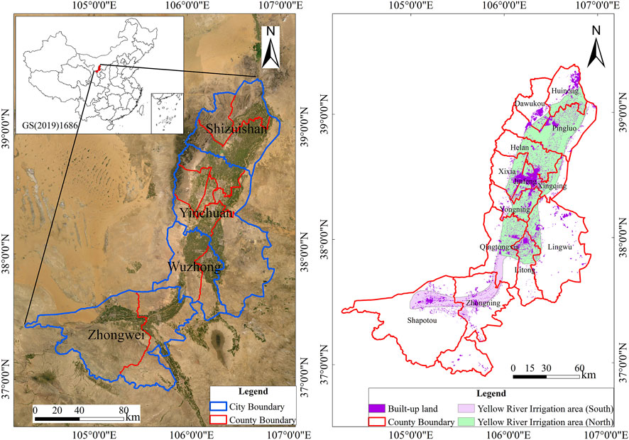
FIGURE 1. Location of the study area.

Driven by global climate change and rapid socioeconomic development, several ecological problems have emerged in the CBYN, such as food security, water pollution, and global warming. Unique landscapes and a rich cultural background also generate abundant tourism resources in the CBYN. Thus, based on ecological problems, data availability, and the feasibility of assessment methods, four ESs with high relevance to stakeholder welfare were selected, including one provision service (crop production), two regulating services (carbon sequestration and nutrient retention), and one cultural service (recreational opportunity). The main datasets used in this study are listed in Table 1.

TABLE 1

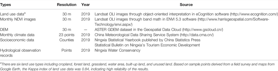
TABLE 1. Sources of the primary data.

The spatial distribution of population, a critical and essential factor in calculating ES demand, was simulated through census data at the county scale and for influencing factors using the random forest model. First, the influencing factors of population distribution were selected through a literature review (Qi et al., 2015; Stevens et al., 2015; Tan et al., 2017), including elevation, slope, distance to water, distance to the Yellow River, distance to transportation, distance to railways, distance to roads at the province level, distance to the city center, built-up percentage. These factors were resampled to 30 m. Next, the relationship between population density and the average value of influencing factors at the county level was explored through a random forest model, in which the explained variance of the derived model reached 88.24%. Thus, the established random forest model could effectively simulate population spatialization. At last, a population distribution map at 30 m was generated based on the derived model and the distribution maps of the influencing factors. The details are listed in Supplementary Material Section S1.

2.2 Methodology

This study was conducted in four steps. First, the supply and demand of five key ESs (crop production, carbon sequestration, nutrient retention, sand fixation, and recreational opportunity) were quantified in a spatially explicit manner. Second, interactions among the ESs were quantified at three sides of supply, demand, and match degree through correlation analysis and a self-organizing map (SOM) method. Third, the socioecological driving mechanisms were explored for the supply and demand of each ES through random forest analysis and the SOM method. Fourth, zoning management and corresponding measures were proposed by combining ES bundles and socioecological driver clusters. The technical roadmap is shown in Figure 2.

FIGURE 2

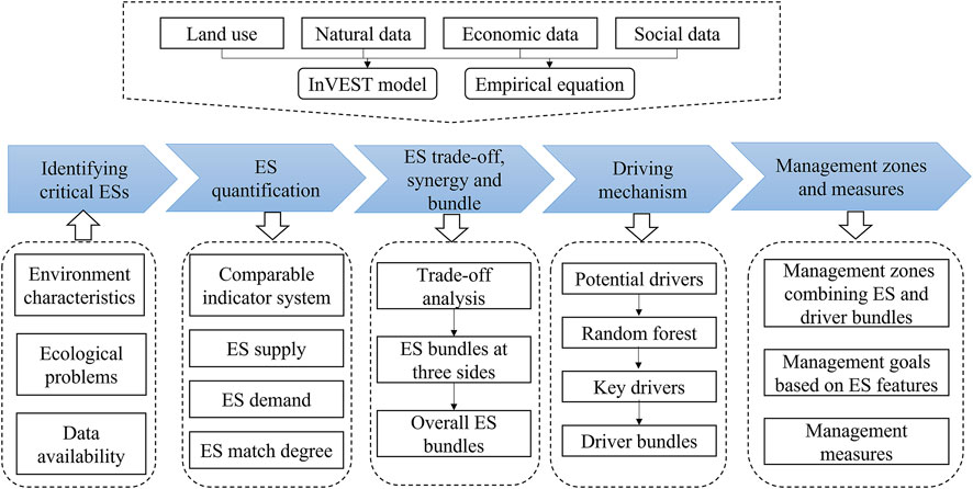
FIGURE 2. Framework for dividing management zones and proposing measures based on ES supply–demand, tradeoffs, and environmental characteristics.

2.2.1 Mapping ES Supply and Demand

The flat topography and opulent sunshine in the CBYN provide favorable conditions for agricultural production (Lyu et al., 2018). Thus, it has become one of the most critical grain production bases in northwestern China but also suffers from serious nonpoint pollution (Dong and Ma, 2012; Li et al., 2017). The CBYN is surrounded by deserts on three sides, while Helan Mountain provides great benefits in preventing wind erosion and sandstorms (Xu J. et al., 2019). Carbon sequestration and emission play a critical role in mitigating global warming (Ito et al., 2016). Besides that, a multiethnic culture and unique landscape provide the CBYN with abundant opportunities for ecotourism (Zhou and Yan, 2009; Lyu et al., 2018). According to the environmental characteristics, ecological problems, method feasibility, and data availability in the CBYN, the following five ESs were selected and estimated at a spatial resolution of 30 m in 2019: one provision service of crop production, three regulating services of carbon sequestration, nutrient retention, and sand fixation, and one cultural service of recreational opportunity.

2.2.1.1 Crop Production

The supply of crop production was calculated based on the statistical data of the main crop output at the county scale obtained from the Ningxia Statistical Yearbook, including rice, wheat, corn, tubers, and soybeans. By referencing the method used by Hu et al. (2018), the crop output value was allocated to cropland at the grid scale (30 m) based on the linear relationship between crop yield and NDVI. It was calculated from Eq. 1:

$S_{CPi}=\frac{NDV{I}_i}{NDV{I}_{sum}}\times G_{sum}(1)$

where S_CPi is the supply of crop production in pixel i (kg), G_sum is the total crop output in each county, NDVI_i is the normalized NDVI value in pixel i, and NDVI_sum is the sum of the normalized NDVI value in cropland for each county.

The demand for crop production was calculated through the per capita food demand and population distribution. According to the per capita food demand based on the average grain pattern of China and the Ningxia Statistical Yearbook, the annual consumption of major foods by urban and rural households is 112.1 kg per capita. It was calculated as follows:

$D_{CPi}=PO{P}_i\times 112.1(2)$

where D_CPi is the demand for crop production in pixel i (kg), and POP_i is the population in pixel i.

2.2.1.2 Carbon Sequestration

The supply of carbon sequestration was estimated through the net primary productivity (NPP) (Zhou et al., 2017), which was calculated through the CASA model as follows:

$NPP=APAR\times \epsilon (3)$

$ARAR=SOL\times FPAR\times 0.5(4)$

$\epsilon =T_{\epsilon 1}\times T_{\epsilon 2}\times W_{\epsilon }\times {\epsilon }_{max}(5)$

where NPP is the net primary productivity, APAR is the canopy-absorbed incident solar radiation over a time period (MJ/m²), ε is the light utilization efficiency (gC/MJ), SOL is the total solar radiation (MJ/m²), FPAR is the canopy-absorbed fraction of photosynthetically active radiation, $T_{\epsilon 1}$ and $T_{\epsilon 2}$ are temperature stress coefficients, $W_{\epsilon }$ is a water stress coefficient, and ${\epsilon }_{max}$ is the maximum light-use efficiency of vegetation (gC/MJ). For related parameters, refer to Zhu et al. (2007).

The demand for carbon sequestration was assessed by carbon emissions in the ecosystem, mainly coming from industrial fossil-fuel consumption, human respiration, cropland soil respiration, and livestock farming. It was calculated as follows:

$D_{CS}=C_i+C_h+C_l+C_c(6)$

$C_I=Outpu{t}_I\times F_I(7)$

$C_P=POP\times F_P(8)$

$C_L=N_{Lj}\times W_{Lj}\times F_{Lj}(9)$

$C_C=S_c\times F_C(10)$

where D_CS is the total carbon emissions by ecosystem (tC/a), and C_I, C_P, C_L, and C_C are the carbon emissions caused by industrial production, human respiration, livestock farming, and cropland soil respiration, respectively. $Outpu{t}_I$ is the industrial output value in each county, and F_I is the carbon emission ratio for industrial output (0.54 tC/10000 yuan) (Cui et al., 2019). POP is the population, and F_P is the carbon emission factor per person per year (0.13797 tC) (Zhang et al., 2014). Sc is the area of cropland (km²), and F_C is the carbon emission factor (tC/km²) (Li et al., 2010). N_Lj is the number of ith livestock, W_Lj is the live weight of ith livestock (kg), and F_Lj is the carbon emission factor per kilogram of ith livestock (Zhang et al., 2014) (Table 2). For the spatialization of carbon emissions, C_I and C_L in each county were allocated equally into the built-up land and grassland, respectively.

TABLE 2

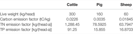
TABLE 2. Carbon and nutrient emission factors of livestock in the CBYN.

2.2.1.3 Nutrient Retention

The supply of nutrient retention refers to the contribution of vegetation and soil to water purification through the removal of nonpoint nutrient pollutants from runoff. It was calculated through the InVEST NDR model with input data of topography, surface runoff, land use type, pollution load, and empirical parameters derived from relevant literature (Redhead et al., 2018). It was assessed as follows:

$N{E}_i=AL{V}_i\times f_j(11)$

$AL{V}_i=\frac{{\lambda }_i}{{\lambda }_{\overline{w}}}\times po{l}_i(12)$

where NE_i is the nutrient retention amount in pixel i (kg/pixel), f_j is the retention capacity of land use j, ALVi is the adjusted loading value in pixel i, poli is the exported coefficient in pixel i, λ_i is the runoff index in pixel i, and ${\lambda }_{\overline{w}}$ is the mean runoff index.

For the model calibration and validation, data on nitrogen concentration, phosphorus concentration, and river flow in three gauging stations were derived from Ningxia Water Conservancy. Annual nutrient retention was calculated through the nutrient load difference between the inlet and outlet in the basin; then, it was compared to simulated data from the InVEST NDR model, indicating the high reliability of the simulation results for nitrogen retention but low reliability for phosphorus retention (Supplementary Figure S3). As the amount of nitrogen retention was nearly 10 times that of phosphorus retention, the underestimation of phosphorus retention did not significantly impact the accuracy of the overall assessment of nutrient retention.

The demand for nutrient retention was assessed by nonpoint nutrient emission from an ecosystem including total nitrogen (TN) and total phosphorus (TP), mainly including three sources: agricultural production, human living, and livestock breeding.

$D_{NR}=N{E}_C+N{E}_P+N{E}_L(13)$

$N{E}_C=S_C\times R_C(14)$

$N{E}_P=W_P\times R_P(15)$

$N{E}_L=N_{Lj}\times R_{Lj}(16)$

where D_NR is the total nutrient emission by ecosystem in each pixel (kg/a), and NE_C, NE_P, and NE_L are the nutrient emissions caused by agricultural production, human living, and livestock farming, respectively. Sc is the area of cropland (km²), and F_C is the nutrient emission factor of cropland [19.04 kg/(km²·a) of TN and 0.75 kg/(km²·a) of TP] (Yinlu Yang et al., 2011). W_P is the wastewater discharge from daily life (L), and R_P is the nutrient emission factor of wastewater (23.02 mg/L of TN and 3.74 mg/L of TP) (Yinlu Yang et al., 2011). N_Lj is the number of ith livestock, and R_Lj is the nutrient emission factor of ith livestock [kg/(head·a)] (Yinlu Yang et al., 2011) (Table 2). For the spatialization of carbon emissions, NE_L in each county was equally allocated to grassland, while NE_P in each county was allocated to built-up land based on the population distribution.

2.2.1.4 Sand Fixation

Wind erosion, the root cause of desertification in arid and semiarid regions, decreases soil productivity and threatens human health and ecological safety (Su et al., 2020). The ecosystem could reduce it through surface vegetation, steep slopes, and low soil erodibility. The supply and demand of sand fixation were calculated through the Revised Wind Erosion Equation. This method can comprehensively consider the impacts of climate variability, topography, soil contexts, and vegetation coverage. The supply and demand of sand fixation were assessed as follows:

$\mathrm{\Delta }Q=Q_0-Q_v(17)$

$Q\left(x\right)=Q_{max}\left\{1-\text{exp}\left[-{\left(\frac{x}{S}\right)}^2\right]\right\}(18)$

$Q_{max}=109.8\times WF\times EF\times K\times SCF\times VC(19)$

$S=150.71\times {\left(WF\times EF\times K\times SCF\times VC\right)}^{-0.3711}(20)$

where $\mathrm{\Delta }Q$ is the supply amount of sand fixation [t/(ha·yr)], $Q_0$ is the potential soil erosion without vegetation coverage [t/(ha·yr)], $Q_v$ is the actual soil erosion under current coverage and management and the demand amount of sand fixation [t/(ha·yr)], $Q\left(x\right)$ is the amount of soil transported by the wind past a point x, Q_max is the maximum amount of soil at downwind, S is the critical filed length at which the transported soil is 63.2% of Q_max, WF is the weather factor calculated based on wind speed, air density, soil wetness, and snow cover factor, EF is the erodible fraction calculated through soil contexts, SCF is the soil crust factor calculated through soil clay and organic matter content, K is the soil roughness factor calculated, and VC is the vegetation coverage factor. For details, see Jiang et al. (2016).

2.2.1.5 Recreational Opportunity

The supply of recreational opportunity refers to the potential for recreation and ecotourism provided by an ecosystem. It was calculated by the characteristics, properties, and potential activities of the landscape, including four types of indicators: accessibility, tourism aptitude, scenic beauty, and civilization (Tables 3 and 4) (Nahuelhual et al., 2017). The relative weights of each indicator were calculated through the analytical hierarchy process based on interviews with 15 academics and postgraduate students familiar with the tourism industry in the study area. All the raster maps were first normalized to 0–100 and then summed up with their weights to calculate the supply amount.

TABLE 3

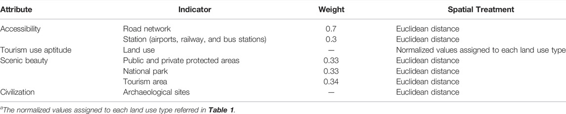
TABLE 3. Attributes, variables, and weights used to assess the supply of recreational opportunities.

TABLE 4

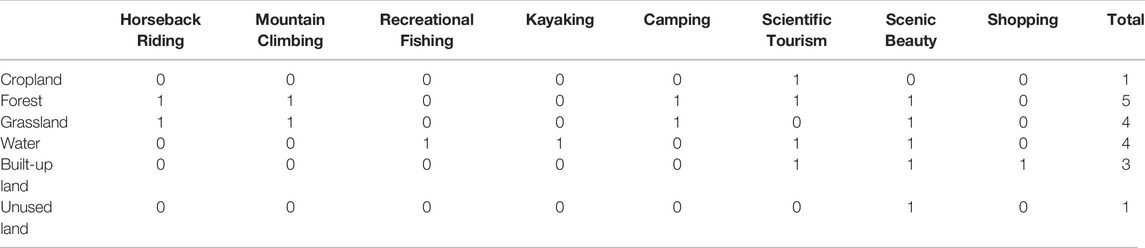
TABLE 4. Potential activities in each land use type in the CBYN.

The demand for recreational opportunities was assessed by the distribution of beneficiaries, including residents and tourists. The number of tourists was derived from the Statistical Bulletin on Ningxia’s Tourism Economic Development in 2019. The number of tourists was firstly divided into each county based on the distribution and level of tourist attractions and then equally allocated to built-up land in each county. It was converted into permanent resident equivalent by dividing by the number of nights (365) and added to the raster map of residents. At last, the demand for recreational opportunity was simulated by the rescaled addition map from 0 (low) to 1 (high).

2.2.2 Calculation of Spatial Mismatches Between Supply and Demand for Each ES

The ecological supply–demand ratio was used to quantify the degree of spatial match between the supply and demand of different ESs, as is widely done in similar studies (Cui et al., 2019; Lorilla et al., 2019). It was calculated as follows:

$\text{ESDR}=\frac{S-D}{\left(S_{max}+D_{max}\right)/2}(21)$

where S and D are the supply and demand of each ES, respectively, and S_max and D_max are the maximum values of supply and demand for a specific ES. A positive value of ESDR indicates that the supply of a specific ES is larger than its demand; a negative value indicates that the supply does not meet its demand, while a value of zero means that its supply and demand are balanced.

2.2.3 Analysis of ES Interactions and Bundles

Spearman correlation analysis and principal component analysis (PCA) were used to investigate the interactions among the ESs. The SOM method was used to identify ES bundles, while the optimal number of clusters was determined according to the results of PCA and NbClust functions. The above analyses were performed by differentiating supply, demand, and the match degree through the “raster,” “corrgram,” “psych,” “NbClust,” and “kehonen” packages in the R statistical software (https://www.r-project.org/).

2.2.4 Exploring the Socioecological Driving Mechanism of ES Supply and Demand

First, we identified critical driving factors for ES supply and demand from a complex socioecological environment through random forest analysis. The potential socioecological driving factors of ES supply and demand were collected from five sources: public recognition, expert knowledge, ES assessment, environmental characteristics, and relevant literature (Hauck et al., 2015; Mouchet et al., 2017; Spake et al., 2017; Li and Wang, 2018; Lyu et al., 2018; Lyu et al., 2019). Twenty potential factors were originally selected (Table 5). To avoid multicollinearity, Pearson’s correlation analysis was first applied to all the variables, and the results showed that there were no high correlations among them. Then, the random forest model was applied to identify the most important factors for the supply, demand, and match degree of each ES, which was performed in the “randomForest” package in the R software. Fourteen factors were finally selected that could effectively simulate the spatial heterogeneity of the supply, demand, and match degree of the four ESs (Table 5). To explore the socioecological background of ES mismatches and bundles, these 14 driving factors selected were clustered based on their similarities in spatial distribution using the SOM clustering method, which was performed using the “kohonen” and “raster” packages in the R software. Then, driving factor clusters were overlaid with ES bundles to investigate the socioecological context of the ES bundles.

TABLE 5

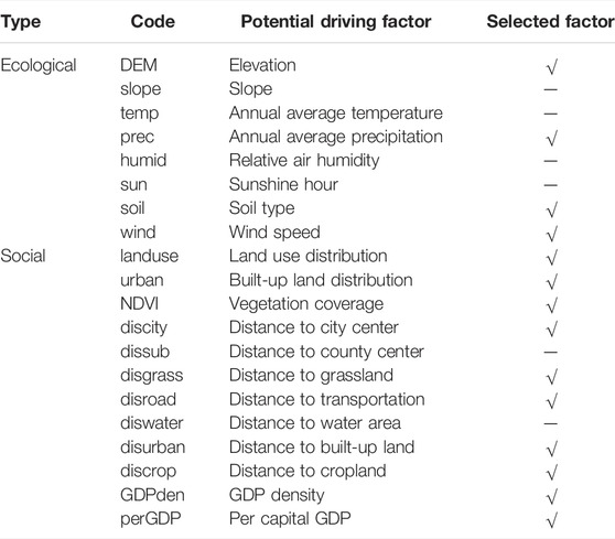
TABLE 5. Potential and selected driving factors for ES supply, demand, and match degree.

2.2.5 Zoning Management Based on ES Bundles and Socioecological Driver Clusters

In our study, zoning management combined ES characteristics and the socioecological environment, which was convenient to put forward measures of ecosystem management and achieve the goal of sustainable supply of multiple ESs. First, ES bundles for all the three components (supply, demand, and supply–demand match degree) in Section 2.2.2 and driver clusters in Section 2.2.3 were overlaid to propose management zones. Second, based on the characteristics of ES supply, demand, and match degree, and the interactions among ESs, we identified the main ecological problem and optimization objective. Then, combining the different socioecological conditions that had significant impacts on ESs, management measures were proposed to achieve the management goals. In specific, management zones less than 1,000 km² were eliminated, and there were 14 zones in total.

3 Results

3.1 Spatial Distribution of ES Supply and Demand

Significant differences existed in the spatial distribution of ES supply, demand, and match degree (Figure 3). Among the three sides of ESs, supply and match degree had a similar pattern for each ES, while higher supply only partly overlapped with higher demand for the five ESs except crop production. The total supply of crop production in the CBYN reached 223.52 × 10⁷ kg in 2019, much higher than its total demand of 50.84 × 10⁷ kg, suggesting the critical role of the CBYN as a crop production base. The unsatisfied demand for crop production was mainly distributed in urban and rural areas with human settlements, while its excess supply was mainly distributed in cropland in the central plain, with lower excess supply in Dawukou District. For carbon sequestration, its total supply (173.61 × 10¹⁰ gC) was far less than its total demand (950.61 × 10¹⁰ gC), while excess supply was mainly located in the forest land, with unsatisfied demand in urban and rural areas. The total supply of nutrient retention reached 2.17 × 10⁷ kg, which was lower than the total demand of 3.13 × 10⁷ kg. Its excess supply mainly lied in the croplands in Xixia District, Jinfeng District, Xingqing District, Dawukou District, Huinong District, and Lingwu City, while the unsatisfied demand was located in urban and rural areas and in grassland with low vegetation coverage in the north region. For sand fixation, its total supply (8.686 × 10⁸ t/ha) was lower than its total demand (10.871 × 10⁸ t/ha), resulting in the occurrence of sand and dust storms and further threatening human well-being, especially in the transition region between the central plain and the fringe mountains without vegetation coverage. For recreational opportunity, the unsatisfied demand was mainly in the south fringe area with low accessibility and low aesthetics, while the excess supply was in the areas with natural beauty and forest gardens.

FIGURE 3

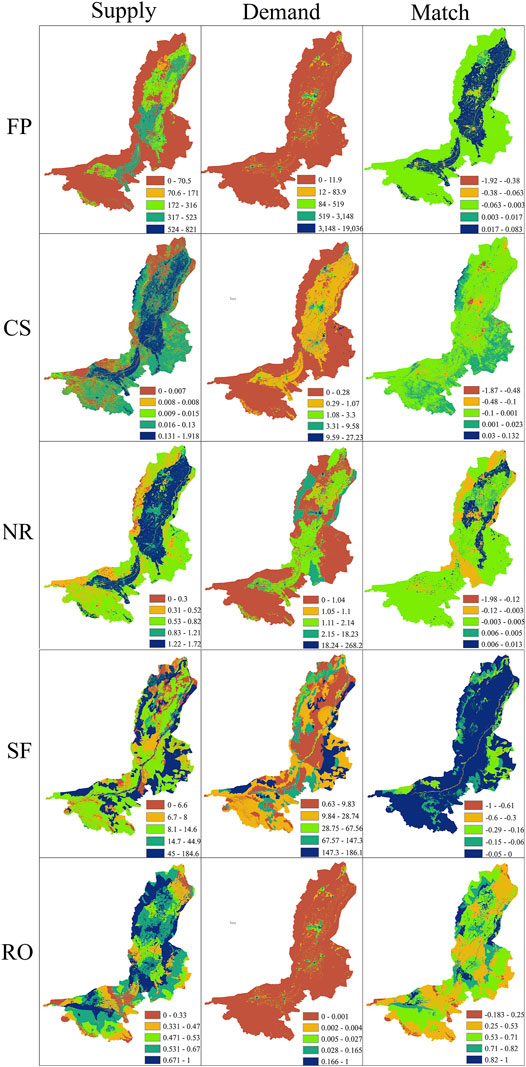
FIGURE 3. Spatial distribution of ES supply, ES demand, and ESDR in 2019.

3.2 Interactions Among ESs Based on Supply, Demand, and Match Degree

3.2.1 Correlation Coefficients Among ESs in Different Sides

Spearman’s correlation coefficients of paired ESs were different among the three sides of supply, demand, and match degree (Figure 4). Among the 10 pairs of ESs, only one pair (crop production and nutrient retention) exhibited consistent synergies with different strengths across the three sides. Three pairs (crop production vs carbon sequestration, carbon sequestration vs nutrient retention, sand fixation vs nutrient retention) exhibited opposite correlations between the supply and demand sides and the match side. Sand fixation and other ESs exhibited weak correlations at the supply and demand sides but strong synergies with crop production and nutrient retention and strong tradeoffs with carbon sequestration and recreational opportunity. Recreational opportunity and the other three ESs (crop production, carbon sequestration, and nutrient retention) exhibited strong tradeoff relationships at the supply side, but showed synergy relationships at demand side.

FIGURE 4

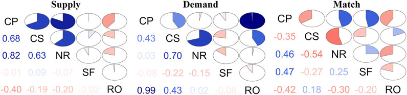
FIGURE 4. Correlation coefficients among ESs at three sides of supply, demand, and match degree (blue for positive correlation, red for negative correlation; CP—crop production, CS—carbon sequestration, NR—nutrient retention, SF—sand fixation, RO—recreational opportunity).

3.2.2 Spatial Distribution and Characteristics of ES Bundles

As indicated by the results of PCA (Figure 5) and the Calinski criterion of the K-means clustering method, 3, 3, 3, and 6 bundles were suggested for the five ESs at supply, demand, match degree, and all the three above components, respectively (Figure 6). At the supply side, the central plain covered by cropland (ESB 3) could provide higher levels of crop production, carbon sequestration, and nutrient retention but lower levels of the other two ESs. The transition region between the central plain and the fringe area with lower vegetation coverage (ESB 3) provided higher levels of sand fixation but lower levels of the other ESs; the fringe area and central built-up land (ESB 2) mainly provided higher recreational opportunity. At the demand side, the central urban and rural areas (ESB 3) had the highest demand for the discussed ESs except for sand fixation, while the transition region between the central plain and the fringe area with lower vegetation coverage (ESB 1) had the highest demand for sand fixation. At the supply–demand match degree side, the urban and rural areas (ESB 3) exhibited the lowest match degree for crop production, carbon sequestration, and nutrient retention but the highest match degree for recreational opportunity; the transition region had the lowest match degree for sand fixation. For all the three sides of these five ESs, the whole region can be divided into six regions, with different characteristics in ES supply, demand, and match degree. The inner urban and rural areas had the highest demand and lowest match degree of the discussed ESs except for sand fixation among the whole region, while the outer urban and rural areas had lower demand and higher match degree compared to the inner urban and rural areas. In specific, the outer urban and rural areas had the highest match degree of recreational opportunity across the whole region. ESB 2 and ESB 5 are both located in the central cropland with the highest supply of crop production, carbon sequestration, and nutrient retention, while ESB 5 also had the highest supply of sand fixation.

FIGURE 5

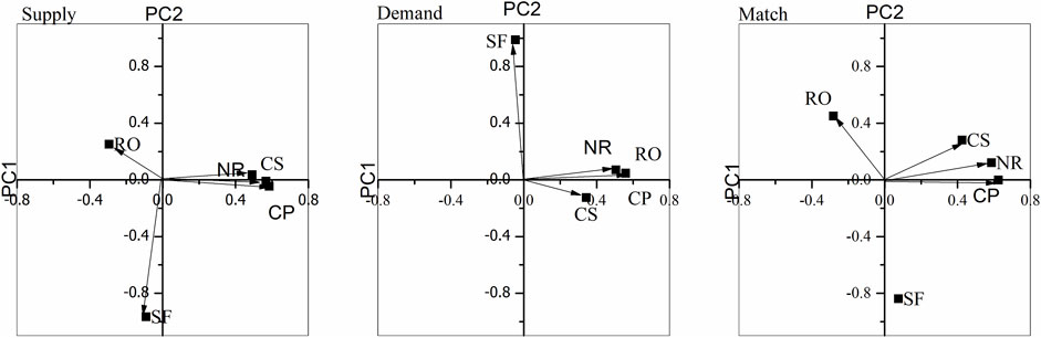
FIGURE 5. Principal component analysis result among ESs at three sides of supply, demand, and match degree.

FIGURE 6

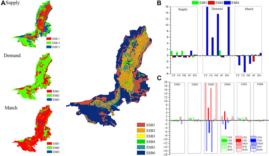
FIGURE 6. Spatial distribution of ES bundles for supply, demand, match degree, and all three ES components (A), and z-score values of ESs in each bundle (B) and (C).

3.3 Driving Mechanisms of ES Supply, Demand, and Match Degree

Twenty possible socioecological factors were selected to analyze the driving mechanisms of ES distribution and interactions. Using random forest analysis, we tried to identify the most critical factors of ES supply, demand, and match degree by comparing their relative impacts and explained variance for ES distribution. Then, 14 factors were selected, including dem, prec, wind, soil, discity, discrop, disgrass, disurban, disroad, GDPden, perGDP, NDVI, land use, and urbanland (Table 6).

TABLE 6

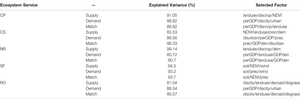
TABLE 6. Selected socioecological factors for ES supply, demand, and match degree and their explained variances.

To explore the socioecological background of the ES bundles, these 14 factors were clustered using the SOM clustering method and then overlaid with the ES bundles (Figure 7). The results suggest that the study area could be divided into six different clusters according to the spatial pattern of these socioecological factors. Driver cluster 1 (DC 1) was in the southern part of the CBYN with the highest distance to artificial and semiartificial facilities, such as city centers, cropland, and transportation. DC 2 was distributed in the southern and northern mountains with the highest elevation and the second-largest distance to artificial and semiartificial facilities. DC 3 and DC 4 were both distributed in the central plain with lower elevation and were closer to city centers, cropland, and urban areas but far away from grassland; DC 3 was concentrated in urban and rural areas with the highest per GDP, and DC 4 was in cropland with the highest NDVI values. DC 5 and DC 6 were both distributed in the transition region between the central plain and the fringe mountains; the former was in the northern part with the highest precipitation and moderate GDP density, and the latter was in the southern part with the lowest precipitation and lowest GDP density. As indicated by the results of the overlay analysis (Figure 7B), ESB 3 and ESB 4 mostly overlapped with DC 3, while ESB 2 and ESB 5 had a higher overlap percentage with DC 4 and DC 6. ESB 1 mainly overlapped with DC 5 (66.248%) and overlapped little with DC 6 (15.301%) and DC 2 (10.844%), while ESB 6 overlapped with DC 5 (82.799%), DC 2 (30.395%), and DC 6 (19.992%). Overall, ES supply–demand characteristics can be predicted by the socioecological environment to some extent, while different socioecological environments generate the same ES supply–demand characteristics.

FIGURE 7

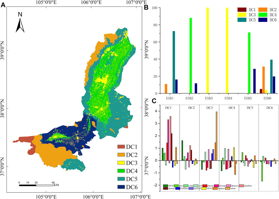
FIGURE 7. Spatial distribution of driver clusters (A), overlap percentage of driver clusters and ES bundles (B), and z-score values of each driver in different clusters (C).

3.4 Ecosystem Zoning Management and Measures

To maintain the sustainable supply of multiple ESs, the socioecological system must be managed in a manner that can balance ES supply and demand. By combining the characteristics of ES supply and demand, their tradeoffs and bundles, and the socioecological environment, zoning management was conducted, as shown in Figure 8. According to the characteristics of different zones, combining the driving mechanism of each ES, zoning management measures were proposed, as shown in Table 7 below.

FIGURE 8

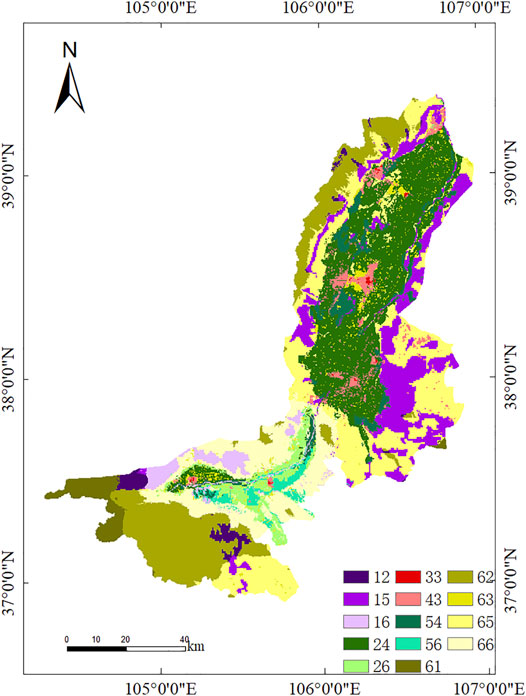
FIGURE 8. Zoning management in the CBYN.

TABLE 7

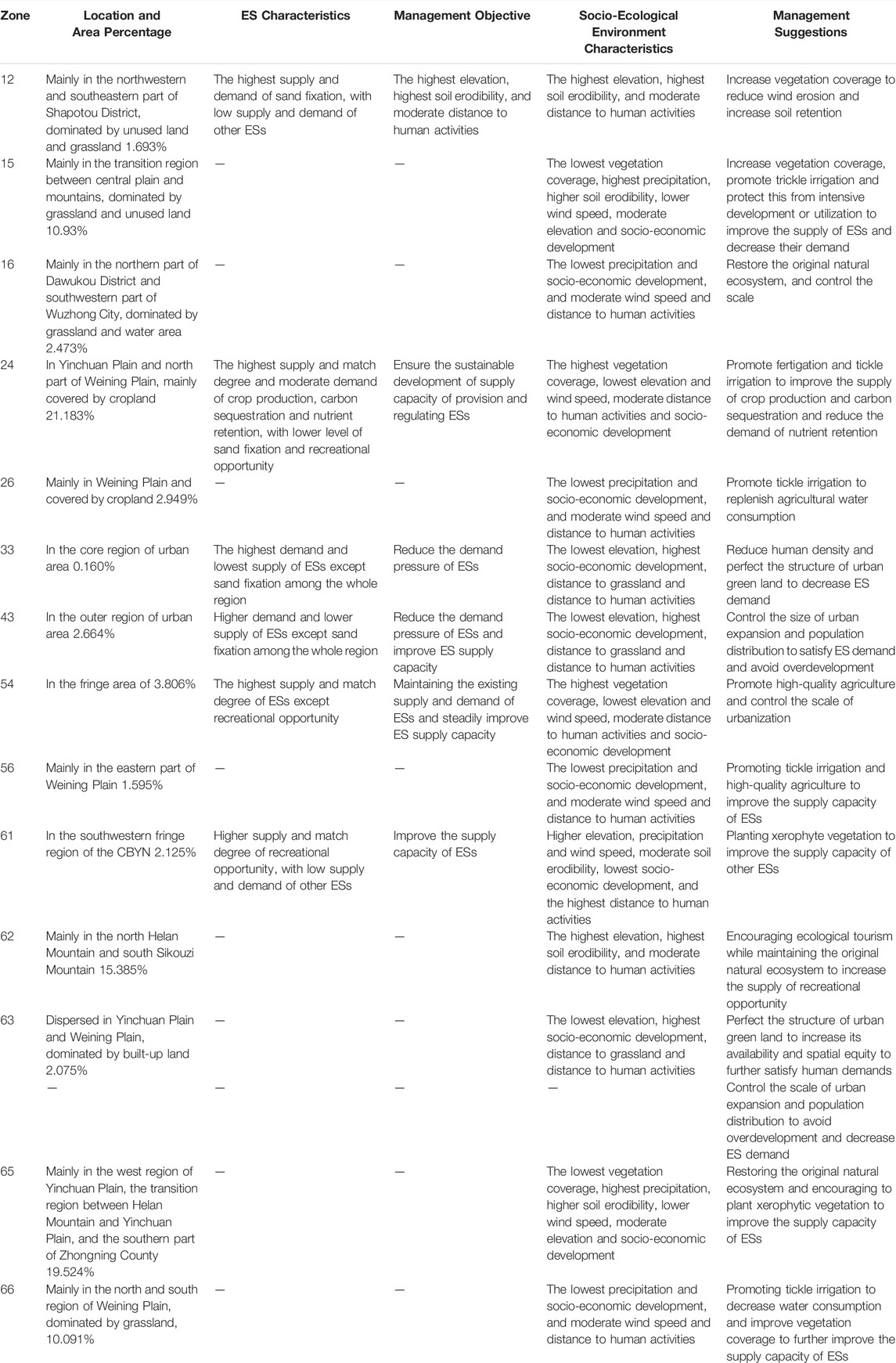
TABLE 7. Ecosystem zoning management measures.

4 Discussion

4.1 Spatial Mismatches of ES Supply and Demand

In the CBYN, high supply and low demand of ESs exist in croplands with high human utilization in the central plain, with low supply and high demand in grassland with a more natural environment. This is inconsistent with the findings in the European, which suggested that hotspots of ES supply exist in more natural mountain regions, with high demand in urbanized areas or intensive agricultural areas in the lowlands (Schirpke et al., 2019). This can be explained by the characteristics of the study area. Low precipitation in arid and semiarid regions limits vegetation coverage and growth (Georganos et al., 2017), resulting in large areas of sparse grassland and even bare land or deserts, which have low supply and low demand of ESs. Thus, the natural environment does not equate to hotspots of ES supply, or the low supply and demand of ESs, especially in arid and semiarid regions.

Land use patterns directly impact the configuration and magnitude of ESs and further affect the sustainability and resilience of the ecosystem (Marques et al., 2019; Zhou et al., 2021). They play a critical role in determining the spatial pattern of ES supply, which is consistent with the findings in other studies (Meacham et al., 2016; Spake et al., 2017; Xu et al., 2018), but cannot explain all the variance. For ES supply, cropland distribution and vegetation coverage have the second largest impacts, suggesting the ecological importance of cropland management in the CBYN. The Yellow River goes through the CBYN, providing abundant water resources for agricultural production and for sustaining the cropland with a high and intensive vegetation cover. The management of the cropland is critical for future sustainable development, especially in the Yellow River basin. Mountain areas with forest coverage and steep terrains could provide a high supply of regulating and cultural services, i.e., carbon sequestration, sand fixation, and recreational opportunity, especially in arid and semiarid regions (Fu et al., 2017). Moreover, this area also has a high supply of wind prevention and sand fixation, which has great importance in building good living conditions for human settlement in the central plain (Lyu et al., 2018). The exclusion of human intervention also makes the mountain areas a low-demand area for ESs. Therefore, even in arid and semiarid regions, the mountains remain ecological hotspots with strong positive spillover effects (Wei et al., 2018; Chen et al., 2019).

Lorilla et al. (2019) suggested that excess ES demand can inhibit the supply of other ESs. In our study, high demand and low supply of ESs existed in the urban areas, especially in the city center with the densest settlement. Thus, the compact city, which has been widely promoted in urban planning due to its advantages in social cohesion and land efficiency, would have negative impacts on ES conservation, especially for provision and regulating services. This is consistent with the “paradox of the compact city” in Berlin (Larondelle and Lauf, 2016). Green spaces in urban areas would be a solution to tackle this paradox and turn it into a win–win situation, as indicated by the higher supply and lower demand of ESs in the outer city (Guan et al., 2020). Dense settlement in the city center is closely correlated with high imperviousness of the land surface, which has been suggested as a critical driver for the low ES supply in urban areas (Zhang et al., 2017; Tao et al., 2018). Minimizing the paved area in settlements would be helpful in the sustainable planning of city centers. On the other hand, urban land also has a high supply and high match degree for cultural services, especially in the outer city. This also is another promising future for urban development, i.e., utilizing tourism resources and building scenic spots.

4.2 Tradeoffs and Synergies Among ESs

Tradeoffs/synergies among ESs mainly come from two resources. The first is ESs intrinsically correlated with the same ecological process or those that benefit stakeholders, e.g., the photosynthesis process in vegetation growth would increase the carbon sequestration service but decrease water resources, resulting in the tradeoff between carbon sequestration and water yield (Zhou et al., 2017); crop production and recreational opportunity both aim to satisfy the demand of the same stakeholders (Stålhammar and Pedersen, 2017; Ala-Hulkko et al., 2019). The second is ESs externally impacted by the same socioecological factors, e.g., high elevation is beneficial for wind prevention and sand fixation but harmful for crop production, contributing to their tradeoff (Shi et al., 2009; Li and Wang, 2018). In our study, synergies among crop production, carbon sequestration, and nutrient retention in supply may be caused by their close correlation with vegetation growth. In specific, crop production and nutrient retention have a closer relation to crop growth in the central plain, while carbon sequestration is also impacted by forest growth, as indicated by the hotspots in the mountain areas and the high impacts of precipitation and elevation. These factors finally result in a stronger synergy between food production and nutrient retention and a weaker one between carbon sequestration and the other two services. Overall, the closer to the same ecological process or the same stakeholders, the stronger the relationship between the two ESs.

Recreational opportunity supply and sand fixation had greater differences from the other three ESs in the related ecological process and estimation method, while they only had similarities in their driving mechanisms to a certain extent, with the common influencing factors of land use pattern and NDVI. The lack of intrinsic correlation and low similarity of the external driving mechanisms finally result in a weak correlation between the former two ESs and the other three ESs on the supply side, which is consistent with the findings in relevant studies (Obiang Ndong et al., 2020; Lyu et al., 2021). The same situation occurs at the match and demand sides. The unstable tradeoffs or synergies among ESs mainly result from the lack of intrinsic relations or similar calculation methods among ESs at the match side, as ES demand comes from the recalculation of ES supply and demand. In our study, the ES demand was calculated with significant differences: two from the requirements of human beings (crop production and recreational opportunity), two from pollutants emitted in the ecosystem (carbon sequestration and nutrient retention), and one from an ecological process (sand fixation). Among them, stronger relationships exist among ESs in the same group at the demand side, while weaker relationships exist among ESs in different groups. Cui et al. (2019) also suggested the same conclusion. Overall, the synergies and tradeoffs among ESs can be partly predicted based on the similarity of calculation methods and intrinsic ecological processes. Moreover, per capita GDP, a good comprehensive indicator for economic development and population growth, has the most critical impact on the four ESs on the demand side except for sand fixation, which contributes to the stronger synergies among ES demands at the county scale. This should be taken into consideration in land use policy-making.

4.3 Integrating ES Supply–Demand and the Socioecological System Into Ecosystem Zoning Management

Significant spatial heterogeneities exist in different zones, including key environmental issues, social conditions, and ecological environment, which calls for differentiated, targeted management policies (Ai et al., 2015; Li et al., 2021). Zoning management can satisfy this need at multiple scales for different protection targets (Dubrova et al., 2015). For example, the U.S. Environmental Protection Agency developed a water ecological zoning in the mid-1980s at the national scale, which has been successfully applied to protect the entire hydroecological system and water quality (Xu et al., 2020). In China, the Ecological Red Line system has been launched to classify strict protection areas with special and critical ecological functions to maintain national ecological security. However, the delineation of the Ecological Protection Red Line has conflicted with the boundary of Permanent Basic Arable land and the need for economic development (He et al., 2018). A more rational zoning management method is desired at the local scale.

This study presented an integrated framework to integrate ESs and the socioecological environment in zoning management, including mapping the supply and demand of multiple ESs, assessing interactions among ESs, quantifying their socioecological mechanisms, and finally overlaying ES bundles and socioecological driver clusters to classify zones and provide management suggestions. By considering both the supply and demand sides of multiple ESs in the framework, we can identify the ecological problems from the comprehensive insights of natural, ecological, social, and economic systems, which is beneficial for balancing environmental protection and socioeconomic development (Peng et al., 2019a). Through quantifying the socioecological driving mechanisms of ESs, differentiated management strategies have been designed for different zones to adapt to local conditions. The strategy of one-size-fits-all is unsuitable for land use planning and ecosystem management (Zhou et al., 2019).

Numerous studies have focused on avoiding irrational human activities and protecting natural capital (Bradford and D'Amato, 2012; Cai et al., 2017; Fernandino et al., 2018). The urgent challenge is integrating research results into actual actions through social policy and decision-making (Gong et al., 2021). Based on the analysis results of ES bundles and socioecological driver clusters, the CBYN can be divided into 14 zones with different ES supply–demand characteristics, ES tradeoffs/synergies, and socioecological conditions. Differentiated management strategies have been suggested for different zones to enhance the ES supply–demand match degrees and synergies among ESs and reduce tradeoffs (Table 7).

4.4 Limitations and Directions

In this study, the key ESs were selected by considering not only the natural environment but also human well-being, while their supply and demand were quantified and mapped through widely accepted models and equations. Data in this study were readily obtained, including remote sensing images, meteorological observations, and social statistics. As for the approach to identifying ecological problems and management objectives, spatial neighborhood impacts were taken into consideration rather than directly overlaying multiple ESs. This approach could contribute to identifying spatially aggregated multiple ESs rather than isolated grids with high or low values of ESs through the SOM method. Besides that, Spearman’s rank correlation analysis has been confronted as a simple but effective method for analyzing correlations among ESs. However, there are still some limitations.

First, tradeoffs/synergies among ESs are scale-dependent, that is, they are likely to change with the spatial unit. The results of ES interactions might only be applicable at a specific temporal or spatial scale in the study (Peng et al., 2019a). Future research would focus on comparative analysis at multiple scales. Second, this study did not include institutional and cultural factors in building a socioecological driver system, which has important impacts on socioeconomic development and human demands, especially in China. Future studies should focus more on finer and deeper identification of key drivers of ES tradeoffs/synergies, such as the impacts of management practices, landscape patterns, and soil characteristics.

5 Conclusion

This study established a framework for systematically proposing a zoning management method by exploring the spatial relationships among ESs and their driving mechanisms at both supply and demand sides. The results suggest that significant differences exist in ES spatial distribution at different sides of supply, demand, and match degree. High values of ES supply were mainly concentrated in the central plain, which was mostly impacted by land use patterns, cropland distribution, and vegetation coverage. Meanwhile, high ES demand was mainly concentrated in urban areas, especially the city center, which was mainly driven by per capita GDP. Spatial interactions among ESs varied greatly among the three sides of supply, demand, and match degree, especially between the two ESs of sand fixation and recreational opportunity and the other three ESs. Significant synergies existed among crop production, carbon sequestration, and nutrient retention, which kept consistent at different sides of supply and demand. This was caused by the similarities in their intrinsic ecological processes and beneficiaries. On the other hand, the lack of intrinsic correlation and low similarity of the external driving mechanisms resulted in weak and unstable interactions between the two ESs of sand fixation and recreational opportunity and the other three ESs at different sides. Overlay analysis of ES bundles and driver clusters is a useful way to identify management zones with relatively consistent ecological problems and socioecological environments, and differentiated management suggestions were provided to sustain the supply–demand match degree of multiple ESs simultaneously.

Data Availability Statement

The original contributions presented in the study are included in the article/Supplementary Material; further inquiries can be directed to the corresponding author.

Author Contributions

RL: conceptualization, data curation, methodology, formal analysis, writing, project administration; XT: methodology, resources, software; WZ: supervision, validation, visualization; JP: data analysis, visualization; JZ: funding acquisition, investigation, supervision.

Funding

This study was supported by the National Natural Science Foundation of China (Grant No. 42101288 and 42071290).

Conflict of Interest

The authors declare that the research was conducted in the absence of any commercial or financial relationships that could be construed as a potential conflict of interest.

Publisher’s Note

All claims expressed in this article are solely those of the authors and do not necessarily represent those of their affiliated organizations, or those of the publisher, the editors, and the reviewers. Any product that may be evaluated in this article, or claim that may be made by its manufacturer, is not guaranteed or endorsed by the publisher.

Supplementary Material

The Supplementary Material for this article can be found online at: https://www.frontiersin.org/articles/10.3389/fenvs.2022.911190/full#supplementary-material

References

Ai, J., Sun, X., Feng, L., Li, Y., and Zhu, X. (2015). Analyzing the Spatial Patterns and Drivers of Ecosystem Services in Rapidly Urbanizing Taihu Lake Basin of China. Front. Earth Sci. 9, 531–545. doi:10.1007/s11707-014-0484-1

CrossRef Full Text | Google Scholar

Ala-Hulkko, T., Kotavaara, O., Alahuhta, J., and Hjort, J. (2019). Mapping Supply and Demand of a Provisioning Ecosystem Service across Europe. Ecol. Indic. 103, 520–529. doi:10.1016/j.ecolind.2019.04.049

CrossRef Full Text | Google Scholar

Bagstad, K. J., Johnson, G. W., Voigt, B., and Villa, F. (2013). Spatial Dynamics of Ecosystem Service Flows: A Comprehensive Approach to Quantifying Actual Services. Ecosyst. Serv. 4, 117–125. doi:10.1016/j.ecoser.2012.07.012

CrossRef Full Text | Google Scholar

Birgé, H. E., Allen, C. R., Garmestani, A. S., and Pope, K. L. (2016). Adaptive Management for Ecosystem Services. J. Environ. Manag. 183, 343–352. doi:10.1016/j.jenvman.2016.07.054

CrossRef Full Text | Google Scholar

Bradford, J. B., and D'Amato, A. W. (2012). Recognizing Trade-Offs in Multi-Objective Land Management. Front. Ecol. Environ. 10, 210–216. doi:10.1890/110031

CrossRef Full Text | Google Scholar

Cai, W., Gibbs, D., Zhang, L., Ferrier, G., and Cai, Y. (2017). Identifying Hotspots and Management of Critical Ecosystem Services in Rapidly Urbanizing Yangtze River Delta Region, China. J. Environ. Manag. 191, 258–267. doi:10.1016/j.jenvman.2017.01.003

CrossRef Full Text | Google Scholar

Chang, C.-T., Song, C.-E., Lee, L.-C., Chan, S.-C., Liao, C.-S., Liou, Y.-S., et al. (2021). Influence of Landscape Mosaic Structure on Nitrate and Phosphate Discharges: An Island-wide Assessment in Subtropical Mountainous Taiwan. Landsc. Urban Plan. 207, 104017. doi:10.1016/j.landurbplan.2020.104017

CrossRef Full Text | Google Scholar

Chen, T., Feng, Z., Zhao, H., and Wu, K. (2019). Identification of Ecosystem Service Bundles and Driving Factors in Beijing and its Surrounding Areas. Sci. Total Environ. 711, 134687. doi:10.1016/j.scitotenv.2019.134687

PubMed Abstract | CrossRef Full Text | Google Scholar

Cord, A. F., Bartkowski, B., Beckmann, M., Dittrich, A., Hermans-Neumann, K., Kaim, A., et al. (2017). Towards Systematic Analyses of Ecosystem Service Trade-Offs and Synergies: Main Concepts, Methods and the Road Ahead. Ecosyst. Serv. 28, 264–272. doi:10.1016/j.ecoser.2017.07.012

CrossRef Full Text | Google Scholar

Costanza, R., d'Arge, R., de Groot, R., Farber, S., Grasso, M., Hannon, B., et al. (1997). The Value of the World's Ecosystem Services and Natural Capital. Nature 387, 253–260. doi:10.1038/387253a0

CrossRef Full Text | Google Scholar

Cui, F., Tang, H., Zhang, Q., Wang, B., and Dai, L. (2019). Integrating Ecosystem Services Supply and Demand into Optimized Management at Different Scales: A Case Study in Hulunbuir, China. Ecosyst. Serv. 39, 100984. doi:10.1016/j.ecoser.2019.100984

CrossRef Full Text | Google Scholar

Dong, L., and Ma, J. (2012). Existing Problems in the Urban Landscaping and Greening Management in Yinchuan City and the Coping Strategies. Anhui For. Sci. Technol. 38, 61–63.

Google Scholar

Dubrova, S. V., Podlipskiy, I. I., Kurilenko, V. V., and Siabato, W. (2015). Functional City Zoning. Environmental Assessment of Eco-Geological Substance Migration Flows. Environ. Pollut. 197, 165–172. doi:10.1016/j.envpol.2014.12.013

PubMed Abstract | CrossRef Full Text | Google Scholar

Fernandino, G., Elliff, C. I., and Silva, I. R. (2018). Ecosystem-based Management of Coastal Zones in Face of Climate Change Impacts: Challenges and Inequalities. J. Environ. Manag. 215, 32–39. doi:10.1016/j.jenvman.2018.03.034

CrossRef Full Text | Google Scholar

Fu, Q., Li, B., Hou, Y., Bi, X., and Zhang, X. (2017). Effects of Land Use and Climate Change on Ecosystem Services in Central Asia's Arid Regions: A Case Study in Altay Prefecture, China. Sci. Total Environ. 607-608, 633–646. doi:10.1016/j.scitotenv.2017.06.241

PubMed Abstract | CrossRef Full Text | Google Scholar

Furst, C., Frank, S., Witt, A., Koschke, L., and Makeschin, F. (2013). Assessment of the Effects of Forest Land Use Strategies on the Provision of Ecosystem Services at Regional Scale. J. Environ. Manag. 127 (Suppl. l), S96–S116. doi:10.1016/j.jenvman.2012.09.020

CrossRef Full Text | Google Scholar

Georganos, S., Abdi, A. M., Tenenbaum, D. E., and Kalogirou, S. (2017). Examining the NDVI-Rainfall Relationship in the Semi-arid Sahel Using Geographically Weighted Regression. J. Arid Environ. 146, 64–74. doi:10.1016/j.jaridenv.2017.06.004

CrossRef Full Text | Google Scholar

Gong, J., Cao, E., Xie, Y., Xu, C., Li, H., and Yan, L. (2021). Integrating Ecosystem Services and Landscape Ecological Risk into Adaptive Management: Insights from a Western Mountain-Basin Area, China. J. Environ. Manag. 281, 111817. doi:10.1016/j.jenvman.2020.111817

CrossRef Full Text | Google Scholar

Guan, D., He, X., He, C., Cheng, L., and Qu, S. (2020). Does the Urban Sprawl Matter in Yangtze River Economic Belt, China? an Integrated Analysis with Urban Sprawl Index and One Scenario Analysis Model. Cities 99, 102611. doi:10.1016/j.cities.2020.102611

CrossRef Full Text | Google Scholar

Hauck, J., Winkler, K. J., and Priess, J. A. (2015). Reviewing Drivers of Ecosystem Change as Input for Environmental and Ecosystem Services Modelling. Sustain. Water Qual. Ecol. 5, 9–30. doi:10.1016/j.swaqe.2015.01.003

CrossRef Full Text | Google Scholar

He, P., Gao, J., Zhang, W., Rao, S., Zou, C., Du, J., et al. (2018). China Integrating Conservation Areas into Red Lines for Stricter and Unified Management. Land Use Policy 71, 245–248. doi:10.1016/j.landusepol.2017.11.057

CrossRef Full Text | Google Scholar

Hu, Y. n., Peng, J., Liu, Y., and Tian, L. (2018). Integrating Ecosystem Services Trade-Offs with Paddy Land-To-Dry Land Decisions: A Scenario Approach in Erhai Lake Basin, Southwest China. Sci. Total Environ. 625, 849–860. doi:10.1016/j.scitotenv.2017.12.340

PubMed Abstract | CrossRef Full Text | Google Scholar

Huang, Q., Yin, D., He, C., Yan, J., Liu, Z., Meng, S., et al. (2020). Linking Ecosystem Services and Subjective Well-Being in Rapidly Urbanizing Watersheds: Insights from a Multilevel Linear Model. Ecosyst. Serv. 43, 101106. doi:10.1016/j.ecoser.2020.101106

CrossRef Full Text | Google Scholar

Ito, A., Nishina, K., and Noda, H. M. (2016). Evaluation of Global Warming Impacts on the Carbon Budget of Terrestrial Ecosystems in Monsoon Asia: a Multi-Model Analysis. Ecol. Res. 31, 459–474. doi:10.1007/s11284-016-1354-y

CrossRef Full Text | Google Scholar

Jiang, C., Li, D., Wang, D., and Zhang, L. (2016). Quantification and Assessment of Changes in Ecosystem Service in the Three-River Headwaters Region, China as a Result of Climate Variability and Land Cover Change. Ecol. Indic. 66, 199–211. doi:10.1016/j.ecolind.2016.01.051

CrossRef Full Text | Google Scholar

Larondelle, N., and Lauf, S. (2016). Balancing Demand and Supply of Multiple Urban Ecosystem Services on Different Spatial Scales. Ecosyst. Serv. 22, 18–31. doi:10.1016/j.ecoser.2016.09.008

CrossRef Full Text | Google Scholar

Li, B., and Wang, W. (2018). Trade-offs and Synergies in Ecosystem Services for the Yinchuan Basin in China. Ecol. Indic. 84, 837–846. doi:10.1016/j.ecolind.2017.10.001

CrossRef Full Text | Google Scholar

Li, H., Qiu, J., Wang, L., Tang, H., Li, C., and Van Ranst, E. (2010). Modelling Impacts of Alternative Farming Management Practices on Greenhouse Gas Emissions from a Winter Wheat–Maize Rotation System in China. Agric. Ecosyst. Environ. 135, 24–33. doi:10.1016/j.agee.2009.08.003

CrossRef Full Text | Google Scholar

Li, R., Lin, H., Niu, H., Chen, Y., Zhao, S., and Fan, L. (2017). Effects of Irrigation on the Ecological Services in an Intensive Agricultural Region in China: A Trade-Off Perspective. J. Clean. Prod. 156, 41–49. doi:10.1016/j.jclepro.2017.04.031

CrossRef Full Text | Google Scholar

Li, X., Yu, X., Wu, K., Feng, Z., Liu, Y., and Li, X. (2021). Land-use Zoning Management to Protecting the Regional Key Ecosystem Services: A Case Study in the City Belt along the Chaobai River, China. Sci. Total Environ. 762, 143167. doi:10.1016/j.scitotenv.2020.143167

PubMed Abstract | CrossRef Full Text | Google Scholar

Lorilla, R. S., Kalogirou, S., Poirazidis, K., and Kefalas, G. (2019). Identifying Spatial Mismatches between the Supply and Demand of Ecosystem Services to Achieve a Sustainable Management Regime in the Ionian Islands (Western Greece). Land Use Policy 88, 104171. doi:10.1016/j.landusepol.2019.104171

CrossRef Full Text | Google Scholar

Lyu, R., Zhang, J., Xu, M., and Li, J. (2018). Impacts of Urbanization on Ecosystem Services and Their Temporal Relations: A Case Study in Northern Ningxia, China. Land Use Policy 77, 163–173. doi:10.1016/j.landusepol.2018.05.022

CrossRef Full Text | Google Scholar

Lyu, R., Clarke, K. C., Zhang, J., Feng, J., Jia, X., and Li, J. (2019). Spatial Correlations Among Ecosystem Services and Their Socio-Ecological Driving Factors: A Case Study in the City Belt along the Yellow River in Ningxia, China. Appl. Geogr. 108, 64–73. doi:10.1016/j.apgeog.2019.05.003

CrossRef Full Text | Google Scholar

Lyu, R., Clarke, K. C., Zhang, J., Feng, J., Jia, X., and Li, J. (2021). Dynamics of Spatial Relationships Among Ecosystem Services and Their Determinants: Implications for Land Use System Reform in Northwestern China. Land Use Policy 102, 105231. doi:10.1016/j.landusepol.2020.105231

CrossRef Full Text | Google Scholar

Marques, A., Martins, I. S., Kastner, T., Plutzar, C., Theurl, M. C., Eisenmenger, N., et al. (2019). Increasing Impacts of Land Use on Biodiversity and Carbon Sequestration Driven by Population and Economic Growth. Nat. Ecol. Evol. 3, 628–637. doi:10.1038/s41559-019-0824-3

PubMed Abstract | CrossRef Full Text | Google Scholar

MEA (2005). Ecosystems and Human Well-Being: Scenarios: Findings of the Scenarios Working Group. Washington DC: Island Press.

Google Scholar

Meacham, M., Queiroz, C., Norström, A. V., and Peterson, G. D. (2016). Social-ecological Drivers of Multiple Ecosystem Services: what Variables Explain Patterns of Ecosystem Services across the Norrström Drainage Basin? Ecol. Soc. 21 (1), 14. doi:10.5751/es-08077-210114

CrossRef Full Text | Google Scholar

Meng, S., Huang, Q., Zhang, L., He, C., Inostroza, L., Bai, Y., et al. (2020). Matches and Mismatches between the Supply of and Demand for Cultural Ecosystem Services in Rapidly Urbanizing Watersheds: A Case Study in the Guanting Reservoir Basin, China. Ecosyst. Serv. 45, 101156. doi:10.1016/j.ecoser.2020.101156

CrossRef Full Text | Google Scholar

Mouchet, M. A., Paracchini, M. L., Schulp, C. J. E., Stürck, J., Verkerk, P. J., Verburg, P. H., et al. (2017). Bundles of Ecosystem (Dis)services and Multifunctionality across European Landscapes. Ecol. Indic. 73, 23–28. doi:10.1016/j.ecolind.2016.09.026

CrossRef Full Text | Google Scholar

Nahuelhual, L., Vergara, X., Kusch, A., Campos, G., and Droguett, D. (2017). Mapping Ecosystem Services for Marine Spatial Planning: Recreation Opportunities in Sub-antarctic Chile. Mar. Policy 81, 211–218. doi:10.1016/j.marpol.2017.03.038

CrossRef Full Text | Google Scholar

Obiang Ndong, G., Therond, O., and Cousin, I. (2020). Analysis of Relationships between Ecosystem Services: A Generic Classification and Review of the Literature. Ecosyst. Serv. 43, 101120. doi:10.1016/j.ecoser.2020.101120

CrossRef Full Text | Google Scholar

Peng, J., Hu, X., Qiu, S., Hu, Y. n., Meersmans, J., and Liu, Y. (2019a). Multifunctional Landscapes Identification and Associated Development Zoning in Mountainous Area. Sci. Total Environ. 660, 765–775. doi:10.1016/j.scitotenv.2019.01.023

PubMed Abstract | CrossRef Full Text | Google Scholar

Peng, J., Hu, X., Wang, X., Meersmans, J., Liu, Y., and Qiu, S. (2019b). Simulating the Impact of Grain-For-Green Programme on Ecosystem Services Trade-Offs in Northwestern Yunnan, China. Ecosyst. Serv. 39, 100998. doi:10.1016/j.ecoser.2019.100998

CrossRef Full Text | Google Scholar

Qi, W., Liu, S., Gao, X., and Zhao, M. (2015). Modeling the Spatial Distribution of Urban Population during the Daytime and at Night Based on Land Use: A Case Study in Beijing, China. J. Geogr. Sci. 25, 756–768. doi:10.1007/s11442-015-1200-0

CrossRef Full Text | Google Scholar

Raudsepp-Hearne, C., Peterson, G. D., and Bennett, E. M. (2010). Ecosystem Service Bundles for Analyzing Tradeoffs in Diverse Landscapes. Proc. Natl. Acad. Sci. U.S.A. 107, 5242–5247. doi:10.1073/pnas.0907284107

PubMed Abstract | CrossRef Full Text | Google Scholar

Redhead, J. W., May, L., Oliver, T. H., Hamel, P., Sharp, R., and Bullock, J. M. (2018). National Scale Evaluation of the InVEST Nutrient Retention Model in the United Kingdom. Sci. Total Environ. 610-611, 666–677. doi:10.1016/j.scitotenv.2017.08.092

PubMed Abstract | CrossRef Full Text | Google Scholar

Schirpke, U., Candiago, S., Egarter Vigl, L., Jäger, H., Labadini, A., Marsoner, T., et al. (2019). Integrating Supply, Flow and Demand to Enhance the Understanding of Interactions Among Multiple Ecosystem Services. Sci. Total Environ. 651, 928–941. doi:10.1016/j.scitotenv.2018.09.235

PubMed Abstract | CrossRef Full Text | Google Scholar

Shi, N., Zhan, J., Wu, F., and Du, J. (2009). Identification of the Core Ecosystem Services and Their Spatial Heterogeneity in Poyang Lake Area. Front. Earth Sci. China 3, 214–220. doi:10.1007/s11707-009-0008-6

CrossRef Full Text | Google Scholar

Spake, R., Lasseur, R., Crouzat, E., Bullock, J. M., Lavorel, S., Parks, K. E., et al. (2017). Unpacking Ecosystem Service Bundles: Towards Predictive Mapping of Synergies and Trade-Offs between Ecosystem Services. Glob. Environ. Change 47, 37–50. doi:10.1016/j.gloenvcha.2017.08.004

CrossRef Full Text | Google Scholar

Stålhammar, S., and Pedersen, E. (2017). Recreational Cultural Ecosystem Services: How Do People Describe the Value? Ecosyst. Serv. 26, 1–9. doi:10.1016/j.ecoser.2017.05.010

CrossRef Full Text | Google Scholar

Stevens, F. R., Gaughan, A. E., Linard, C., and Tatem, A. J. (2015). Disaggregating Census Data for Population Mapping Using Random Forests with Remotely-Sensed and Ancillary Data. PLoS One 10, e0107042. doi:10.1371/journal.pone.0107042

PubMed Abstract | CrossRef Full Text | Google Scholar

Su, K., Sun, X., Guo, H., Long, Q., Li, S., Mao, X., et al. (2020). The Establishment of a Cross-Regional Differentiated Ecological Compensation Scheme Based on the Benefit Areas and Benefit Levels of Sand-Stabilization Ecosystem Service. J. Clean. Prod. 270, 122490. doi:10.1016/j.jclepro.2020.122490

CrossRef Full Text | Google Scholar

Sun, W., Li, D., Wang, X., Li, R., Li, K., and Xie, Y. (2019). Exploring the Scale Effects, Trade-Offs and Driving Forces of the Mismatch of Ecosystem Services. Ecol. Indic. 103, 617–629. doi:10.1016/j.ecolind.2019.04.062

CrossRef Full Text | Google Scholar

Tan, M., Liu, K., Liu, L., Zhu, Y., and Wang, D. (2017). Spatialization of Population in the Pearl River Delta in 30 M Grids Using Random Forest Model. Prog. Geogr. 36, 1304–1312. doi:10.18306/dlkxjz.2017.10.012

CrossRef Full Text | Google Scholar

Tao, Y., Wang, H., Ou, W., and Guo, J. (2018). A Land-Cover-Based Approach to Assessing Ecosystem Services Supply and Demand Dynamics in the Rapidly Urbanizing Yangtze River Delta Region. Land Use Policy 72, 250–258. doi:10.1016/j.landusepol.2017.12.051

CrossRef Full Text | Google Scholar

Wang, B., Gao, P., Niu, X., and Sun, J. (2017). Policy-driven China’s Grain to Green Program: Implications for Ecosystem Services. Ecosyst. Serv. 27, 38–47. doi:10.1016/j.ecoser.2017.07.014

CrossRef Full Text | Google Scholar

Wei, H., Fan, W., Wang, X., Lu, N., Dong, X., Zhao, Y., et al. (2017). Integrating Supply and Social Demand in Ecosystem Services Assessment: A Review. Ecosyst. Serv. 25, 15–27. doi:10.1016/j.ecoser.2017.03.017

CrossRef Full Text | Google Scholar

Wei, H., Liu, H., Xu, Z., Ren, J., Lu, N., Fan, W., et al. (2018). Linking Ecosystem Services Supply, Social Demand and Human Well-Being in a Typical Mountain–Oasis–Desert Area, Xinjiang, China. Ecosyst. Serv. 31, 44–57. doi:10.1016/j.ecoser.2018.03.012

CrossRef Full Text | Google Scholar

Xu, S., Liu, Y., Wang, X., and Zhang, G. (2017). Scale Effect on Spatial Patterns of Ecosystem Services and Associations Among Them in Semi-arid Area: A Case Study in Ningxia Hui Autonomous Region, China. Sci. Total Environ. 598, 297–306. doi:10.1016/j.scitotenv.2017.04.009

PubMed Abstract | CrossRef Full Text | Google Scholar

Xu, X., Yang, G., Tan, Y., Liu, J., and Hu, H. (2018). Ecosystem Services Trade-Offs and Determinants in China's Yangtze River Economic Belt from 2000 to 2015. Sci. Total Environ. 634, 1601–1614. doi:10.1016/j.scitotenv.2018.04.046

PubMed Abstract | CrossRef Full Text | Google Scholar

Xu, J., Xiao, Y., Xie, G., Wang, Y., and Jiang, Y. (2019a). Computing Payments for Wind Erosion Prevention Service Incorporating Ecosystem Services Flow and Regional Disparity in Yanchi County. Sci. Total Environ. 674, 563–579. doi:10.1016/j.scitotenv.2019.03.361

PubMed Abstract | CrossRef Full Text | Google Scholar

Xu, L.-X., Yang, D.-W., Wu, T.-H., Yi, S.-H., Fang, Y.-P., Xiao, C.-D., et al. (2019b). An Ecosystem Services Zoning Framework for the Permafrost Regions of China. Adv. Clim. Change Res. 10, 92–98. doi:10.1016/j.accre.2019.06.007

CrossRef Full Text | Google Scholar

Xu, K., Wang, J., Wang, J., Wang, X., Chi, Y., and Zhang, X. (2020). Environmental Function Zoning for Spatially Differentiated Environmental Policies in China. J. Environ. Manag. 255, 109485. doi:10.1016/j.jenvman.2019.109485

CrossRef Full Text | Google Scholar

Yang, Y., Feng, Y., Yang, S., Cao, Y., Liu, Q., and Yang, G. (2011). Economic Loss Caused by Non-point Source Pollution-A Case Study of Ningxia Yellow River Water Irrigation District. Agric. Res. Arid Areas 29, 242–246.

Google Scholar

Yu, Y., Li, J., Zhou, Z., Ma, X., and Zhang, X. (2021). Response of Multiple Mountain Ecosystem Services on Environmental Gradients: How to Respond, and where Should Be Priority Conservation? J. Clean. Prod. 278, 123264. doi:10.1016/j.jclepro.2020.123264

CrossRef Full Text | Google Scholar

Zeng, L., Li, J., Zhou, Z., and Yu, Y. (2020). Optimizing Land Use Patterns for the Grain for Green Project Based on the Efficiency of Ecosystem Services under Different Objectives. Ecol. Indic. 114, 106347. doi:10.1016/j.ecolind.2020.106347

CrossRef Full Text | Google Scholar

Zhang, W., Huang, B., and Luo, D. (2014). Effects of Land Use and Transportation on Carbon Sources and Carbon Sinks: A Case Study in Shenzhen, China. Landsc. Urban Plan. 122, 175–185. doi:10.1016/j.landurbplan.2013.09.014

CrossRef Full Text | Google Scholar

Zhang, H., Wang, Q., Li, G., Zhang, H., and Zhang, J. (2017). Losses of Ecosystem Service Values in the Taihu Lake Basin from 1979 to 2010. Front. Earth Sci. 11, 310–320. doi:10.1007/s11707-016-0612-1

CrossRef Full Text | Google Scholar

Zhou, L., and Yan, X. (2009). Eco-Tourism System and its Sustainable Development of Yinchuan National Wetland Park in Ningxia Province. Res. Agric. Mod. 30, 449–452.

Google Scholar

Zhou, Z. X., Li, J., Guo, Z. Z., and Li, T. (2017). Trade-offs between Carbon, Water, Soil and Food in Guanzhong-Tianshui Economic Region from Remotely Sensed Data. Int. J. Appl. Earth Observ. Geoinf. 58, 145–156. doi:10.1016/j.jag.2017.01.003

CrossRef Full Text | Google Scholar

Zhou, Y., Guo, L., and Liu, Y. (2019). Land Consolidation Boosting Poverty Alleviation in China: Theory and Practice. Land Use Policy 82, 339–348. doi:10.1016/j.landusepol.2018.12.024

CrossRef Full Text | Google Scholar

Zhou, L., Guan, D., Yuan, X., Zhang, M., and Gao, W. (2021). Quantifying the Spatiotemporal Characteristics of Ecosystem Services and Livelihoods in China’s Poverty-Stricken Counties. Front. Earth Sci. 15, 553–579. doi:10.1007/s11707-020-0832-2

CrossRef Full Text | Google Scholar

Zhu, W., Pan, Y., Yang, X., and Song, G. (2007). Comprehensive Analysis of the Impact of Climatic Changes on Chinese Terrestrial Net Primary Productivity. Chin. Sci. Bull. 52, 3253–3260. doi:10.1007/s11434-007-0521-5

CrossRef Full Text | Google Scholar