A novel method for prediction of extreme wind speeds across parts of Southern Norway

Highlights

⁃ A novel environmental reliability method has been developed and applied to wind speeds data measured in southern Norway

⁃ Accurate multi-state prediction is performed

⁃ Confidence bands are given

Introduction

In many practical situations, it would be useful to improve the accuracy of in situ wind speeds statistical predictions, as wind speeds are the key part of environmental loads acting on offshore structures and vessels. In this paper, the specific issue of improving extreme wind speed prediction has been addressed. The latter would typically be possible if the location in question has a measurement station more or less in the same area where the recording of wind speed statistics has been going on for several years. In Norway, there is a grid of such stations located at, e.g., airports and lighthouses. This paper has chosen wind speed time series from a group of selected measured sites in Southern Norway in the region near the Landvik wind station.

It is generally relatively challenging to calculate realistic environmental system reliability using conventional theoretical reliability methods (Madsen et al., 1986; Thoft-Christensen and Murotsu, 1986; Ditlevsen and Madsen, 1996; Melchers, 1999; Choi et at. 2007; Eryilmaz and Kan, 2020; Kan et al., 2020; Zheng et al., 2020). This is usually due to a large number of degrees of system freedom and random variables governing the responses in a real environmental system. In principle, the reliability of a complex environmental system may be accurately estimated straightforwardly either by having enough measurements or by direct Monte Carlo simulations (Naess and Leira and Batsevych, 2009). However, the experimental or computational cost may be unaffordable for many complex dynamic systems in which the long-term statistics of their responses can only be accurately captured using huge data sets. Motivated by the latter argument, the authors have introduced a novel reliability method for environmental systems that uses the average conditional exceedance rate (ACER) method (Naess and Gaidai, 2009; Gaidai et al., 2020; Gao et al., 2020; Sun et al., 2022) for statistical extrapolation to reduce either measurement or computational costs. Extreme value statistics has been a topical matter for some time now, and there are some excellent reviews on the topic, see (Hansen, 2020; Majumdar et al., 2020).

The shortage of previous studies on wind speed predictions is that most of the existing relevant statistical methods are unidimensional (1D) or, at most, bivariate (2D). In the case of multiple measurement locations studied simultaneously, there is a vital need to develop new efficient reliability methods that can tackle cross-correlation between different dimensions (measurements). This study intends to contribute to the latter research challenge.

Data and methodology

Method

Consider an MDOF (multi-degree of freedom) structure subjected to random ergodic environmental loadings (stationary and homogenous), for example, from the surrounding waves and wind. The other alternative is to view the process as dependent on specific environmental parameters whose variation in time may be modelled as an ergodic process on its own. The MDOF structural response vector process$\mathit{R}\left(t\right)=\left(X\left(t\right),Y\left(t\right),Z\left(t\right),\dots \right)$ is measured and/or simulated over a sufficiently long time interval$\left(\mathit{0},T\right)$. Unidimensional global maxima over the entire time span $\left(\mathit{0},T\right)$ are denoted as $X_T^{\max }=\underset{\mathit{0}\le t\le T}{\max }X\left(t\right)$, $Y_T^{\max }=\underset{\mathit{0}\le t\le T}{\max }Y\left(t\right)$, $Z_T^{\max }=\underset{\mathit{0}\le t\le T}{\max }Z\left(t\right),\dots$By sufficiently long time $T$ one primarily means a large value of $T$ with respect to the dynamic system auto-correlation time.

Let $X_{\mathit{1}},\dots ,X_{N_X}$ be consequent in time local maxima of the process $X\left(t\right)$ at discrete monotonously increasing time instants $t_{\mathrm{1}}^X<\dots <t_{N_X}^X$ in$\left(\mathrm{0},T\right)$. The analogous definition follows for other MDOF response components $Y\left(t\right),Z\left(t\right),\dots$ with $Y_{\mathrm{1}},\dots ,Y_{N_Y};$ $Z_{\mathrm{1}},\dots ,Z_{N_Z}$ and so on. For simplicity, all $\mathit{R}\left(t\right)$ components, and therefore its maxima are assumed to be non-negative. The aim is to estimate system failure probability, namely probability of exceedance, accurately

$\mathrm{1}-P=\mathrm{P}\mathrm{r}\mathrm{o}\mathrm{b}\left(X_T^{\max }>{\eta }_X\cup Y_T^{\max }>{\eta }_Y\cup Z_T^{\max }>{\eta }_Z\cup \dots \right)(1)$

with

$P={\mathit{\iiint }}_{\left(\mathrm{0},\mathrm{0},\mathrm{0},,\dots \right)}^{\left({\eta }_X,{\eta }_Y,{\eta }_Z,\dots \right)}{p}_{X_T^{\max },Y_T^{\max },Z_T^{\max },\dots }\left(X_T^{\max },Y_T^{\max },Z_T^{\max },\dots \right)d{X}_T^{\max }d{Y}_{N_Y}^{\max }d{Z}_{N_z}^{\max }\dots (2)$

being the probability of non-exceedance for critical values of response components${\eta }_X$, ${\eta }_Y$, ${\eta }_Z$,...; $\cup$ denotes logical unity operation «or»; and $p_{X_T^{\max },Y_T^{\max },Z_T^{\max },\dots }$ being joint probability density of the global maxima over the entire time span $\left(\mathrm{0},T\right)$.

In practice, however, it is not feasible to estimate the latter joint probability distribution directly $p_{X_T^{\max },Y_T^{\max },Z_T^{\max },\dots }$ due to its high dimensionality and available data set limitations. More specifically, the moment when either $X\left(t\right)$ exceeds ${\eta }_X$, or $Y\left(t\right)$ exceeds ${\eta }_Y$, or $Z\left(t\right)$ exceeds ${\eta }_Z$, and so on, the system is regarded as immediately failed. Fixed failure levels ${\eta }_X$, ${\eta }_Y$, ${\eta }_Z$,...are, of course, individual for each unidimensional response component of $\mathit{R}\left(t\right)$. $X_{N_X}^{\max }=\max \left\{X_j;j=\mathrm{1},\dots ,N_X\right\}=X_T^{\max }$, $Y_{N_Y}^{\max }=\max \left\{Y_j;j=\mathrm{1},\dots ,N_Y\right\}=Y_T^{\max }$, $Z_{N_z}^{\max }=\max \left\{Z_j;j=\mathrm{1},\dots ,N_Z\right\}=Z_T^{\max }$, and so on.

Next, the local maxima time instants $\left[t_{\mathrm{1}}^X<\dots <t_{N_X}^X;t_{\mathrm{1}}^Y<\dots <t_{N_Y}^Y;t_{\mathrm{1}}^Z<\dots <t_{N_Z}^Z\right]$ in monotonously non-decreasing order are sorted into one single merged time vector $t_{\mathrm{1}}\le \dots \le t_N$.Note that $t_N=\max \left\{t_{N_X}^X,t_{N_Y}^Y,t_{N_Z}^Z,\dots \right\}$, $N=N_X+N_Y+N_Z+\dots$ In this case $t_j$ represents local maxima of one of MDOF structural response components either $X\left(t\right)$ or $Y\left(t\right)$, or $Z\left(t\right)$ and so on. That means that having $\mathit{R}\left(t\right)$ time record, one just needs continuously and simultaneously screen for unidimensional response component local maxima and record its exceedance of MDOF limit vector $\left({\eta }_X,{\eta }_Y,{\eta }_Z,...\right)$ in any of its components $X,Y,Z,\dots$. The local unidimensional response component maxima are merged into one temporal non-decreasing vector $\overrightarrow{R}=\left(R_{\mathrm{1}},R_{\mathrm{2}},\dots ,R_N\right)$ in accordance with the merged time vector $t_{\mathrm{1}}\le \dots \le t_N$. That is to say, each local maxima $R_j$ is the actual encountered local maxima corresponding to either $X\left(t\right)$ or $Y\left(t\right)$, or $Z\left(t\right)$ and so on. See Figure 1 for an illustration of the vector $\overrightarrow{R}$ how-to construction, by means of direct overlapping of two different dimensional processes A and B into the new process C (i.e. vector $\overrightarrow{R}$) in real time, containing local maxima of both A and B dimensional processes. Finally, the unified limit vector $\left({\eta }_{\mathrm{1}},\dots ,{\eta }_N\right)$ is introduced with each component ${\eta }_j$ is either ${\eta }_X$, ${\eta }_Y$ or ${\eta }_Z$ and so on, depending on which of $X\left(t\right)$ or $Y\left(t\right)$, or $Z\left(t\right)$ etc., corresponding to the current local maxima with the running index$j$.

FIGURE 1

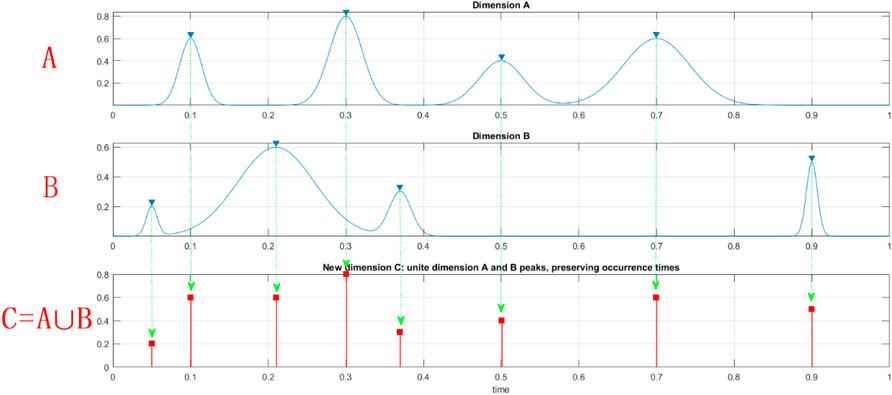
FIGURE 1. Illustration of synthetic $\overrightarrow{\mathit{R}}$ vector construction (process C), using two different dimensional processes’ local maxima and overlapping them in real-time.

Next, a scaling parameter$\mathrm{0}<\lambda \le \mathrm{1}$ is introduced to artificially simultaneously decrease limit values for all response components, namely the new MDOF limit vector $\left({\eta }_X^{\lambda },{\eta }_Y^{\lambda },{\eta }_z^{\lambda },...\right)$ with ${\eta }_X^{\lambda }\equiv \lambda {\bullet \eta }_X$, $\equiv \lambda {\bullet \eta }_Y$, ${\eta }_z^{\lambda }\equiv \lambda {\bullet \eta }_Z$, ... Is introduced. The unified limit vector $\left({\eta }_{\mathrm{1}}^{\lambda },\dots ,{\eta }_N^{\lambda }\right)$ is introduced with each component ${\eta }_j^{\lambda }$ is either ${\eta }_X^{\lambda }$, ${\eta }_Y^{\lambda }$or ${\eta }_z^{\lambda }$ and so on. The latter automatically defines probability $P\left(\lambda \right)$ as a function of $\lambda$, note that $P\equiv P\left(\mathrm{1}\right)$ from Eq. 1. Non-exceedance probability $P\left(\lambda \right)$ can be estimated as follows:

$P\left(\lambda \right)=\mathrm{P}\mathrm{r}\mathrm{o}\mathrm{b}\left\{R_N\le {\eta }_N^{\lambda },\dots ,R_{\mathrm{1}}\le {\eta }_{\mathrm{1}}^{\lambda }\right\}=\mathrm{P}\mathrm{r}\mathrm{o}\mathrm{b}\{R_N\le {\eta }_N^{\lambda }|R_{N-\mathrm{1}}\le {\eta }_{N-\mathrm{1}}^{\lambda },\dots ,R_{\mathrm{1}}\le {\eta }_{\mathrm{1}}^{\lambda }\}\cdot \mathrm{P}\mathrm{r}\mathrm{o}\mathrm{b}\{R_{N-\mathrm{1}}\le {\eta }_{N-\mathrm{1}}^{\lambda },\dots ,R_{\mathrm{1}}\le {\eta }_{\mathrm{1}}^{\lambda }\}={\displaystyle \prod }_{j=\mathrm{2}}^N\mathrm{P}\mathrm{r}\mathrm{o}\mathrm{b}\left\{R_j\le {\eta }_j^{\lambda }|R_{j-\mathrm{1}}\le {\eta }_{\mathrm{1}j-}^{\lambda },\dots ,R_{\mathrm{1}}\le {\eta }_{\mathrm{1}}^{\lambda }\right\}\cdot \mathrm{P}\mathrm{r}\mathrm{o}\mathrm{b}\left(R_{\mathrm{1}}\le {\eta }_{\mathrm{1}}^{\lambda }\right)(3)$

The following outlines the principle behind a cascade of approximations based on conditioning. The first approximation is a one-step memory approximation and thus resembles a Markov chain approximation. However, it is emphasised that this first approximation is not equivalent to such an approximation (Karpa, 2015). In practice, the dependence between the neighbouring $R_j$ is not negligible; thus, the following one-step (will be called conditioning level $k=\mathrm{1}$) memory approximation is introduced:

$\mathrm{P}\mathrm{r}\mathrm{o}\mathrm{b}\left\{R_j\le {\eta }_j^{\lambda }|R_{j-\mathrm{1}}\le {\eta }_{j-\mathrm{1}}^{\lambda },\dots ,R_{\mathrm{1}}\le {\eta }_{\mathrm{1}}^{\lambda }\right\}\approx \mathrm{P}\mathrm{r}\mathrm{o}\mathrm{b}\left\{R_j\le {\eta }_j^{\lambda }|R_{j-\mathrm{1}}\le {\eta }_{j-\mathrm{1}}^{\lambda }\right\}(4)$

for $\mathrm{2}\le j\le N$ (will be called conditioning level $k=\mathrm{2}$). The approximation introduced by Eq. 4 can be further expressed as:

$\mathrm{P}\mathrm{r}\mathrm{o}\mathrm{b}\left\{R_j\le {\eta }_j^{\lambda }|R_{j-\mathrm{1}}\le {\eta }_{j-\mathrm{1}}^{\lambda },\dots ,R_{\mathrm{1}}\le {\eta }_{\mathrm{1}}^{\lambda }\right\}\approx \mathrm{P}\mathrm{r}\mathrm{o}\mathrm{b}\left\{R_j\le {\eta }_j^{\lambda }|R_{j-\mathrm{1}}\le {\eta }_{j-\mathrm{1}}^{\lambda },R_{j-\mathrm{2}}\le {\eta }_{j-\mathrm{2}}^{\lambda }\right\}(5)$

where $\mathrm{3}\le j\le N$ (will be called conditioning level $k=\mathrm{3}$), and so on, see (Karpa, 2015). The motivation is to monitor each independent failure that happened locally first in time, thus avoiding cascading local inter-correlated exceedances.

Eq. 5 presents subsequent refinements of the statistical independence assumption. The latter type of approximations captures the statistical dependence effect between neighbouring maxima with increased accuracy. Since the original MDOF process $\mathit{R}\left(t\right)$ was assumed ergodic and therefore stationary, probability $p_k\left(\lambda \right)≔\mathrm{P}\mathrm{r}\mathrm{o}\mathrm{b}\{R_j>{\eta }_j^{\lambda }|R_{j-\mathrm{1}}\le {\eta }_{j-\mathrm{1}}^{\lambda },R_{j-k+\mathrm{1}}\le {\eta }_{j-k+\mathrm{1}}^{\lambda }\}$ for $j\ge k$ will be independent of $j$ but only dependent on conditioning level $k$. Thus non-exceedance probability can be approximated as in the Naess-Gaidai method, see (Naess and Gaidai, 2009; Gaidai et al., 2018; Gaidai et al., 2020; Gao et al., 2020) where:

$P_k\left(\lambda \right)\approx \exp \left(-{N\bullet p}_k\left(\lambda \right)\right),k\ge \mathrm{1}(6)$

Note that Eq. 6 follows from Eq. 1 by neglecting$\mathrm{P}\mathrm{r}\mathrm{o}\mathrm{b}\left(R_{\mathrm{1}}\le {\eta }_{\mathrm{1}}^{\lambda }\right)\approx \mathrm{1}$, as the design failure probability is usually very small.

Note that Eq. 5 is similar to the well-known mean up-crossing rate equation for the probability of exceedance (Gaidai et al., 2020; Gao et al., 2020; Naess and Gaidai, 2009). There is evident convergence with respect to the conditioning parameter$k$:

$P=\underset{k\to \infty }{\lim }{P}_k\left(\mathrm{1}\right);p\left(\lambda \right)=\underset{k\to \infty }{\lim }{p}_k\left(\lambda \right)(7)$

Note that Eq. 6 for $k=\mathrm{1}$ turns into the well-known non-exceedance probability relationship with the mean up-crossing rate function

$P\left(\lambda \right)\approx \exp \left(-{\nu }^{+}\left(\lambda \right)T\right);{\nu }^{+}\left(\lambda \right)={\int }_{\mathrm{0}}^{\infty }\zeta p_{R\dot{R}}\left(\lambda ,\zeta \right)d\zeta (8)$

where ${\nu }^{+}\left(\lambda \right)$ denotes the mean up-crossing rate of the response level $\lambda$ for the above assembled non-dimensional vector $R\left(t\right)$ assembled from scaled MDOF system response $\left(\frac{X}{{\eta }_X},\frac{Y}{{\eta }_Y},\frac{Z}{{\eta }_Z},\dots \right)$.

Rice’s formula gives the mean up-crossing rate in Eq. 8 with $p_{R\dot{R}}$ being joint probability density for $\left(R,\dot{R}\right)$ with $\dot{R}$ being time derivative$R^{\prime }\left(t\right)$, see (Rice, 1944). Equation 8 relies on the Poisson assumption, which is that up-crossing events of high $\lambda$ levels (in this paper, it is $\lambda \ge \mathrm{1}$) can be assumed to be independent. The latter may not be the case for narrow band responses and higher level dynamical systems that exhibit cascading failures in different dimensions, subsequent in time, caused by intrinsic inter-dependency between extreme events, manifesting itself in the appearance of highly correlated local maxima clusters within the assembled vector $\overrightarrow{R}=\left(R_{\mathrm{1}},R_{\mathrm{2}},\dots ,R_N\right)$.

In the above, the stationarity assumption has been used. The proposed methodology can also treat the non-stationary case. An illustration of how the methodology can be used to treat non-stationary cases is provided as follows. Consider a scattered diagram of $m=\mathrm{1},..,M$ sea states, each short-term sea state having a probability$q_m$, so that${\displaystyle \sum }_{m=\mathrm{1}}^M{q}_m=\mathrm{1}$. The corresponding long-term equation is then:

$p_k\left(\lambda \right)\equiv {\displaystyle \sum }_{m=\mathrm{1}}^M{p}_k\left(\lambda ,m\right)q_m(9)$

with $p_k\left(\lambda ,m\right)$ being the same function as in Eq. 7 but corresponding to a specific short-term sea state with the number $m$.

Model introduction

The Naess-Gaidai extrapolation model (Naess and Moan, 2013; Gaidai et al., 2022; Xing et al., 2022; Xu et al., 2022) is briefly introduced as it will be used as a basis for the failure probability distribution tail extrapolation. The method assumes that the class of parametric functions needed for extrapolation in the general case can be modelled similarly to the relation between the Gumbel distribution and the general extreme value (GEV) distribution. The above introduced $p_k\left(\lambda \right)$ as functions are often regular in the tail, specifically for values of$\lambda$ approaching and exceeding$\mathrm{1}$. More precisely, for $\lambda \ge {\lambda }_{\mathrm{0}}$.The distribution tail behaves similar to $\exp \left\{-{\left(a\lambda +b\right)}^c+d\right\}$ with $a,b,c,d$ being suitably fitted constants for suitable tail cut-on ${\lambda }_{\mathrm{0}}$value. Therefore, one can write;

$p_k\left(\lambda \right)\approx \exp \left\{-{\left(a_k\lambda +b_k\right)}^{c_k}+d_k\right\},\lambda \ge {\lambda }_{\mathrm{0}}(10)$

Next, by plotting $\ln \left\{\ln \left(p_k\left(\lambda \right)\right)-d_k\right\}$ versus $\ln \left(a_k\lambda +b_k\right)$, often a nearly perfectly linear tail behaviour is observed. It is useful to do the optimisation on the logarithmic level by minimising the following error function F with respect to the four parameters$a_k,b_k,c_k,p_k,q_k$:

$F\left(a_k,b_k,c_k,p_k,q_k\right)={{\int }_{{\lambda }_{\mathrm{0}}}^{{\lambda }_{\mathrm{1}}}\omega \left(\lambda \right)\left\{\ln \left(p_k\left(\lambda \right)\right)-d_k+{\left(a_k\lambda +b_k\right)}^{c_k}\right\}}^{\mathrm{2}}d\lambda ,\lambda \ge {\lambda }_{\mathrm{0}}(11)$

with${\lambda }_{\mathrm{1}}$being a suitable distribution tail cut-off value, namely the largest response value, where the confidence interval width is still acceptable. Optimal values of the parameters $a_k,b_k,c_k,p_k,q_k$ may also be determined using a sequential quadratic programming (SQP) method incorporated in the NAG Numerical Library (Numerical Algorithms Group, 2010).

The weight function $\omega$ can be defined as $\omega \left(\lambda \right)={\left\{\ln {\mathrm{C}\mathrm{I}}^{+}\left(\lambda \right)-\ln {\mathrm{C}\mathrm{I}}^{-}\left(\lambda \right)\right\}}^{-\mathrm{2}}$with $\left({\mathrm{C}\mathrm{I}}^{-}\left(\lambda \right),{\mathrm{C}\mathrm{I}}^{+}\left(\lambda \right)\right)$ being a confidence interval (CI), empirically estimated from the simulated or measured dataset, see (Gaidai et al., 2020; Gao et al., 2020; Naess and Gaidai, 2009). When the parameter $c=\underset{k\to \infty }{\lim }{c}_k$ is equal or close to 1, the distribution approaches to the Gumbel distribution.

For any general ergodic process, the sequence of conditional exceedances over a threshold $\lambda$ can be assumed to constitute a Poisson process. However, in general, a non-homogeneous one. Thus, for levels of $\lambda$ approaching $\mathrm{1}$, the approximate limits of a p-% confidence interval (CI) of $p_k\left(\lambda \right)$can be given as follows:

$\mathrm{C}{\mathrm{I}}^{\pm }\left(\lambda \right)=p_k\left(\lambda \right)\left(\mathrm{1}\pm \frac{f\left(p\right)}{\sqrt{\left(N-k+\mathrm{1}\right)p_k\left(\lambda \right)}}\right).(12)$

with $f\left(p\right)$ being estimated from the inverse normal distribution, for example, $f\left(\mathrm{90}\%\right)=1.65$, $f\left(\mathrm{95}\%\right)=1.96$. With $N$ being the total number of local maxima assembled in the analysed vector $\overrightarrow{R}$.

Note that the authors have successfully verified the accuracy of the Naess-Gaidai extrapolation model in previous years for a large variety of one-dimensional dynamic systems (Gaidai et al., 2020; Gao et al., 2020; Naess and Gaidai, 2009; Sun et al., 2022).

Data introduction

This section intends to illustrate the efficiency of the above-described methodology, utilising the method to predict the extreme wind speeds at a group of selected measured sites in Southern Norway near the Landvik wind station. The five wind measurement locations are Landvik, Kjevik, Lindesnes Fyr, Lista Fyr and Oksøy Fyr. Their measured daily highest daily wind cast speeds are defined as five environmental system components (dimensions) $X,Y,Z,\dots$, thus constituting an example of a five-dimensional (5D) environmental system. The definition of design values is problem-specific and has to be appropriately considered by the end-user. As an example for this paper, the unidimensional design value for each dimension, i.e., the value in which the wind speed is unacceptable at each location, is chosen as twice the maximum daily highest daily wind cast speed during the observation period 2010-2020 for each of the five selected wind measurement locations.

Figure 2 presents wind measurement locations according to the Norwegian Meteorological Institute, 2021. The blue circle indicates the area of interest. The daily largest wind cast speed at the Landvik location during the years 2010–2020 is shown in Figure 3.

$X\to \frac{X}{{\eta }_X},Y\to \frac{Y}{{\eta }_Y},Z\to \frac{Z}{{\eta }_Z},\dots (13)$

making all five responses non-dimensional and having the same failure limit equal to 1.

FIGURE 2

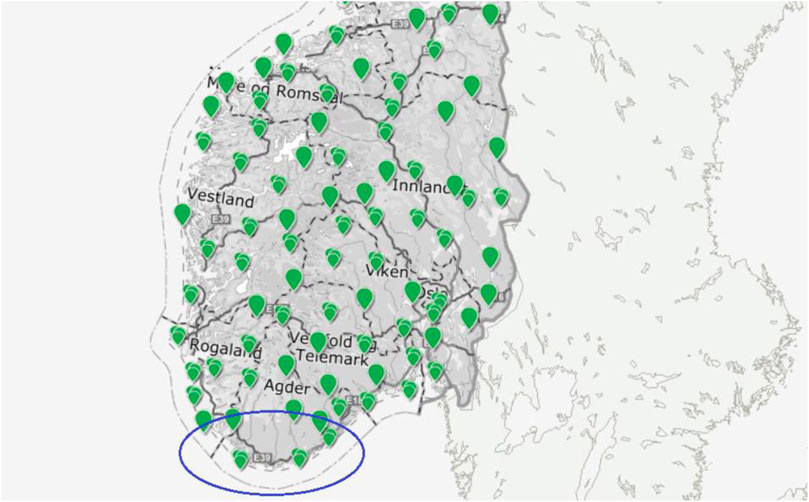
FIGURE 2. Wind speed measurements locations according to Norwegian Meteorological Institute. The blue circle indicates the area of interest.

FIGURE 3

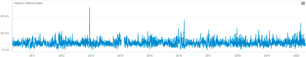
FIGURE 3. Daily largest wind cast speed at Landvik location during the years 2010–2020 (Norwegian Meteorological Institute, https://seklima.met.no/). In order to unify all five measured time series $X,Y,Z$,. The following scaling was performed.

Next, all the local maxima from five measured time series are merged into one single time series by keeping them in time non-decreasing order: $\overrightarrow{R}=\left(\left\{X_{\mathrm{1}},Y_{\mathrm{1}},Z_{\mathrm{1}},\dots \right\},\dots ,\left\{X_N,Y_N,Z_N,\dots \right\}\right)$ with each set $\left\{X_j,Y_j,Z_j,\dots \right\}$ being sorted according to non-decreasing times of occurrence of these local maxima.

Figure 4 presents an example of the non-dimensional assembled vector $\overrightarrow{R}$, consisting of assembled local maxima of raw daily largest wind cast speed data. The failure probability distribution tail extrapolation was performed towards 100 years return period. Note that vector $\overrightarrow{R}$ does not have physical meaning on its own, as it is assembled of completely different response components. The index $j$ is just a running index of local maxima encountered in a non-decreasing time sequence.

FIGURE 4

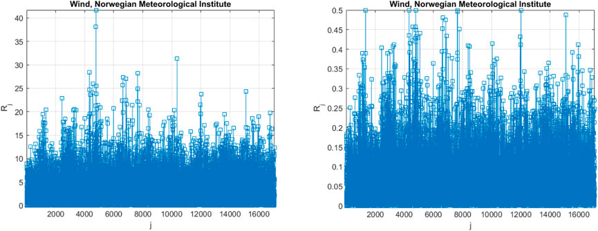
FIGURE 4. Left: unscaled raw daily largest wind cast speed data [m/sec], Right: scaled non-dimensional assembled 5D vector $\overrightarrow{\mathit{R}}$.

Figure 5 presents extrapolation according to Eq. 9 towards failure state with 25 years return period, which is 1, and somewhat beyond, $\lambda =\mathrm{0.15}$ cut-on value was used. The dotted lines indicate extrapolated 95% confidence interval according to Eq. 10. According to Eq. 6, $p\left(\lambda \right)$ is directly related to the target failure probability $\mathrm{1}-P$ from Eq. 1. Therefore, in agreement with Eq. 6, the system failure probability, $\mathrm{1}-P\approx {\mathrm{1}-P}_k\left(\mathrm{1}\right)$ can be estimated. Note that in Eq. 5, $N$ corresponds to the total number of local maxima in the unified response vector$\overrightarrow{R}$. The conditioning parameter$k=\mathrm{4}$ was found to be sufficient due to occurrence of convergence with respect to $k$; see Eq. 6. Figure 5 exhibits a relatively narrow 95% CI; the latter is due to a substantial amount of data used in this study, namely the recent 10 years of continuously measured data.

FIGURE 5

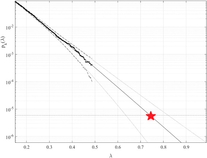
FIGURE 5. Extrapolation of ${\mathit{p}}_{\mathit{k}}\left(\mathit{\lambda }\right)$ towards critical level corresponding to 100 years return period (indicated by a star) and beyond,$\mathit{k}=\mathit{6}$. The extrapolated 95% CI is indicated by dotted lines.

As demonstrated, while being novel, the above-described methodology has a clear advantage in efficiently utilising the available measured data set. This is due to its ability to treat system multi-dimensionality, as well as being able to perform accurate extrapolation based on a relatively limited data set.

Conclusion

Classic reliability methods dealing with time series do not have the advantage of dealing efficiently with systems possessing high dimensionality and cross-correlation between different system responses. The key advantage of the introduced methodology is its ability to study the reliability of high-dimensional non-linear dynamic systems.

This paper studied the Norwegian highest largest wind cast speeds data set, in the region near Landvik wind station, observed during the recent decade 2010-2020. A novel environmental reliability method was applied to predict the occurrence of extreme winds in the area of interest within the time horizon of the next 100 years. It is shown that the proposed method produced a reasonable confidence interval. Thus, the suggested methodology may become an appropriate tool for various non-linear dynamic systems reliability studies. Both measured and numerically simulated time series responses can be analysed. Further, unlike other reliability methods, the new method does not require restarting numerical simulation each time it fails, for example, in the case of Monte Carlo simulations. Finally, the suggested methodology can be used in a wide range of engineering areas of applications. [Andersen and Jensen, 2014, Ellermann, 2008, Falzarano et al., 2012, Su, 2012.

Data availability statement

The original contributions presented in the study are included in the article/Supplementary Material, further inquiries can be directed to the corresponding author.

Author contributions

All authors listed have made a substantial, direct, and intellectual contribution to the work and approved it for publication.

Funding

This study was partially supported by the National Natural Science Foundation of China [grant numbers: 52071203]; the authors would like to express their gratitude for supporting the Fishery Engineering and Equipment Innovation Team of Shanghai High-level Local University.

Conflict of interest

The authors declare that the research was conducted in the absence of any commercial or financial relationships that could be construed as a potential conflict of interest.

Publisher’s note

All claims expressed in this article are solely those of the authors and do not necessarily represent those of their affiliated organizations, or those of the publisher, the editors and the reviewers. Any product that may be evaluated in this article, or claim that may be made by its manufacturer, is not guaranteed or endorsed by the publisher.

References

Andersen, J., and Jensen, J. J. (2014). Measurements in a container ship of wave-induced hull girder stresses in excess of design values. Mar. Struct. 37, 54–85. doi:10.1016/j.marstruc.2014.02.006

CrossRef Full Text | Google Scholar

Choi, S-K., Grandhi, R. V., and Canfield, R. A. (2007). Reliability-based structural design. London: Springer-Verlag.

Google Scholar

Ditlevsen, O., and Madsen, H. O. (1996). Structural reliability methods. Chichester (UK): John Wiley & Sons.

Google Scholar

Ellermann, K. (2008). IUTAM symposium on fluid-structure interaction in ocean engineering. China: Springer, 45–56. Non-linear dynamics of offshore systems in random seas.

Google Scholar

Eryilmaz, S., and Kan, C. (2020). Reliability based modeling and analysis for a wind power system integrated by two wind farms considering wind speed dependence. Reliability Engineering & System Safety 203, 1.

CrossRef Full Text | Google Scholar

Falzarano, J., Su, Z., and Jamnongpipatkul, A. (2012). “Application of stochastic dynamical system to non-linear ship rolling problems,” in Proceedings of the 11th international conference on the stability of ships and ocean vehicles (Athens, Greece: National Technical University of Athens).

Google Scholar

Gaidai, O., Wang, F., Wu, Y., Xing, Y., Medina, A., and Wang, J. (2022). Offshore renewable energy site correlated wind-wave statistics. Probabilistic Eng. Mech. 68, 103207. doi:10.1016/j.probengmech.2022.103207

CrossRef Full Text | Google Scholar

Gaidai, O., Xu, X., Naess, A., Cheng, Y., Ye, R., and Wang, J. (2020). Bivariate statistics of wind farm support vessel motions while docking. Ships offshore Struct. 16 (2), 135–143. doi:10.1080/17445302.2019.1710936

CrossRef Full Text | Google Scholar

Hansen, A. (2020). The three extreme value distributions: An introductory review. Front. Phys 8, 604053. doi:10.3389/fphy.2020.604053

CrossRef Full Text | Google Scholar

Kan, C., Devrim, Y., and Eryilmaz, S. (2020). On the theoretical distribution of the wind farm power when there is a correlation between wind speed and wind turbine availability. Reliability Engineering & System Safety 203, 1.

CrossRef Full Text | Google Scholar

Karpa, O. (2015). Development of bivariate extreme value distributions for applications in marine technology. Trondheim: Norwegian University of Science and Technology. PhD thesis.

Google Scholar

Madsen, H. O., Krenk, S., and Lind, N. C. (1986). Methods of structural safety. Englewood Cliffs: Prentice-Hall.

Google Scholar

Majumdar, S. N., Pal, A., and Schehr, G. (2020). Extreme value statistics of correlated random variables: A pedagogical review. Phys. Rep. 840, 1–32. doi:10.1016/j.physrep.2019.10.005

CrossRef Full Text | Google Scholar

Melchers, R. E. (1999). Structural reliability analysis and prediction. New York: John Wiley & Sons.

Google Scholar

Naess, A., and Gaidai, O. (2009). Estimation of extreme values from sampled time series. Struct. Saf. 31 (4), 325–334. doi:10.1016/j.strusafe.2008.06.021

CrossRef Full Text | Google Scholar

Naess, A., Leira, B. J., and Batsevych, O. (2009). System reliability analysis by enhanced Monte Carlo simulation. Struct. Saf. 31, 349–355. doi:10.1016/j.strusafe.2009.02.004

CrossRef Full Text | Google Scholar

Naess, A., and Moan, T. (2013). Stochastic dynamics of marine structures. Cambridge: Cambridge University Press.

Google Scholar

Norwegian Meteorological Institute (2021). Norwegian meteorological Institute. Available at: https://seklima.met.no/.

Google Scholar

Numerical Algorithms Group (2010). NAG toolbox for matlab. Oxford, UK: NAG Ltd.

Google Scholar

Rice, S. O. (1944). Mathematical analysis of random noise. Bell Syst. Tech. J. 23, 282–332. doi:10.1002/j.1538-7305.1944.tb00874.x

CrossRef Full Text | Google Scholar

Su, Z. (2012). Non-linear response and stability analysis of vessel rolling motion in random waves using stochastic dynamical systems. Texas: Texas University.

Google Scholar

Sun, J., Gaidai, O., Wang, F., Naess, A., Wu, Y., Xing, Y., and Chen, M. (2022). Extreme riser experimental loads caused by sea currents in the Gulf of Eilat. Probabilistic Eng. Mech. 68, 103243. doi:10.1016/j.probengmech.2022.103243

CrossRef Full Text | Google Scholar

Thoft-Christensen, P., and Murotsu, Y. (1986). Application of environmental systems reliability theory. Berlin: Springer-Verlag.

Google Scholar

Xing, Y., Gaidai, O., Ma, Y., Naess, A., and Wang, F. (2022). A novel design approach for estimation of extreme responses of a subsea shuttle tanker hovering in ocean current considering aft thruster failure. Appl. Ocean Res. 123. doi:10.1016/j.apor.2022.103179

CrossRef Full Text | Google Scholar

Xu, X., Wang, F., Gaidai, O., Naess, A., Xing, Y., and Wang, J. (2022). Bivariate statistics of floating offshore wind turbine dynamic response under operational conditions. Ocean. Eng. 257, 111657. doi:10.1016/j.oceaneng.2022.111657

CrossRef Full Text | Google Scholar

Zheng, C., Liang, F., Yao, J., Dai, J., Gao, z., Hou, T., and Xioan, F. (2020). Seasonal extreme wind speed and gust wind speed: A case study of the China seas. J. Coast. Res. 99, 435–438. doi:10.2112/SI99-059.1

CrossRef Full Text | Google Scholar

Zheng, C., Xiao, Z., Peng, Y., Li, C., and Du, Z. (2018). Rezoning global offshore wind energy resources. Renew. Energy 129, 1–11. doi:10.1016/j.renene.2018.05.090

CrossRef Full Text | Google Scholar