Field trials testing material composition and surface complexity and the effects on benthic faunal recruitment at a cold-water coral reef site

Reef habitats of the cold-water coral Desmophyllum pertusum in the Skagerrak have been damaged until near extinction by bottom trawling and other anthropogenic impacts over the last decades. There is, however, one site with a thriving reef that brings hope for potential recovery. A large-scale restoration project has been launched, and to find the optimal material composition for the artificial reefs to be deployed we tested three concrete mixes against standard Portland cement as controls, and two different surface textures with different levels of complexity in a field settling experiment. The mixed concrete panels had different ratios of ground granulated blast furnace slag and silica oxide added, components that have been shown to increase compressive strength and longevity of concrete in the marine environment. Panels were deployed close to a live reef site and left submerged for 19 months. Recruitment of reef associated fauna was generally high on all panels. Surface complexity had a significant effect on diversity and species richness, with higher values on the more complex substrates. The position of the panels (side and level above seafloor) was associated with a significant effect on coverage, diversity, and richness. The concrete mix had less effect on coverage and diversity of associated fauna, however, panels with the highest level of added silica oxide had significantly lower values. No recruitment of D. pertusum larvae were observed. The results show that surface complexity is more important than material composition for the recruitment of benthic invertebrates, and one can therefore put more focus on complexity and material durability when constructing artificial reefs.

Introduction

The scleractinian coral Desmophyllum pertusum (Linnaeus, 1758)—previously known as Lophelia pertusa—is the deep-sea coral creating the largest reef habitats, stretching over several square kilometers if left undisturbed. It thus offers a complex habitat for associated fauna at landscape scales (Buhl-Mortensen et al., 2010). Cold-water coral (CWC) reef habitats are biodiversity hotspots with a biodiversity on par with tropical coral reefs, although usually made up by single or a few species of scleractinian corals, in contrast to tropical reefs that consist of a multitude of coral species in addition to the diversity of associated fauna. The associated biodiversity in CWC habitats is high, with most of the fauna associated with the dead basal parts of the reefs, while only a few species are found in the living parts of the reefs (Jensen and Frederiksen, 1992; Bourque and Demopoulos, 2018). More than 1800 species have been recorded associated with D. pertusum habitats in the NE Atlantic, and 2700 species globally (Roberts and Cairns, 2014). The high biodiversity stems from the effect the complex reef matrix have on the passing currents. Their three-dimensional skeletal matrix induces precipitation of particulate organic material (POM) as well as pelagic larvae from the passing water masses, enhancing both nutrient availability and fauna within the reef (Maier et al., 2023). This baffling of particulate matter is also what is behind the build-up of coral mounds (Roberts et al., 2006; Douarin et al., 2014). This way of modulating the environment and nutrient cycling is defined as autogenic engineering (Jones et al., 1994), and D. pertusum can thus be defined as an ecosystem engineer.

The highly complex landscape created by this coral is used by commercially important species of fish that seek refuge and food within the reef habitat (Husebø et al., 2002; Henderson et al., 2020). Fishermen have reported that catches have declined in areas where the reef habitat has been damaged (Fosså et al., 2002). Trawling impacts to CWC reef habitats have been compared to forest clear-cutting and recovery after damage is slow to non-existing (Watling and Norse, 1998; Huvenne et al., 2016). Deep-sea corals are slow-growing and recovery to pre-damage complexity may take centuries. The slow growth rate is also countered by a continuous rate of bioerosion, such that net reef growth is slower than the extension rates of individual polyps (Büscher et al., 2019; Järnegren and Kutti, 2014). While coral calice extension in D. pertusum can be c. 10 mm year^-1 the reef growth can be half that number, 5 mm year^-1. However, when the three-dimensional complexity is completely lost, recovery is unlikely to occur at all.

In the 2022 OSPAR Status Assessment (OSPAR, 2022) for Lophelia pertusa the overall status was found to be poor in all OSPAR regions. It is estimated that L. pertusa reef coverage in Norway has declined by 30%–50% due to fishery impacts (Fosså et al., 2002). In a study in the Skagerrak conducted in 2004 and 2009, the biodiversity in a number of sampling sites overlapping with the historical sampling conducted by Jägerskiöld in 1921–1938 revealed that only 32.8% of species were observed in both the recent and historical samples, with 60.8% only present in the historical samples (Jägerskiöld, 1971; Obst et al., 2018). A majority of the observed species showed a decline over time, with especially rare species lost. There is an apparent decline in biodiversity in the Skagerrak in general. Restoring CWC habitats could help turn this decline and assist in restoring biodiversity.

In response to the global loss of biodiversity, the Conference of the Parties (COP) to the Convention on Biological Diversity (CBD) established twenty ambitious targets to protect biodiversity in the Aichi Biodiversity Targets (Resolution 65/161, CBD website). Target 11 aimed to protect 10 per cent of coastal and marine areas by 2020, with special focus on areas of particular importance for biodiversity and areas that provide important ecosystem services. The 10 per cent was surpassed for marine areas under national jurisdiction in 2017, reaching 15.9 per cent, while areas beyond national jurisdiction are lagging with only 1.8 per cent protected (Gannon et al., 2017). In Sweden, the establishment of the Natura 2000 Kosterfjord-Väderöfjord area in 2001, and the inauguration of the Kosterhavet National Park in 2009—including both terrestrial and marine areas—has put protection in place for this unique and diverse water body along the coastline.

In addition to the establishment of Marine Protected Areas (MPAs) the recognition that CWC reef habitats have been so severely degraded over the last decades that active restoration measures are needed has prompted several restoration attempts in Europe. This is in line with the call by the UN Resolution 73/284 (United Nations General Assembly, 2019), to “prevent, halt and reverse the degradation of ecosystems worldwide”. The years 2021–2030 have been declared the United Nations Decade on Ecosystem Restoration. The EU LIFE fund Nature and Biodiversity has funded several large-scale attempts at restoring deep-sea corals, including the current project LIFE Lophelia.

Within the present area in Skagerrak, recovery has only occurred where three-dimensional substrates in the form of dead coral framework remained. No recovery has been seen in areas where only coral rubble is left. Presence of live corals that maintain habitat 3D complexity is important for the maintenance of the reef associated fauna. Without live corals the habitat will eventually lose that complexity and the associated fauna will diminish. Most coral larvae require elevated substrates free from sediment cover for successful recruitment (e.g., Gilmour, 1999; Moeller et al., 2017). Sedimentation rates are comparably high in this coastal area, but the high current speeds keep some of the protruding surfaces clean. The largest of the reefs in the Natura 2000 Kosterfjord-Väderöfjord area, the Väderö reef, is today estimated to be approximately 300 m², while the surrounding area with coral rubble extends to over 20,000 m² (Norlinder et al., 2025), indicating that the live reef historically has been substantially larger. The reef area has been protected from fishery impacts since 2001 and has since then gone from no observed live coral cover in 1998 (Lundälv and Jonsson, 2000), to dense mats of young colonies observed in 2013 (Jonsson, 2014). Today the colonies are thriving, with dense healthy polyps. This prompted us to use active measures to restore some of the lost complexity to allow for further expansion of live coral cover in the area.

To provide a solid base for larval recruitment that has the potential to offer long-term support for growing corals, we needed to find a material composition that will last for up to a century in the marine environment. Concrete is the most tested material for marine applications, and the concrete structures with the highest known longevity in marine settings are the piers built by the Romans (Oleson et al., 2004; Jackson et al., 2018). These structures have lasted for two millennia, eroded, although still rock hard at their core. The Romans used volcanic materials mixed with lime that produced a calcium-aluminum-silicate-hydrate (C-A-S-H) binder with a slow strength build-up, but which continued to harden while submerged in seawater ending up harder than concrete made from standard Portland cement (PC), and having self-repairing properties (Oleson et al., 2004). Modern materials with similar properties as the volcanic pozzolan materials are metallurgic slag and Ground Granulated Blast Furnace Slag (GGBFS), both biproducts from the metal industries (Table 1). GGBFS is known to improve strength and durability of concrete, as well as reducing the carbon footprint of the final product (Song and Saraswathy, 2006). It also protects reinforcement bars within the concrete due to the higher fine particulate silica content that gives the concrete a denser microstructure and reduces chloride intrusion (Bhat and Tengli, 2019). A close to 50:50 mix of standard Portland cement and GGBFS is shown to produce the highest compressive strength (Osmanovic et al., 2018), while protection from chloride intrusion has a positive linear relationship with GGBFS and silica content (Bhat and Tengli, 2019). In the Netherlands GGBFS has been used in marine concrete structures since the 1920s, and since 1986 the Dutch concrete technology standard recommend using CEM III/B for the marine environment, with a GGBFS content of 70–72 per cent (Polder et al., 2014; Gulikers, 2016). The Netherlands is depending heavily on concrete barriers, and this long-term use of CEM III/B in marine applications vouches for the longevity aspect. There have also been trials with GGBFS inclusion in concrete for the purpose of enhancing recruitment of benthic fauna on artificial reefs that has shown promising results, with some of the effect attributed to the lower pH of concrete due to higher silica and aluminum content (Perkol-Finkel and Sella, 2014; Sella and Perkol-Finkel, 2015; Ly et al., 2021). Thus, there is a potential for a triple-win situation using GGBFS in artificial reefs: 1) enhanced material longevity, 2) enhancement of the recruitment of benthic fauna, and 3) reduced carbon footprint.

Table 1

Table 1. Comparison of the mineral composition of different cementitious materials and slag: PC = regular Portland Cement; GGBFS 1 = Ground Granulated Blast Furnace Slag sourced from Thomas Cement; GGBFS 2 = sourced from SSAB Merox; MS = Metallurgic Slag sourced from Höganäs AB; POZZ = volcanic pozzolan material as described in Oleson et al. (2004).

Within the project LIFE Lophelia we aim at restoring the habitat complexity lost at six sites within the Natura 2000 Kosterfjord-Väderöfjord area in Skagerrak through deployment of artificial reefs (ARs). To find the optimal mix of concrete for recruitment of D. pertusum and associated benthic fauna we tested three mixes of concrete against standard Portland cement as controls. The testing was done in a two-part trial where the mixes was tested both in coral larval settling trials in the laboratory, and in field trials where the effect of mix on potentially both coral larvae and associated fauna could be tested. In this paper we present the results of the field trial while the results from the laboratory are presented in a companion paper in this same issue (Strömberg et al., 2025). The three mixes contained different ratios of GGBFS and silica oxide (SiO₂). For each concrete mix we also tested two levels of surface complexity. Settling panels with the mixes were deployed at the Väderö reef site in the most southern part of the Natura 2000 area and were retrieved after 19 months. The panels were examined regarding both mobile and sessile fauna and assessed for differences in faunal coverage and diversity.

Materials and methods

Study area

Along the west coast of Sweden there is a deep trough, channeling deep oceanic water from the North Atlantic via the Norwegian Trench and into the coastal area between the Koster Islands and mainland Sweden (Figures 1A,B). This inflow of deep Atlantic waters brings deep-sea organisms into the area, including the reef-building scleractinian coral Desmophyllum pertusum. Within this area there are six sites with known occurrences of D. pertusum (Figure 1A). Today the sites consist of mostly coral rubble or small lumps of dead coral skeleton, however, at one site there is a thriving reef. The Väderö reef is situated at a constriction and sill at the very southern end of the Koster Trough. Current speeds are high, making it a suitable habitat for corals. There is a large coral mound roughly 90 m across and 10–15 m high, indicating a long growth period for the reef. The reefs in the area were established sometime after the last glaciation (Frank et al., 2011; Henry et al., 2014), however, the exact age of the reef is not known. In 2021 the area with live coral colonies was estimated to be 324 m², and the surrounding area with coral rubble to be 20,361 m² (Norlinder et al., 2025), covering the coral mound and extending approximately 100 m south and north of the mound (Figure 1C). The live coral colonies are gathered at the western slope of the mound. The original extent of the live reef is difficult to estimate, since coral rubble has probably been dragged along the bottom with trawling gear while trawling was still allowed in the area. The site has been protected from trawling since 2001 when the Natura 2000 Kosterfjorden-Väderöfjorden area was established. Strictly regulated trawling is allowed in the Natura 2000 area in general, with delimited areas within the general area closed for trawling, and since October 2021 all types of fisheries are banned.

Figure 1

Figure 1. (A) Map of the area with the six restoration sites marked in red. The present study was carried out at the southernmost site, Väderö Islands (6). The orange line demarks the Natura 2000 Kosterfjorden-Väderöfjorden; green line demarks the Kosterhavet Marine National Park; dashed green line the Väderö Nature reserve. TML = Tjärnö Marine Laboratory, a research station belonging to the University of Gothenburg. (B) The area is situated in Skagerrak, on the Swedish west coast close to the Norwegian border. (C) The bathymetry of the Väderö reef site. The white line surrounds the area with coral rubble around the coral mounds, and the asterisk marks the area with live coral colonies. The rack was deployed 20-40 m south of the live corals. Depth contours at 5 m intervals.

No live corals were observed when the reef was first surveyed with ROV (Remotely Operated Vehicle) in 1998 (Lundälv and Jonsson, 2000), although the survey was limited in extent and live corals could have been missed. Previous observations of live corals were 20–30 years prior during scientific sampling (e.g., Jägerskiöld, 1971). At a revisit in the area in 2013 (Jonsson, 2014) dense mats of young colonies were observed, and at later revisits these corals have grown into dense colonies and apparently thrive in the area. In 2013 the area with live corals was estimated to between 10 × 10 m and 20 × 20 m.

Preparation of settling panels

In dialogue with Thomas Concrete Group AB’s cement laboratory (C-Lab, Gothenburg, Sweden), we chose four mixes of concrete to test. One standard Portland cement mix (CEM I 42.5 N SR3 MH/LA) as a control, and three mixes with different ratios of Ground Granulated Blast Furnace Slag (GGBFS) and silica oxide (SiO₂, Table 2). CEM I contain an additive of calcium sulphate (CaSO₄, gypsum) that function as a retarder and controls shrinkage during curing. The origin of the GGBFS (SS-EN 15167-1) accessed via Thomas Cement Group is the metal industries in Bremen, Germany, and it is a latent cementitious material that needs to be combined with calcium oxide (CaO, lime) to activate the curing reactions. The silica oxide was added to the concrete to reduce chloride infiltration and protect the reinforcement bars in the artificial reefs (ARs), as well as to lower the pH of the final product. Silica oxide is an acidic oxide and mix 3 (M3) had high enough silica oxide content to reduce the pH of the cured concrete by one pH unit to test whether recruitment would be enhanced with lower pH. A standard silicious sand was added to the mixes.

Table 2

Table 2. Three mixes were compared to a standard Portland Cement (PC, CEM I 42.5 N SR3 MH/LA). Explanations: GGBFS = Ground Granulated Blast Furnace Slag; SiO = Silica Oxide (SiO₂); Glenium = MasterGlenium 5118 superplasticizer.

C-Lab made concrete prisms with the four mixes and performed tests of compressive strength at days 2, 7, and 28 (Supplementary Figure S2; Supplementary Table S2). In addition, they did pH tests at 28 days by grinding the cured concrete, mixing with deionized water (9 g water per 100 g concrete), and measuring the mix with a pH probe (Table 2).

The dry goods were mixed at the C-Lab and delivered to us in buckets for further processing, adding up to 10 L per mix of dry content. We added the recommended amount of water and Master Glenium 5118, a superplasticizer (based on a polycarboxylate ether) used to reduce water content and improve workability. This additive is necessary when cement mixtures for casting ARs are delivered in a cement truck, and we wanted to add it to the test mixtures to get the same mix as the final product. The Master Glenium was added to the water before mixing it with the dry goods.

A base of wet cement was added in a frame, producing panels that were c. 5 × 10 cm, and to a height of c. 2 cm. On top of that base was added either a mix of wet cement and small pieces of metallurgic slag (5–10 mm, Petrit-E delivered by Höganäs Sweden AB), or a piece of wrinkled jute cloth drenched in wet cement, to create two different types of complex surfaces. Using the same four cement mixes to mix with the slag or jute assured that testing was done on the mixes, not the slag or jute per se. Small amounts of water were added to the mixes as the slag or jute was added to get it completely covered, however, care was taken to maintain a ‘dry’ mix that kept its shape. The total height of the panels was 3–4 cm as the surface textures were added. Casting was done during January and February 2022. The slag and jute were divided equally over the four mixes with 28 replicate panels per mix and surface combined (Table 3-A).

Table 3

Table 3. Number of replicates per mix and per surface (slag or jute) before deployment (A), and number of replicates after retrieval (B).

The panels were subsequently mounted on a rack made from 4 aluminum frames conjoined to produce a square rack (Figure 2). Each frame was 203 × 95 cm long, made of square 3 × 3 cm metal bars. The end bars were used to attach them to each other, and each frame had an additional 7 bars for mounting the panels, fitting 56 panels per side. The distance between bars were 22 cm. We mounted the panels pairwise on both sides of the bars at four different levels above seafloor using cable ties. The panels were mounted at c. 15, 30, 60, and 75 cm above seafloor, with row 1 at the top and row 4 at the bottom. The top and bottom levels (rows) were mostly on the mark; however, the two middle rows were not possible to get at the same level due to different placing of the holes for attachment, or because some of the holes had been closed by calcified fauna during previous deployments of the frames. The levels of row 2 and 3 was thus overlapping. The panels were haphazardly placed within sides and levels, to get an as even allotment of each mix and surface on each side and row as possible.

Figure 2

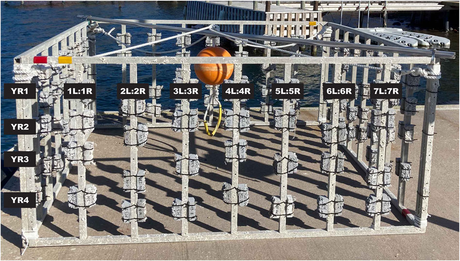
Figure 2. Rack before deployment. The sides were marked with colored reflective tape: yellow+red (YR); green (G); yellow (Y); red (R). To keep track of the individual panels the levels (rows) were coded YR1; YR2; YR3; YR4. The bars were coded 1 through 7, and each individual panel was coded as 1L (left side) or 1R (right side), also adding the mix and surface (slag vs. jute). The coding for the upper left panel was thus YR1-1L-M2-SLAG, [side+level]-[bar 1+left]-[mix]-[surface]. This coding has been used throughout the analyses with mix, surface, side, and row being the main factors. The panels were mounted at c. 15, 30, 60, and 75 cm above seafloor.

Deployment

The rack was deployed April 11^th, 2022, at the most southern site aimed for restoration, Väderö Islands. The rack was transported to the site onboard R/V Nereus and deployed just south of the main coral mound at 58°35.240′N, and 011°04.870′E at a depth of 94 m. The seafloor at the deployment site was inspected by means of a Remotely Operated Vehicle (ROV, Ocean Modules V8 M500) and was found to be current swept, with coral rubble and low-relief dead coral framework covered in hydroids and other fauna. Nearby there were higher-relief dead coral framework. There were no live corals noted in the immediate vicinity, however, the rack was placed c. 20–40 m south of the area with live corals. After successful deployment the orientation of the rack was checked by facing the ROV towards the side marked with red reflective tape, and the heading was noted to be c. 200°SW (Figure 3). The rack was left on the seafloor for 19 months.

Figure 3

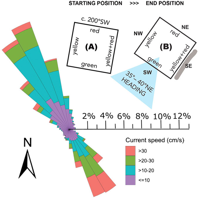
Figure 3. Main current directions at the deployment site Väderö Islands. (A) The rack’s orientation at deployment. When the ROV was facing the red side, the heading was c. 200°SW; (B) Orientation at retrieval. The heading of the ROV facing the green side was 35°–40°NE (marked with a blue arrowhead). The rack had rotated and moved slightly over time. There was a small mound of sediments (grey line) and coral rubble in front of the southeast-facing side (yellow+red, YR) as the rack had been pushed by the currents, indicating the direction of the movement (southeast), correlating with the direction of the strongest currents. The current rose is based on actual measured current direction and speed (cm/s) at the site from four 2–3 months long ADCP deployments during 2020–2023. North facing upwards.

Retrieval

On November 8^th, 2023, the rack was retrieved from the site using R/V Nereus and the same ROV. The orientation was checked again before attaching the wire to the rack, and the heading facing the green side was noted to be 35°–40°NE (Figure 3). A small mound of sediments and coral rubble was seen in front of the yellow+red (YR) side of the rack, suggesting the rack had been rotated and moved a small distance from its original position. The main current directions in the area are northwest and southeast, following the direction of the trough. The stronger currents (30 cm s^-1) were associated with the southeast direction, while the more frequent northwest direction more commonly was in the 10–20 cm s^-1 range (Nestorowicz et al., 2025).

As the rack was hauled onboard it was photo documented before removing the panels (image in Supplementary Material, p. 1). All panels were removed from the rack in systematic order from left to right, with two rows of panels gathered per tray with an inserted grid of compartments made of fine plastic mesh (mosquito net). The trays had been filled with deep water in the morning before departure, coming from the water intake at 45 m depth in the fjord outside the Tjärnö Marine Laboratory. Lost panels were noted, and an empty space left in the inserts in the trays. In all, there were 24 panels lost, leaving 200 panels to be analyzed (Table 3-B). The trays with panels were taken back to the laboratory, a 2:30 h journey. The trays were put on flow-through with deep water upon arrival. Documentation and identification of live material was chosen rather than fixing the samples in ethanol at retrieval. One can learn more about species interactions and how organisms use the substrates by observing them live on the panels, especially the mobile fauna. This can be valuable information when designing ARs.

It should be noted that the jute cloth that was added to the panels had been lost at some point, and only a few tufts of fiber remained on the panels. As the panels were deployed and the jute was soaking up water and swelled, it probably came lose. The timeframe for this is unknown. The strong currents swept the cloths away, leaving a less complex surface than intended.

Documentation and identifications

In the following days, starting November 14th, the panels were photo documented with a Canon EOS 5D Mark II and the fauna identified. The camera was mounted on a stand with a graded leverage bar so that the level of the camera above the panel could be fixed at the same level for every photo shoot. When the zoom lens was used (Canon ZOOM lens 24–70 mm, 1:2.8) for overview photos the lens was set at 70 mm to standardize the photos, and the grid in the LCD window of the camera was used to position the panels centrally in each photo. When the macro lens was used (Canon Macro EF 100 mm, f1:2.8) it was set to cover 1/3 of the panel, and photos were systematically taken in the same order. A piece of a ruler was used for scale in the first photo of each panel. Starting with overview photos with the zoom lens, followed by macro photos for close-ups. Photos were always taken at several focal planes to be able to get all fauna in focus. The first 41 panels were analyzed more thoroughly under the stereo magnifier to get acquainted with the species present. Some of the fauna was photographed under an Olympus BX51 stereo magnifier equipped with a Canon EOS 5D Mark III to get better images for identifications and get a reference gallery of species. The remaining panels were only photo documented, and identifications were done from the photos. The photo documentation of panels was finished 1 month later, on December 14th. One person did all identifications so there was no inter reader variability added. When the photo documentation was finished the analysis was performed in ImageJ/Fiji (version 2.14.0/1.54f, Schindelin et al., 2012), using the Grid and Cell Counter plug-ins to be able to calculate per cent coverage (see example of panel with grid overlay on Supplementary Figure S1). A printout of each panel with the grid overlay was used to keep track and make notes of the species observed. Identifications were supported by all the images taken per panel, both overviews and close-ups, although the quantifications were based on the fauna visible in the chosen image with the grid (see Supplementary Figure S1, and example images in Supplementary Material p. 2).

The identified species were checked against the World Register of Marine Species’ database (WoRMs Editorial Board, 2024) to get the proper nomenclature, and against the Swedish Species Information Centre hosted by the Swedish University of Agricultural Science (SLU Artdatabanken, 2024) to check whether the species had been reported in the area previously.

Quantifications

Colonial organisms were counted by number of cells in the grid where they were present, disregarding the coverage within each cell. Most of the cells had, however, a dense cover of colonies, and since several species were present in many cells the total coverage could exceed 100% for each panel. Barnacles, serpulids, and anomiids were also quantified by coverage even though they are solitary, since they can grow large, extending beyond a single cell of the grid and provide potential substrate for secondary recruitment. Individuals of solitary sessile and mobile organisms were counted, and later recalculated to per cent coverage by dividing the total number of individuals by the number of cells on the specific panel. This was done to be able to use the entire dataset for diversity analyses. Since the size of the panels varied due to the mold frames not being fixed in place, the number of cells per panel varied between 55 and 104, with 72 being the most common number (Supplementary Table S1). Both sessile and mobile species were counted. Some colonial mobile species, i.e., tube-building amphipods, are heavily underestimated as only the presence of colonies were noted per cell. Other minute fauna like foraminifera, very small polychaetes, copepods, ostracods and such were ignored. The main focus was on sessile fauna, especially calcifying organisms that could potentially be used by coral larvae as settling substrates. Hydroids were difficult to identify and were the first ones to deteriorate to a state where identification was impossible, with no polyps or other defining characters left. After c. 2 weeks it was noticeably fewer hydroids that was possible to identify. Mobile organisms were underestimated since many were lost during retrieval of the rack while ascending. Some of the mobile fauna fell off the rack onboard and were collected into separate trays and identified and photo documented but not connected to specific panels. Many of the mobile fauna were also lost as they escaped the trays during storage on flow-through. Some of the escapees were collected and identified but not quantified. All identified organisms were added to the full species list for the site.

Statistical analyses

All statistical analyses were performed in RStudio (R Core Team, 2024: R version 4.4.1, and previous versions). All R scripts are found in the Supplementary Material. The dataset was screened for extreme values and all observed errors were corrected; no data was removed.

Since the time for documentation and identifications were extended over a full month, the effect of time on total coverage, coverage of Hydrozoans, Shannon-Wiener Diversity Index, and species richness was checked with regressions to see if there were any significant trends over time (Supplementary Figure S6).

To get total coverage across Phyla and Functional Groups all species within groups were summed. Functional groups were defined by their potential role as substrate for secondary recruitment of especially Desmophyllum pertusum larvae, splitting Phyla into groups either sessile and calcified, or sessile and non-calcified or mobile species. Data was then visualized in horizontal bar plots. Tables of total per cent coverage for all phyla or functional groups are presented in Supplementary Table S4 in Supplementary Material.

Faceted Heatmaps were generated with the help of package ggplot2 in R to visualize species distributions across the four factors: concrete mix, surface complexity, side (orientation), and row (level above seafloor). Colonial species were shown as per cent coverage, and solitary species were shown in a separate heatmap as counts. Only the sessile or semi-sessile species were included, and all highly mobile species were eliminated.

An Indicator Species Analysis (packages: indicspecies, permute) was performed with abundance data recalculated to coverage to be able to use the entire dataset. This data was used to highlight the species with significantly higher presence across certain levels of the different factors in the Heatmaps. The full lists are found in Supplementary Table S5.

Species Accumulation Curves were calculated with the vegan package and plotted with ggplot2.

Species Rank-Abundance plots (or Dominance plots) were done for coverage data and abundance data separately.

Diversity Indices were calculated from the complete dataset (mobile species included) with all abundance data recalculated to coverage by dividing the counts by the number of cells in the grid for the specific panel. Shannon Diversity Index, Simpson’s Index, Species Richness, and Evenness were calculated with the help of the vegan package in R.

A Multifactorial ANOVA was performed on total coverage, Shannon Diversity Index, and Species Richness across all factors: mix, surface, side, row, with surface nested under mix to check if there was an effect of surface complexity within mix. A Tukey HSD post hoc test was used for pairwise comparisons, using the TukeyC package. A confidence level of 0.95 (alpha 0.05) was used throughout, except in the post hoc tests where there was a Tukey-Kramer correction applied and adjusted p-values are given. The assumptions of normality and homogenous variances were checked by frequency distributions (histograms), calculating skewness, residual plots, and Q-Q plots. Homogeneity of variances was also checked with a Bartlett’s test. No serious deviations from assumptions were found (see Supplementary Figures S7–S18).

Results

Overall diversity

The panels had a diverse and dense faunal coverage, with 98 species or taxa from 11 Phyla that were included in the analyses (Figure 4A, Supplementary Material p16–19). An additional 14 species were recorded off panels, dropping off from the rack after retrieval, or gathered from the trays on flow-through, making a total of 112 recorded species. Most identifications were made to the species level, however, the amphipods and the polychaete family Polynoidae were very difficult to identify. The amphipods were numbered according to characteristics or based on symbiotic relationships to either hydroids or polychaete tubes (AMP1–5). Polychaetes from the family Polynoidae were given species names, trying to assign the scale worms with the same characters to the same species, however, the species identifications are highly uncertain.

Figure 4

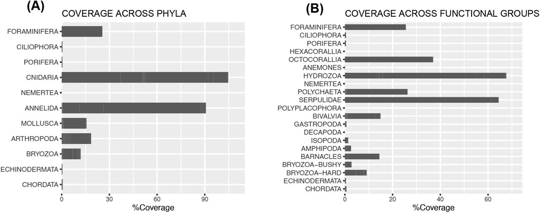
Figure 4. (A) Total coverage across the 11 Phyla. Cnidaria (Hydrozoa [13 species], Hexacorallia [4 sp.], Octocorallia [1 sp.]), and Annelida (polychaetes, c. 20 sp.) were the most abundant phyla with highest total coverage, followed by Foraminifera (one main species), Arthropoda (c. 13 sp.), Mollusca (22 sp.), and Bryozoa (11 sp.). Also represented, but in small numbers, were Ciliophora (represented by a single species, Folliculina viridis), Porifera (four species present), a few Nemertea, Echinodermata (4 sp. of brittle stars, juvenile sea stars and sea urchins), and Chordata (9 sp.). (B) Coverage across functional groups. Phyla was divided into different functional groups based on potential as secondary substrate (i.e., calcified or not). Cnidaria was divided into Hexacorallia (scleractinian corals, sessile), Anemones (mobile species), and Hydrozoa (bushy, sessile species). Annelida was divided into mobile or soft tubed polychaetes, and the sessile, calcifying Serpulidae family. Mollusca was divided into Polyplacophora (mobile), Bivalvia (mostly sessile saddle oysters, but incl. a few semi-sessile bivalves), and Gastropoda (mobile). Arthropoda was divided into larger mobile Decapoda (crabs), Isopoda (mobile), Amphipoda (both colonial semi-sessile, and free-living), and barnacles (sessile, calcifying). Bryozoa was divided into bushy bryozoans (Bryozoa-bushy), and encrusting, or erect calcified species (Bryozoa-hard). Serpulids, bivalves, barnacles, and bryozoans are calcifying organisms and potential substrates for coral larvae. The coverage and distribution of these groups could thus have a positive impact on later recruitment of corals.

The Cnidaria and Annelida (Polychaeta) were the most abundant groups, with 20 species of polychaetes, and cnidarians of three classes: Hydrozoa (13 species), Hexacorallia (3 anemones, 1 scleractinian, Caryophyllia smithii), and Octocorallia (1 species: Alcyonium digitatum). The most abundant species were two soft tube-dwelling polychaetes: the peacock worm Sabella pavonina (1060 individuals), and the similar but smaller Ampharete octocirrata (754 ind., Table 4). These were followed by three small crustaceans from the groups Amphipoda and Isopoda (AMP5, Janira maculosa, AMP4). The most abundant colonial organisms were the serpulid polychaete Filograna implexa (61% total coverage), and the hydrozoan Corydendrium dispar (39%). The remaining list of species was made up of more or less rare species, some only represented by a single individual. The Species Accumulation Curve shows that the curve is not yet levelling off despite the many replicates (200 panels in total, Figure 5A). A complete species list is found in the Supplementary Material (p 16–19). Species Rank-Abundance plots for species coverage (Figure 5B) and abundance (Figure 5C) data with species ranked by decreasing percentage coverage or individuals per species shows large drops between species at the higher end and more gradual decrease at the lower end. This was especially marked in abundances where there is a large drop from the two of the most abundant species (S. pavonina, A. octocirrata) to the following species.

Table 4

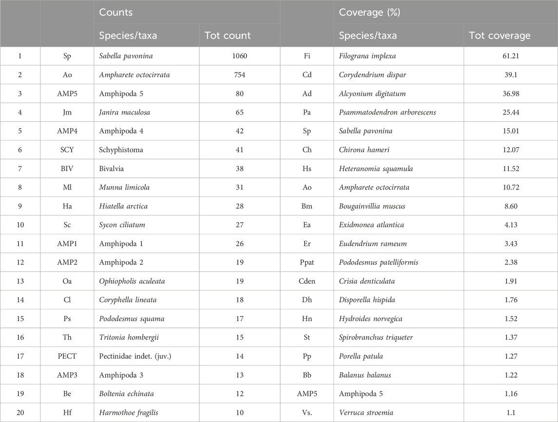
Table 4. Top 20 of species/taxa in counts data only on the left, and for total coverage data with both colonial and individuals included on the right. The two tube-dwelling polychaetes Sabella pavonina and Ampharete octocirrata were the most abundant species, followed by two amphipods and an isopod. A few clusters of Schyphistoma polyps of possibly Aurelia aurita gave a high total count. The species with the highest total coverage across all samples of panels were the colonial serpulid Filograna implexa, and the hydrozoan Corydendrium dispar. The soft octocoral Alcyonium digitatum were the most conspicuous colonial organism, with its large white and orange colonies, and on third place concerning per cent coverage. The bushy foraminiferan Psammatodendron arborescens was almost omnipresent. The amphipods could not be identified to species level, however, most seemed to belong to the genus Metopa or similar. They were numbered according to defining characters or association with host for the tube forming colonial amphipods (host either Sabella pavonina or large hydroid). A full species list is available in the Supplementary Material.

Figure 5

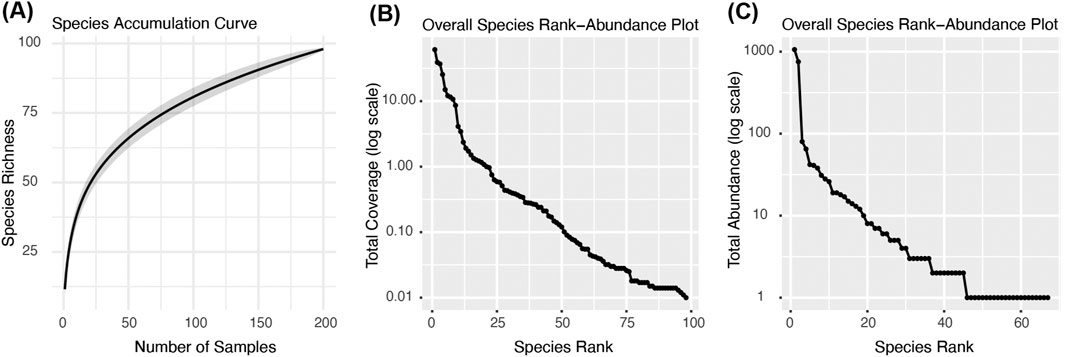
Figure 5. (A) Species Accumulation Curve for the entire dataset. There is no sign of levelling out. There were many rare species with very low abundances. (B) Species Rank-Abundance plot for coverage data showing the spread of values from the highest coverage to species with the lowest coverage ranked by decreasing level of coverage. (C) Species Rank-Abundance plot for abundance data showing the total number of individuals per species ranked by decreasing number of individuals. The two most abundant polychaetes at the top (Sabella pavonina and Ampharete octocirrata), and then a large drop to the amphipod (AMP5) and isopod Janira maculosa. Below there is a more gradual decrease in individuals per species.

Functional groups

To be able to separate out the species that potentially could be used as substrate for coral larvae, i.e., calcifying organisms, the Phyla were further divided into functional groups (Figure 4B). The Annelida was divided into mobile and soft-tubed polychaetes in one group, and the calcifying family Serpulidae in a separate group. The Arthropoda was divided into the mobile groups Decapoda, Isopoda, Amphipoda, and the sessile calcifying barnacles (Cirripedia). Bryozoa was likewise divided into “Bryozoa-bushy” and the encrusting or branching hard bryozoans, “Bryozoa-hard”. The Cnidaria was divided into three groups depending on their different functions: the scleractinian corals (Hexacorallia, only one individual of the cup coral C. smithii), the mobile anemones, and the soft octocorals (A. digitatum). Within Cnidaria only the presence of scleractinians could provide substrate for coral larvae. The total coverage of the groups that have the potential to function as secondary substrates were 64% for the serpulids, 15% for barnacles, and 9% for bryozoans (Figure 4B; Supplementary Table S4).

Species distribution across factors and Indicator Species Analysis

A detailed visualization of species distribution across all levels of the different factors were undertaken for the colonial and sessile species in heatmaps (Figures 6, 7). Overlayed on the heatmaps are the results from the Indicator Species Analysis (ISA). Species that had a significantly higher coverage or abundance on specific mixes, surfaces, sides, or rows (level above seafloor) are marked with green rectangles and the significance levels are indicated by asterisks (*** = 0.001; ** = 0.01; * = 0.05).

Figure 6

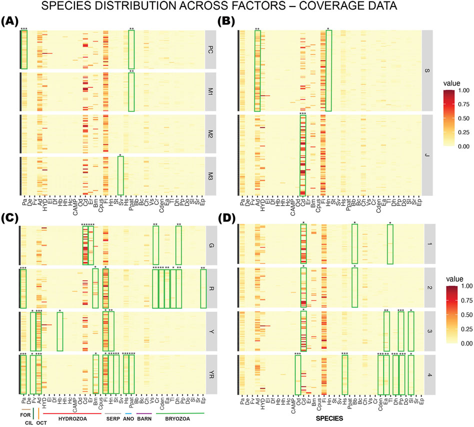
Figure 6. Faceted Heatmaps with species distribution across factors: (A) mix, (B) surface, (C) side, and (D) row (level above seafloor) for sessile species quantified by coverage data. Phyla are indicated by the colored lines on the bottom left panel: FOR = Foraminifera; CIL = Ciliophora; OCT = Octocorallia; Hydrozoa; SERP = Serpulidae; ANO = Anomiidae; BARN = Barnacles; Bryozoa. Overlayed are the Indicator Species Analysis with species that had significantly higher coverage on specific mixes, surfaces, sides, or rows, marked with green rectangles and significance levels given by asterisks (*** = 0.001; ** = 0.01; * = 0.05). Serpulids, anomiids, barnacles, and bryozoans are calcifying organisms and potential substrates for coral larvae. The distribution of these groups could thus have a positive impact on later recruitment of corals. G = southwest; R = northeast; Y = northwest; YR = southeast.

Figure 7

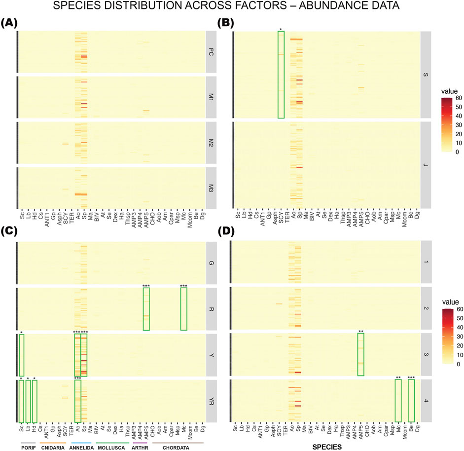
Figure 7. Faceted Heatmaps with species distribution across factors: (A) mix, (B) surface, (C) side, and (D) row (level above seafloor) for abundance data on sessile species. Phyla are indicated by the colored lines on the bottom left panel: PORIF = Porifera; Cnidaria; Annelida; Mollusca; ARTHR = Arthropoda; Chordata. Overlayed are the Indicator Species Analysis with species that had significantly higher coverage on specific mixes, surfaces, sides or rows, marked with green rectangles and significance levels given by asterisks (*** = 0.001; ** = 0.01; * = 0.05). The abundance of the two polychaetes Ampharete octocirrata (Ao) and Sabella pavonina (Sp) were so high that the lines for all other species are barely visible.

Coverage across factors

For mixes and surfaces in the two top panels in Figure 6A there were only three species that had significantly higher coverage on any of the substrates. On the PC controls the foraminiferan Psammatodendron arborescens (Pa) had significantly higher coverage than on the other mixes (p = 0.0003). Pododesmus patelliformis (Ppat, Anomiidae) had significantly higher coverage on PC and M1 (p = 0.0073). The serpulid Serpula vermicularis (Sv) had higher coverage on the M3 panels (p = 0.0313) but were in general one of the least abundant of the serpulids.

On panels with the higher complexity (slag) the soft octocoral A. digitatum (Ad, p = 0.0042) and serpulid Hydroides norvegica (Hn, p = 0.0469) had higher coverage (Figure 6B). On the jute panels the hydrozoan C. dispar (Cd) had significantly higher coverage (p = 0.0001). The colonial serpulid Filograna implexa (Fi) was close to significantly higher in coverage on jute (p = 0.0588) but was omnipresent and had an overall high coverage.

Local hydrodynamics and level above seafloor (row) had a more pronounced effect on species distribution, as seen on the two bottom panels for side (18 species affected) and row (9 species affected, Figures 6C,D). The larger hydrozoans, C. dispar (Cd) and Eudendrium rameum (Er) had significantly higher coverage on the southwest facing side (G), while bryozoans were gathering on the northeast facing side (R). For the other groups of species, the pattern was less distinct, and they were spread over the opposing sides facing northwest and southeast, having significantly higher coverage on two or three sides.

When it comes to level above seafloor (Figure 6D), the bryozoans seemed to prefer the lower levels closer to the seafloor (row 3, 4), except Tubulipora liliacea (Tl, bryozoa), as well as the barnacle Balanus balanus (Bb) that preferred the higher level. The hydrozoan C. dispar (Cd) was less abundant only on the lowest level, while equally high coverage was found on the top three levels. The rare hydrozoan Obelia dichotoma (Od) had significantly higher coverage on the lowest level.

Abundance across factors

Detailed visualizations with heatmaps were also made for abundance data with 30 species of sessile and semi-sessile organisms (Figures 7A–D). Only the species that are mainly sessile were kept for this analysis. The highly mobile bivalve family Pectinidae and free-living amphipods were removed, as well as gastropods and free-living polychaetes. Tube-dwelling polychaetes, colonial amphipods, and anemones are included since they are mostly sessile. No species was significantly more abundant on any of the concrete mixes (Figure 7A).

For surface complexity it was only the Schyphistoma (hydrozoan polyps) that was significantly more abundant on slag (p = 0.0243, Figure 7B). For side one of the tube-building amphipods (AMP5) and chordate (Mc, Molgula citrina) were significantly more abundant on the northeast facing side (R, Figure 7C). The most abundant polychaete, S. pavonina (Sp) was more abundant on the northwest side (Y, p = 0.0002), while A. octocirrata (Ao, p = 0.0001) was significantly more abundant on the opposing yellow (Y) and yellow+red (YR) sides, facing northwest and southeast, respectively. The very high abundances of these species make the low-abundance species hard to detect in the heatmaps as most other species had very low counts. Poriferans were found to gather on the southeast facing side (YR). There were 3 species that preferred to be closer to the seafloor on row 3–4, the tube-building amphipod (AMP5) and two chordates, M. citrina (Mc) and Boltenia echinata (Be, Figure 7D).

Diversity indices across factors

Four Diversity Indices (DI) were calculated for all identified or defined species from per cent coverage data: Shannon-Wiener Diversity Index (H′), Simpson, species Richness, and Evenness (Table 5; Figure 8). The overall diversity in the material was high, with a Shannon-Wiener Index of 1.78 ± 0.35 (mean ± SD), ranging between 0.7 and 2.5. Species richness was 11.5 ± 2.96 (mean ± SD), with a minimum of 4, and a maximum of 20 species present on one sample. Evenness was relatively high (0.73 ± 0.10, mean ± SD). Simpson’s Index and Evenness were not included in the statistical analyses, but values are given in Table 5, both overall for the entire dataset, and values across the different factors (mix, surf, side, row).

Table 5

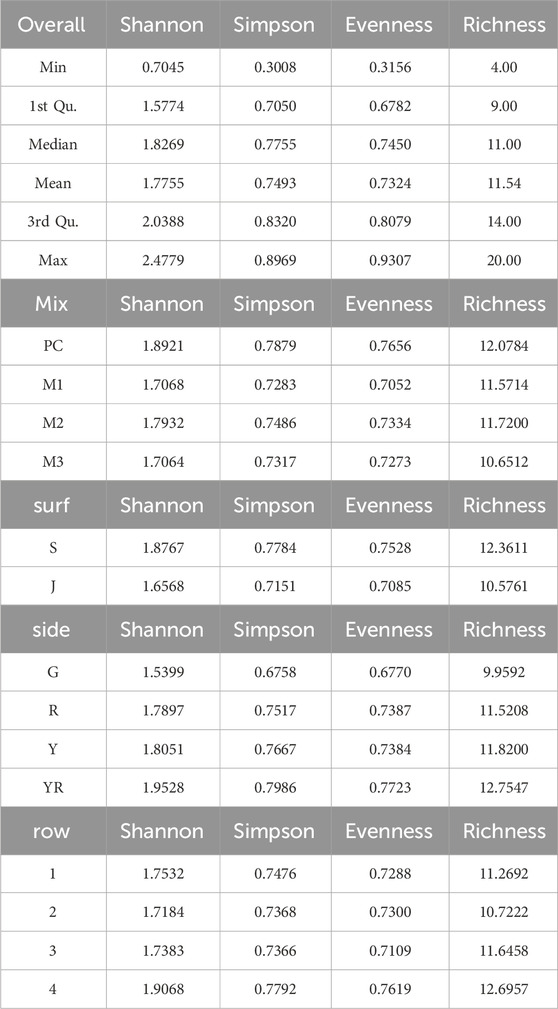
Table 5. Diversity Indices: the overall DI for the entire dataset; and mean DI across the different factors: mix, surface, side, and row.

Figure 8

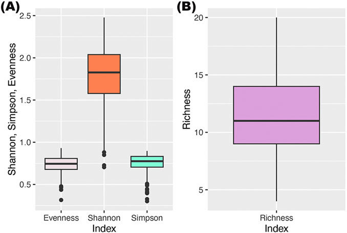
Figure 8. Diversity Indices for the entire dataset. (A) Evenness (0.73 ± 0.10, mean ± SD), Shannon-Wiener Diversity Index (1.78 ± 0.35, mean ± SD), and Simpson (0.75 ± 0.11, mean ± SD). (B) Species Richness (11.54 ± 2.96, mean ± SD). The maximum richness for one sample was 20 species. Abundance data was recalculated to coverage to include all species.

Multifactorial ANOVAs

Total coverage

The overall frequency distribution of the entire dataset for total coverage was not skewed (skewness 0.3067), however, a mild left-skew was found in the data for M3 (−0.044), side G (−0.195), and rows 1 (−0.0681) and 4 (−0.0846). The skewness was barely visible in the histograms (Supplementary Figure S7). A Bartlett’s test of homogeneity came out significant for factor mix (K² = 8.5152, df = 3, p-value = 0.03648). The rest of the factors had homogenous variances. The residuals vs. fitted had only minor deviations and observations aligned well in the Q-Q plots, and there were no extreme values that had an undue effect on the data in Residuals vs. leverage (Supplementary Figures S9, S10). These minor deviations from normality and homogeneity in variances were deemed too small to prompt action.

The total coverage of fauna differed across mixes (F(3,186) = 6.748, p = 0.000241), with the highest overall coverage on the controls (PC) and dropping over the three mixes (Figure 9A; Table 6). A Tukey HSD post hoc test gave significant results only between PC vs. M3 (p = 0.0002094). The difference between surfaces within mix was non-significant and coverage could be higher or lower on one surface compared to the other. Note that the expression mix:surf in this case is not an interaction, but defines surf as nested under mix, since surface is represented within each mix instead of analyzed as a standalone factor.

Figure 9

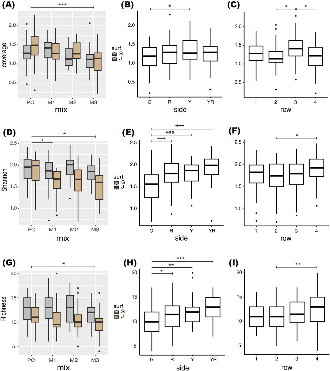
Figure 9. Results from the multifactorial ANOVAs: (A) Differences between mix and surf, with surf nested under mix for coverage. There was a significant difference in coverage between mixes (F(3, 186) = 6.748, p = 0.000241), and a Tukey HSD gave a significant difference between PC and M3 (p = 0.0002094). The differences between surface within mix was non-significant. (B) Difference in coverage across sides. There was a significant difference between sides (F(3, 186) = 3.386, p = 0.01928). A Tukey HSD gave significant differences between G and Y (p = 0.009318). (C) The difference in coverage across rows (level above seafloor) was significant (F(3, 186) = 3.709, p = 0.012651). A Tukey HSD gave significant differences between 3 and 2 (p = 0.0201978), and 3 and 4 (p = 0.0258531). (D) The difference between surfaces within mix was significant (F(4, 186) = 6.225, p = 0.000101) for the Shannon-Wiener Diversity Index (H′) with lower values of H′ on jute than slag for all mixes but not within PC. (E) The difference in H′ across sides was highly significant (F(3, 186) = 17.610, p = 4.18⁻¹⁰). A Tukey HSD gave significant differences between G vs. R (p = 0.0001424), G vs. Y (p = 0.0000539), and G vs. YR (p = 0.0000). (F) The difference in H′ across rows (level above seafloor) was significant (F(3, 186) = 3.569, p = 0.015196). A Tukey HSD gave significant differences between 4 and 2 (p = 0.0114716). (G) The differences between surfaces within mix was significant (F(4, 186) = 5.353, p = 0.000421) with species richness being lower on jute than slag for all mixes including PC. (H) The difference in species richness across sides was highly significant (F(3, 186) = 10.645, p = 1.72⁻⁰⁶). A Tukey HSD gave significant differences between G vs. R (p = 0.0108309), G vs. Y (p = 0.0017687), and G vs. YR (p = 0.0000006). (I) The difference in species richness across rows was significant (F(3, 186) = 4.349, p = 0.005164). A Tukey HSD gave significant differences between row 4 vs. 2 (p = 0.0025818).

Table 6

Table 6. Results from Multifactorial ANOVAs for the three response variables: coverage; Shannon-Wiener diversity index (H′); and species richness. All factors are fixed. Note that mix:surf in this case is not an interaction but defines surface as nested under mix. Significant p-values indicated by bold numbers. df = degrees of freedom; SS = sum of squares; MS = mean of squares; F = F-statistic; P = p-value and significance level.

There was a significant difference in coverage between sides (F(3,186) = 3.386, p = 0.01928, Figure 9B). A Tukey HSD post hoc test gave significant results between G vs. Y (p = 0.009318). Coverage was also significantly different between rows (F(3,186) = 3.709, p = 0.012651), with significantly higher coverage on level 3, c. 60 cm above the seafloor, compared to level 2 (p = 0.0201978) and 4 (p = 0.0258531, Figure 9C).

Shannon-Wiener Diversity Index

The Shannon-Wiener DI (H′) data was slightly left-skewed (−0.752), with higher frequencies of higher diversity values (Supplementary Figure S11). A square root transformation was tested, however, this led to an over-transformation with data ending up being right-skewed. Q-Q plots revealed that PC and M2 fell within range. Only the frequency distribution of M1 (skewness: -0.89) and M3 (−0.79) had an excess left-skew and points outside the range in the Q-Q-plots. Since the weakest transformation was too much, we decided to run the analyses on the untransformed data.

A Bartlett’s test showed that surface (K² = 4.4165, df = 1, p = 0.03559) and side (K² = 12.403, df = 3, p = 0.006124) had significant differences in variances between treatments while mix and row had homogenous variances.

The difference between slag vs. jute within mix (mix:surf) was significant (F(4, 186) = 6.225, p = 0.000101) with lower values of H′ on jute than slag for all mixes but not within PC (Figure 9D). The difference in H′ across sides was highly significant (F(3, 186) = 17.610, p = 4.18⁻¹⁰) indicating that local hydrodynamics had a stronger influence on diversity than substrate composition or complexity (Figure 9E). A Tukey HSD gave significant differences between G vs. R (p = 0.0001424), G vs. Y (p = 0.0000539), and G vs. YR (p = 0.0000). The difference in H′ across rows (level above seafloor) was significant (F(3, 186) = 3.569, p = 0.015196) with the highest H′ associated with the level closest to the seafloor (row 4, 15 cm above) as revealed by a Tukey HSD (row 4 vs. 2, p = 0.0114716, Figure 9F).

Species richness

The Species Richness data were all normally distributed, had no skewness and variances were homogenous.

The difference between surfaces within mix was significant (F(4, 186) = 5.353, p = 0.000421) for the species richness, with lower values of richness on jute than slag for all mixes including PC, indicating that level of complexity had a large effect on species richness (Figure 9G). There was also a significant difference between PC vs. M3 (p = 0.0421714) according to the Tukey HSD. This effect was, however, weaker than the difference between surfaces within mix. The difference in species richness across sides was highly significant (F(3, 186) = 10.645, p = 1.72⁻⁰⁶, Figure 9H). A Tukey HSD gave significant differences between G vs. R (p = 0.0108309), G vs. Y (p = 0.0017687), and G vs. YR (p = 0.0000006). The difference in species richness across rows was significant (F(3, 186) = 4.349, p = 0.005164). A Tukey HSD gave significant differences between row 4 vs. 2 (p = 0.0025818, Figure 9I).

Discussion

The aim of the present study was to find the optimal mix of concrete to use for the production of artificial reefs (ARs) within the LIFE Lophelia cold-water coral reef habitat restoration project in the Skagerrak. The goal was to find a material composition that assures longevity of ARs, reduces the carbon footprint, and enhances recruitment of Desmophyllum pertusum and reef associated fauna. The main findings of this study were that the benthic invertebrates associated to the reef habitat were more affected by surface complexity and orientation than by the material composition. There were no D. pertusum recruits observed on the panels. The lack of coral recruits in this field study could indicate that larvae were not available during the deployment period, and that coral recruitment does not occur on a yearly basis.

Effect of mix

The mineral composition of the panels (mix) had a minor effect on coverage and diversity indices. The M3 mix had overall the poorest outcome while the mixes M1 and M2 were more similar to standard Portland cement panels (PC). There were significantly lower values on panels with the M3 mix compared to PC throughout all response variables (coverage, Shannon-Wiener diversity [H’], richness), and in addition there was a significantly lower H′ on M1 panels compared to PC. Adding additional silica oxide on top of what already is present in the GGBFS appears to be of little value and lowering of pH had no positive effects on faunal recruitment. In shallow water, tiles with a pH of 9–10.5 have been shown to increase recruitment compared to standard Portland cement tiles with a pH of 12.5–13.5 (Perkol-Finkel and Sella, 2014). These previous field trials were done in the Red Sea and Mediterranean at 6–10 m depth. The slower recruitment rate in the deep-sea environment may allow time for pH of the concrete to reach equilibrium with the seawater pH before major recruitment starts. It is also found that algae might be the group that is benefitting the most from a lower pH while calcifying fauna such as barnacles prefer panels with higher pH (Guilbeau et al., 2003). Most fauna associated with D. pertusum reefs thrives on the dead parts of the reefs, high in aragonite, and are thus adapted to live on substrates rich in calcium carbonate. There were no observed D. pertusum recruits on the panels in the present study, however, in a companion paper to this field study, we investigated larval settling of D. pertusum in a laboratory setting (Strömberg et al., 2025, in this issue). These laboratory trials showed that larvae preferred the M3 mix. So, there is a potential of benefiting coral larvae before the associated fauna by using the high silica mix for the entire AR or by adding parts to the main AR with a higher silica content and lower pH for the coral larvae. Adding too much silica could, however, compromise the durability of the concrete, and adding smaller parts made from the M3 mix on top of a larger AR with lower silica content would be recommendable.

Effect of surface complexity

A clear effect of surface complexity was seen on the diversity indices (Figures 9D,G). The more complex surface with slag had higher H′ and richness, while surface complexity had no significant effect on coverage (Table 6). The only significant effect was found in species richness between slag and jute on the M1 panels (M1:J vs. M1:S, p = 0.0349752). The hydroid Corydendrium dispar was the sole species contributing to higher coverage on the jute panels, as seen in the heatmap (Figure 6B), indicating a somewhat simplified fauna on the less complex surfaces. Recruitment in Hydroids benefits from edge effects and they commonly recruit along edges, and subsequently use stolon to spread across a substrate and can rapidly colonize adjacent surfaces. This can give them an advantage over other fauna on less complex surfaces. Macro- and microscale substrate complexity and rugosity has been found to increase biodiversity in several studies (e.g., Spieler et al., 2001; Sella and Perkol-Finkel, 2015; Loke and Todd, 2016; Sedano et al., 2020). This is in line also with a recent review where it was found that surface roughness was more important for recruitment than the chemical composition of the substrates, although the inclusion of slag cement (GGBFS) was also found to be beneficial (Hayek et al., 2023). During documentation many mobile polychaetes and isopods were observed using the crevices between the pieces of slag for refuge. These species are probably underestimated since they were difficult to detect, however, they still contributed to the higher values on the complex surfaces with slag.

The loss of the jute cloth is confounding the results somewhat and is a weakness in this study. The aim was to test two different types of complex surfaces, not to test a high vs. lower complexity surface as was the result with the loss of cloth. The timeline is unknown, i.e., how long it took for the cloth to detach, and how much settling had already occurred at the time. Hopefully the cloth detached soon after deployment, and had little effect on the recruitment that followed, but we cannot know how big effect this had on the results. The long deployment time of 19 months has hopefully minimized this effect. If we were to repeat this experiment again, it would be interesting to compare the complex surface with slag to panels with completely smooth surfaces, and adding an intermediate complexity panel with ridges or a simplified texture to see how the level of complexity affects the outcomes. The results are, however, in line with previous literature. Loke and Todd (2016) tested different levels of complexity and found a linear increase in species richness with increasing complexity while controlling for surface area. Species richness was also found to be higher in association with pits than with grooves, towers, or darts (jagged edges). Most species preferred a pit-size in close fit to their own body size. This was also found in a study by Whalan et al. (2015) in a settling experiment with coral larvae. Larvae preferred settling in pits fitting the planula width. In many previous trials with artificial reefs or settling panels, the conclusion has often been the higher the complexity, the higher the diversity (e.g., Clark and Edwards, 1994; Sherman et al., 2002). The ‘complexity’ has, however, usually been at a larger scale than the fine-scale complexity used in Loke and Todd (2016) or in this study.

Effect of orientation

Local hydrodynamics and orientation of the side the panels were mounted on had a large effect on both Shannon-Wiener diversity index (H′) and species richness, but less so on coverage. The southeast facing side (YR) had the highest values. The highest current speeds were heading southeast, directly hitting the Y side, while currents heading in the opposite direction (northwest) were more often in the 10–20 cm s^-1 range (Nestorowicz et al., 2025). Since the coral mound with live and dead coral reefs were situated northwest of the rack most locally recruiting larvae may have come with the faster southeast-heading currents. The bars of the rack at the northwest side (Y) of the rack could thus act as a current breaker, causing micro eddies that assisted the larvae in attaching as they reached the YR side. Both Y and YR had higher H′ and richness, while the two sides that took the currents along the sides had lower values, although side R (facing northeast) had intermediate values, and G (facing southwest) had the lowest values. If this is an effect of where the source populations were situated in relation to the sides of the rack, or an effect of the current directions is hard to tease out. The rack was not in perfect position with any side facing the current directions head on, although the rack was moved by the currents to have side Y and YR facing the currents closer to head on by the end. The experimental design with only one rack with four sides cannot fully resolve the effect of hydrodynamics and current directions, however, it shows that other factors have a stronger effect on recruitment than the material composition. Orientation was a secondary factor, while mix, complexity, and level above seafloor were the main factors of interest, so the experimental design was made accordingly.

Effect of level above seafloor

The effect of level above seafloor (row) had less of an effect than anticipated, however, the lower levels had significantly higher values of all response variables (coverage, H′, richness), with coverage being highest on row 3 (c. 30 cm above seafloor) and H′ and richness higher on row 4, c. 15 cm above seafloor. This was especially true for the coverage of bryozoans (Figure 6D) and abundance of two of the chordates (Figure 7D) that had significantly higher numbers on the lower levels above seafloor (row 4 and 3). The difference between levels was confounded by the fact that the panels could not be mounted on the same level on each bar, so the mid-levels were overlapping. A difference should be detectable, however, between the top and bottom most rows if there had been one. The reef associated fauna in general seems to recruit equally well within 15 and 75 cm above seafloor, except for bryozoans and certain chordates. Larvae of D. pertusum is expected to prefer higher elevation to get into more favorable current speed, however, the single individual of a scleractinian coral found on the panels, Caryophyllia smithii, was found on row 3 at c. 30 cm above seafloor (side YR). At this site the current speed is, however, so high that even the seafloor is current swept and kept free of sediments. At sites with lower current speeds and high sedimentation rates there could be a different outcome. The anemones and Scyphistoma polyps had no detectable preferences. The soft octocoral Alcyonium digitatum had higher abundances on the Y and YR sides, and on the more complex surface (slag), but no preferences when it came to level above seafloor. Reef associated fauna will usually be most abundant at the dead parts at the base of the reef, with only moderate elevation needed, while coral larvae need higher elevation, so these results are in line with natural occurrences.

Distribution and coverage of potential secondary substrates

The calcifying organisms that could constitute a possible substrate for D. pertusum larvae did not show any preferences for level above seafloor, except for the barnacle Balanus balanus that preferred higher elevation (Figure 6D). The largest barnacle, Chirona hameri, had no preference and were well spread across all levels. This is probably the most likely candidate to serve as substrate for D. pertusum larvae. In total, barnacles had a coverage of 15%, thus providing ample substrate for coral larvae. Young D. pertusum colonies have been found on deep-sea barnacles in a previous study (Strong et al., 2023). Populations of C. hameri seems to have been fluctuating over the last decades. They were not found in a survey in 1999 despite being common before 1995 (Lundälv and Jonsson, 2000). Increased sedimentation seemed to be the cause of their demise at the time, and the renewed presence of the species on these panels could be an indication that environmental conditions has improved. It is possible that the restrictions in trawling implemented in 2001 has helped.

The serpulid polychaetes had higher coverage on the YR side but no preference of level. The colonial serpulid Filograna implexa creates an intricate matrix of interconnected tubes that may well cause other larvae to precipitate within the matrix. It is, however, a weak structure to use as a substrate for D. pertusum. The solitary serpulids with well attached tubes are more likely to be a good substrate. The coverage of serpulids in total was very high (64%), however, this was mainly due to the F. implexa colonies. The bivalves are unlikely as substrates for coral larvae since they are semi-mobile. Only the attached bottom shell of the saddle oysters (Anomiidae) could potentially be suitable once the oyster has died and lost the hinged top shell. One species, Heteranomia squamula, had significantly higher coverage on the lowest level above seafloor but were present at all levels. Saddle oysters are very common in this area; however, they are often seen growing on smooth boulders and rock faces with higher sediment loads where no new coral recruits have been observed. The hard bryozoans had a coverage of merely 9%; however, some species have a very robust build with small orifices that could provide a solid substrate for coral larvae. Many other organisms use the orifices of dead bryozoan colonies for shelter (personal observation).

Associated fauna

Jensen and Frederiksen (1992) examined the associated fauna of 25 blocks of L. pertusa from the Faroe shelf and found 256 species from 18 Phyla. The most abundant and species rich group was the polychaetes, followed by bivalves, echinoderms, brachiopods, and crustaceans. Bryozoans and poriferans had many observed species but no quantification was done. The resolution of their study was high and included protozoans (15 species) and nematodes (9 species). The overall diversity in their material was at H′ 5.50, despite that colonial organisms (91 species) were excluded, using only abundance data on individuals. In their material there were 13 species that had counts in the hundreds, while a majority was represented by 10 or less individuals. In our material only two species were very abundant, several hundreds to thousands, while 9 species had higher than 20 counts, another 9 species between 10 and 19, and the remaining had single digit numbers. Four species dominated in coverage, F. implexa (serpulid), C. dispar (hydrozoa), A. digitatum (octocoral), and P. arborescence (foraminifera).

Hydrozoans are less abundant and have smaller less developed colonies in the Faroes than in Norway and Sweden and made up a smaller part of the fauna in their material. Otherwise, there is a good overlap in phyla composition. In the present material Cnidaria was the largest group, mainly comprised of hydrozoans, but also the octocoral A. digitatum. The polychaetes (Annelida) made up the second largest group with 20 species present. The brittle stars (Ophiuorida) are very common in D. pertusum habitats, and many were found on the panels even though most were observed dropping off the rack as soon as it was hauled out of the water. Especially Ophiopholis aculeata that hides in crevices, just protruding their arms, were still on the panels. What is missing in our material are the brachiopods, a group that is highly associated with CWC habitats and has been common in the area. Likewise, we found no species on the panels that are obligate on D. pertusum, such as the polychaete Eunice norvegica, or the squat lobster Munidopsis serricornis.

Noteworthy was the presence of two species on the panels that never have been reported for the Skagerrak before, the anemone Actinothoe sphyrodeta (single specimen), and the tube-dwelling polychaete Myxicola aesthetica (two specimens). The anemone is common around the British Isles, with some occurrences in the North Sea, often associated with kelp (Hansson, 2011; Rodríguez et al., 2025, WoRMs). The distribution is similar for M. aesthetica (Read and Fauchald, 2025, WoRMs). These are species with distinct characters, not easily confused with other species, although the small size of M. aesthetica and being enveloped within a mucus-like tube makes it harder to detect and identify. No dissection of the animal within the tube was made.

Conclusion

In conclusion, the standard Portland cement (PC) controls and mix 1 and 2 (M1, M2) with the more complex surface (slag) were equal in both Shannon DI and Species Richness, while mix 3 (M3) were lower in both variables, especially with the less complex surface jute on top. A higher complexity of the surface lead to a higher diversity and richness of the recruited fauna, congruent with the results of previous studies on benthic recruitment. The reef associated fauna is less selective than D. pertusum larvae when it comes to substrate composition (Strömberg et al., 2025, in this issue), and more affected by surface complexity and local hydrodynamics. Some species also have preferences when it comes to elevation above seafloor, with some preferring to be closer to the seafloor, while others prefer higher current speeds at greater elevation. This can be useful information if you want to target specific species or groups in a restoration project.

With material composition (mix) being of minor importance for the reef associated fauna, one can focus on the best mix considering longevity of ARs and lowest carbon footprint. With a 50:50 mix of PC and GGBFS having been reported to have the highest compressive strength (Osmanovic et al., 2018) and the Dutch recommended standard having a GGBFS content of up to 72% (Polder et al., 2014; Gulikers, 2016) this could provide a good guidance regarding the optimal range as being 50%–70% GGBFS for the longevity aspect. And the higher the GGBFS content the lower the carbon footprint will be (Song and Saraswathy, 2006).

Data availability statement

The authors acknowledge that the data presented in this study must be deposited and made publicly available in an acceptable repository, prior to publication. Frontiers cannot accept a manuscript that does not adhere to our open data policies. The dataset is available via SND, the Swedish National Data service at https://doi.org/10.5878/7fmy-j376.

Ethics statement

The manuscript presents research on animals that do not require ethical approval for their study.

Author contributions

SS: Conceptualization, Data curation, Formal Analysis, Funding acquisition, Investigation, Methodology, Software, Validation, Visualization, Writing – original draft. AL: Funding acquisition, Methodology, Project administration, Software, Writing – review and editing.

Funding

The author(s) declare that financial support was received for the research and/or publication of this article. This study was part of the project LIFE Lophelia, LIFE18 NAT/SE/000959, funded by the EU LIFE fund Nature and Biodiversity and co-financed by the Swedish Agency for Marine and Water SWAM co-financing dairy number 208-19. The project was led by the County Administrative Board of Västra Götaland, and all research within the project was conducted by SS and AL at University of Gothenburg, Department of Marine Sciences, Tjärnö Marine Laboratory, with both CABO and UGOT contributing with funding via salaries.

Acknowledgments

A big thank you to our internship student Josefin Lindell who helped mounting the many panels on the rack. We are also grateful to Björn Haase at Höganäs AB, Sweden, for contributing with metallurgic slag, and to the concrete laboratory of Thomas Betong AB, C-lab, for the help with deciding on the concrete mixes and testing pH and compressive strength. And we are always grateful to our ROV pilots Joel White, Roger Johannesson, and Gunnar Cervin for helping with deployments and retrievals of equipment, in this case a big heavy rack. Many thanks also to our skippers on R/V Nereus, Peter Nilsson and Linus Andersson.

Conflict of interest

The authors declare that the research was conducted in the absence of any commercial or financial relationships that could be construed as a potential conflict of interest.

Generative AI statement

The author(s) declare that Generative AI was used in the creation of this manuscript. Chat GPT was used for customizing R code.

Any alternative text (alt text) provided alongside figures in this article has been generated by Frontiers with the support of artificial intelligence and reasonable efforts have been made to ensure accuracy, including review by the authors wherever possible. If you identify any issues, please contact us.

Publisher’s note

All claims expressed in this article are solely those of the authors and do not necessarily represent those of their affiliated organizations, or those of the publisher, the editors and the reviewers. Any product that may be evaluated in this article, or claim that may be made by its manufacturer, is not guaranteed or endorsed by the publisher.

Supplementary material

The Supplementary Material for this article can be found online at: https://www.frontiersin.org/articles/10.3389/fenvs.2025.1561412/full#supplementary-material

References

Bhat, A. V., and Tengli, S. K. (2019). Behaviour of ground granulated blast furnace slag concrete in marine environment under chloride attack. Int. J. Innov. Technol. Explor. Eng. 9 (1), 278–302. doi:10.35940/IJITEE.A4699.119119

CrossRef Full Text | Google Scholar

Bourque, J., and Demopoulos, A. (2018). The influence of different deep-sea coral habitats on sediment macrofaunal community structure and function. PeerJ 6, e5276. doi:10.7717/peerj.5276

PubMed Abstract | CrossRef Full Text | Google Scholar

Buhl-Mortensen, L., Vanreusel, A., Gooday, A. J., Levin, L. A., Priede, I. G., Buhl-Mortensen, P., et al. (2010). Biological structures as a source of habitat heterogeneity and biodiversity on the deep ocean margins. Mar. Ecol. 31 (1), 21–50. doi:10.1111/j.1439-0485.2010.00359.x

CrossRef Full Text | Google Scholar

Büscher, J. V., Wisshak, M., Form, A. U., Titschack, J., Nachtigall, K., and Riebesell, U. (2019). In situ growth and bioerosion rates of Lophelia pertusa in a Norwegian fjord and open shelf cold-water coral habitat. PeerJ 7, e7586. doi:10.7717/peerj.7586

PubMed Abstract | CrossRef Full Text | Google Scholar

Clark, S., and Edwards, A. J. (1994). Use of artificial reef structures to rehabilitate reef flats degraded by coral mining in the Maldives. Bull. Mar. Sci. University of Miami - Rosenstiel School of Marine, Atmospheric & Earth Science. 55 (2-3), 724–744. Available online at: https://www.ingentaconnect.com/contentone/umrsmas/bullmar/1994/00000055/f0020002/art00038

Google Scholar

Convention on Biological Diversity (CBD) (2025). Resolution 65/161: COP 10 decision X/2. Strategic Plan for biodiversity 2011–2020. New York, NY: Aichi Biodiversity Targets. Available online at: https://www.cbd.int/sp/targets (Accessed December 2024).

Google Scholar

Douarin, M., Sinclair, D. J., Elliot, M., Henry, L.-A., Long, D., Mitchison, F., et al. (2014). Changes in fossil assemblage in sediment cores from mingulay reef complex (NE Atlantic): implications for coral reef build-up. Deep Sea Res. Part II Top. Stud. Oceanogr. 99, 286–296. doi:10.1016/j.dsr2.2013.07.022

CrossRef Full Text | Google Scholar

Fosså, J. H., Mortensen, P., and Furevik, D. M. (2002). The deep-water coral Lophelia pertusa in Norwegian waters: distribution and fishery impacts. Hydrobiologia 471 (1-3), 1–12. doi:10.1023/a:1016504430684

CrossRef Full Text | Google Scholar

Frank, N., Freiwald, A., Correa, M. L., Wienberg, C., Eisele, M., Hebbeln, D., et al. (2011). Northeastern Atlantic cold-water coral reefs and climate. Geology 39 (8), 743–746. doi:10.1130/g31825.1

CrossRef Full Text | Google Scholar

Gannon, P., Seyoum-Edjigu, E., Cooper, D., Sandwith, T., Ferreira de Souza Dias, B., Paşca Palmer, C., et al. (2017). Status and prospects for achieving Aichi biodiversity target 11: implications of national commitments and priority actions. Parks 23 (2), 13–26. doi:10.2305/iucn.ch.2017.parks-23-2pg.en

CrossRef Full Text | Google Scholar

Gilmour, J. (1999). Experimental investigation into the effects of suspended sediment on fertilisation, larval survival and settlement in a scleractinian coral. Mar. Biol. 135, 451–462. doi:10.1007/s002270050645

CrossRef Full Text | Google Scholar

Guilbeau, B. P., Harry, F. P., Gambrell, R. P., Knopf, F. C., and Dooley, K. M. (2003). Algae attachment on carbonated cements in fresh and brackish Waters—preliminary results. Ecol. Eng. 20 (4), 309–319. doi:10.1016/s0925-8574(03)00026-0

CrossRef Full Text | Google Scholar

Gulikers, J. (2016). Coastal protection structures in the Netherlands. Mar. Concr. Struct., 321–337. doi:10.1016/b978-0-08-100081-6.00012-x

CrossRef Full Text | Google Scholar

Hansson, H. G. (2011). Marina Syd-Skandinaviska evertebrater – ett naturhistoriskt urval. Available online at: https://www.gu.se/sites/default/files/2020-10/Hansson%202011.pdf. (Accessed December 2024)

Google Scholar

Hayek, M., Salgues, M., Souche, J.-C., De Weerdt, K., and Pioch, S. (2023). How to improve the bioreceptivity of concrete infrastructure used in marine ecosystems? Literature review for mechanisms, key factors, and colonization effects. J. Coast. Res. 39 (3), 553–568. doi:10.2112/jcoastres-d-21-00158.1

CrossRef Full Text | Google Scholar

Henderson, M. J., Huff, D. D., and Yoklavich, M. M. (2020). Deep-sea coral and sponge taxa increase demersal fish diversity and the probability of fish presence. Front. Mar. Sci. 7, 593844. doi:10.3389/fmars.2020.593844

CrossRef Full Text | Google Scholar

Henry, L.-A., Frank, N., Hebbeln, D., Wienberg, C., Robinson, L., van de Flierdt, T., et al. (2014). Global ocean conveyor lowers extinction risk in the deep sea. Deep Sea Res. Part I Oceanogr. Res. Pap. 88, 8–16. doi:10.1016/j.dsr.2014.03.004

CrossRef Full Text | Google Scholar

Husebø, Å., Nøttestad, L., Fosså, J., Furevik, D., and Jørgensen, S. (2002). Distribution and abundance of fish in deep-sea coral habitats. Hydrobiologia 471, 91–99. doi:10.1023/a:1016549203368

CrossRef Full Text | Google Scholar

Huvenne, V. A. I., Bett, B. J., Masson, D. G., Le Bas, T. P., and Wheeler, A. J. (2016). Effectiveness of a deep-sea cold-water coral marine protected area, following eight years of fisheries closure. Biol. Conserv. 200, 60–69. doi:10.1016/j.biocon.2016.05.030

CrossRef Full Text | Google Scholar

Jackson, M. D., Oleson, J. P., Moon, J., Zhang, Y., Chen, H., and Gudmundsson, M. T. (2018). Extreme durability in ancient Roman concretes. Am. Ceram. Soc. Bull. 97 (5), 22–28.

Google Scholar

Jägerskiöld, L. A. (1971). A Survey of the Marine Benthonic Macro-Fauna along the Swedish West Coast 1921-1938. Acta Regiae Societatis Scientiarum et Litterarum Gothoburgensis. Zoologica (6), 146.

Google Scholar

Järnegren, J., and Kutti, T. (2014). “Lophelia pertusa in Norwegian waters,” in What have we learned since 2008? Norwegian Institute for Nature Research. Report 1028. 40.

Google Scholar

Jensen, A., and Frederiksen, R. (1992). The fauna associated with the bank-forming deepwater coral Lophelia pertusa (Scleractinaria) on the faroe shelf. Sarsia 77 (1), 53–69. doi:10.1080/00364827.1992.10413492

CrossRef Full Text | Google Scholar

Jones, C., Lawton, J., and Shachak, M. (1994). Organisms as ecosystem engineers. Oikos 69, 373–386. doi:10.2307/3545850

CrossRef Full Text | Google Scholar

Jonsson, L. (2014). Trålskyddsuppföljning i koster-väderöfjorden: ROV-undersökning av bottenfaunan. Rapport 15.

Google Scholar

Loke, L. H., and Todd, P. A. (2016). Structural complexity and component type increase intertidal biodiversity independently of area. Ecology 97 (2), 383–393. doi:10.1890/15-0257.1

PubMed Abstract | CrossRef Full Text | Google Scholar

Lundälv, T., and Jonsson, L. (2000). Inventering av Koster-Väderöområdet med ROV-teknik. En pilotstudie. Stockholm: Naturvårdsverket.

Google Scholar

Ly, O., Yoris-Nobile, A. I., Sebaibi, N., Blanco-Fernandez, E., Boutouil, M., Castro-Fresno, D., et al. (2021). Optimisation of 3D printed concrete for artificial reefs: biofouling and mechanical analysis. Constr. Build. Mater. 272, 121649. doi:10.1016/j.conbuildmat.2020.121649

CrossRef Full Text | Google Scholar

Maier, S. R., Brooke, S., De Clippele, L. H., de Froe, E., van der Kaaden, A. S., Kutti, T., et al. (2023). On the paradox of thriving cold-water coral reefs in the food-limited deep sea. Biol. Rev. 98 (5), 1768–1795. doi:10.1111/brv.12976

PubMed Abstract | CrossRef Full Text | Google Scholar

Moeller, M., Nietzer, S., Schils, T., and Schupp, P. J. (2017). Low sediment loads affect survival of coral recruits: the first weeks are crucial. Coral Reefs 36, 39–49. doi:10.1007/s00338-016-1513-1

CrossRef Full Text | Google Scholar

Nestorowicz, I.-M., Luckas, N., Fagerström, V., Strömberg, S. M., and Larsson, A. I. (2025). “Environmental variation in live and historical cold-water coral reefs,” in Skagerrak with implications for restoration.

Google Scholar

Norlinder, E., Sköld, M., Hammenstig-Åström, E., and Wikström, A. (2025). Uppföljning av artificiella rev och associerad biodiversitet i korallområden för LIFE Lophelia. Sveriges lantbruksuniversitet för Länsstyrelsen Västra Götaland. 89. Länsstyrelsen Västra Götaland: Västra Götaland.

Google Scholar

Obst, M., Vicario, S., Lundin, K., Berggren, M., Karlsson, A., Haines, R., et al. (2018). Marine long-term biodiversity assessment suggests loss of rare species in the Skagerrak and Kattegat region. Mar. Biodivers. 48 (4), 2165–2176. doi:10.1007/s12526-017-0749-5

CrossRef Full Text | Google Scholar

Oleson, J. P., Brandon, C., Cramer, S. M., Cucitore, R., Gotti, E., and Hohlfelder, R. L. (2004). The ROMACONS project: a contribution to the historical and engineering analysis of hydraulic concrete in Roman maritime structures. Int. J. Naut. Archaeol. 33 (2), 199–229. doi:10.1111/j.1095-9270.2004.00020.x

CrossRef Full Text | Google Scholar

Osmanovic, Z., Haračić, N., and Zelić, J. (2018). Properties of blastfurnace cements (CEM III/A, B, C) based on Portland cement clinker, blastfurnace slag and cement kiln dusts. Cem. Concr. Compos. 91, 189–197. doi:10.1016/j.cemconcomp.2018.05.006

CrossRef Full Text | Google Scholar

OSPAR (2022). Status assessment for Lophelia pertusa. Available online at: https://oap.ospar.org/en/ospar-assessments/committee-assessments/biodiversity-committee/status-assesments/lophelia-pertusa-reefs/ (Accessed January 2025).

Google Scholar

Perkol-Finkel, S., and Sella, I. (2014). Ecologically active concrete for coastal and marine infrastructure: innovative matrices and designs. From sea to shore–meeting the challenges of the sea: (coasts, marine structures and breakwaters 2013). ICE publishing.

Google Scholar

Polder, R. B., Nijland, T. G., and de Rooij, M. R. (2014). “Experience with the durability of blast furnace slag cement concrete with high slag content (CEM III/B) in the Netherlands since the 1920 s,” in Slag cement Concrete—The Dutch experience (Delft, Netherlands: Technical Sciences), 72.

Google Scholar

R Core Team (2024). R: a language and environment for statistical computing. Vienna, Austria: R Foundation for Statistical Computing. Available online at: https://www.R-project.org/ (Accessed December 2024).

CrossRef Full Text | Google Scholar

G. Read, and K. Fauchald (2025). World polychaeta database. Myxicola aesthetica (claparède, 1870). Available online at: https://www.marinespecies.org/aphia.php?p=taxdetails&id=130931 (Accessed January 2025).

Google Scholar

Roberts, J. M., and Cairns, S. D. (2014). Cold-water corals in a changing ocean. Curr. Opin. Environ. Sustain. 7, 118–126. doi:10.1016/j.cosust.2014.01.004

CrossRef Full Text | Google Scholar

Roberts, J. M., Wheeler, A. J., and Freiwald, A. (2006). Reefs of the deep: the biology and geology of cold-water coral ecosystems. Science 312 (5773), 543–547. doi:10.1126/science.1119861

PubMed Abstract | CrossRef Full Text | Google Scholar

Rodríguez, E., Fautin, D., and Daly, M. (2025). World list of actiniaria. Actinothoe sphyrodeta (gosse, 1858). Available online at: https://www.marinespecies.org/aphia.php?p=taxdetails&id=100986 (Accessed January 2025)..

Google Scholar

Schindelin, J., Arganda-Carreras, I., Frise, E., Kaynig, V., Longair, M., Pietzsch, T., et al. (2012). Fiji: an open-source platform for biological-image analysis. Nat. Methods 9 (7), 676–682. doi:10.1038/nmeth.2019

PubMed Abstract | CrossRef Full Text | Google Scholar

Sedano, F., Navarro-Barranco, C., Guerra-García, J., and Espinosa, F. (2020). Understanding the effects of coastal defence structures on marine biota: the role of substrate composition and roughness in structuring sessile, macro-and meiofaunal communities. Mar. Pollut. Bull. 157, 111334. doi:10.1016/j.marpolbul.2020.111334

PubMed Abstract | CrossRef Full Text | Google Scholar

Sella, I., and Perkol-Finkel, S. (2015). Blue is the new green–ecological enhancement of concrete based coastal and marine infrastructure. Ecol. Eng. 84, 260–272. doi:10.1016/j.ecoleng.2015.09.016

CrossRef Full Text | Google Scholar

Sherman, R. L., Gilliam, D. S., and Spieler, R. E. (2002). Artificial reef design: void space, complexity, and attractants. ICES J. Mar. Sci. 59 (Suppl. l), S196–S200. doi:10.1006/jmsc.2001.1163

CrossRef Full Text | Google Scholar

SLU Artdatabanken (2024). Artfakta. Available online at: https://artfakta.se (Accessed December 2024).

Google Scholar

Song, H.-W., and Saraswathy, V. (2006). Studies on the corrosion resistance of reinforced steel in concrete with ground granulated blast-furnace slag—An overview. J. Hazard. Mater. 138 (2), 226–233. doi:10.1016/j.jhazmat.2006.07.022

PubMed Abstract | CrossRef Full Text | Google Scholar

Spieler, R. E., Gilliam, D. S., and Sherman, R. L. (2001). Artificial substrate and coral reef restoration: what do we need to know to know what we need. Bull. Mar. Sci. University of Miami - Rosenstiel School of Marine, Atmospheric and Earth Science. 69 (2), 1013–1030. Available online at: https://www.ingentaconnect.com/content/umrsmas/bullmar/2001/00000069/00000002/art00059

Google Scholar

Strömberg, S. M., Rossi, M., Vonderscher, P., and Larsson, A. I. (2025). Settling assays testing the substrate preference of larvae of the cold-water coral Desmophyllum pertusum (syn. Lophelia pertusa). Front. Environ. Sci. 13:1561433. doi:10.3389/fenvs.2025.1561433

CrossRef Full Text | Google Scholar

Strong, J. A., Piechaud, N., De Clippele, L. H., Bett, B. J., Horton, T., Corbera, G., et al. (2023). Recovery and restoration potential of cold-water corals: experience from a deep-sea marine protected area. Restor. Ecol. 31 (8), e13970. doi:10.1111/rec.13970

CrossRef Full Text | Google Scholar

United Nations General Assembly (2019). “A/RES/73/284,” in Resolution adopted by the general assembly on march. Available online at: https://documents.un.org/doc/undoc/gen/n19/060/16/pdf/n1906016.pdf (Accessed January 2025).

Google Scholar

Watling, L., and Norse, E. A. (1998). Disturbance of the seabed by mobile fishing gear: a comparison to forest clearcutting. Conserv. Biol. 12 (6), 1180–1197. doi:10.1046/j.1523-1739.1998.0120061180.x

CrossRef Full Text | Google Scholar

Whalan, S., Wahab, M. A. A., Sprungala, S., Poole, A. J., and de Nys, R. (2015). Larval settlement: the role of surface topography for sessile coral reef invertebrates. PloS one 10 (2), e0117675. doi:10.1371/journal.pone.0117675

PubMed Abstract | CrossRef Full Text | Google Scholar

WoRMS Editorial Board (2024). World register of marine species. Available online at: https://www.marinespecies.orgatVLIZ (Accessed December 17, 2024).doi:10.14284/170

CrossRef Full Text | Google Scholar