Estimation Bias in Water-Quality Constituent Concentrations and Fluxes: A Synthesis for Chesapeake Bay Rivers and Streams

Introduction

Surface water quality is of increasing concern around the world, with important consequences to the ecological health of rivers and downstream lakes, estuaries, and oceans. Accurate quantification of the concentration and flux of materials transported by streams and rivers is critical to the management of water resources. Water-quality flux, expressed as the total mass passing a river gauging location over a given period of time, can play an essential role toward the establishment of restoration targets (e.g., total maximum daily loads), calibration of watershed models (e.g., SPARROW), and evaluation of water-quality trends and changes (Stow and Borsuk, 2003; Bowes et al., 2008; Shenk and Linker, 2013; Zhang et al., 2015).

For many river monitoring programs, discharge is available at a daily resolution but water-quality constituent concentration (e.g., nitrogen, phosphorus, and sediment) is sampled at more sparse frequencies. For example, sites in the Chesapeake Bay watershed, which has comparatively intense long-term monitoring in the United States, have 20–40 samples per year that include at least 12 regular monthly samples and eight targeted storm flow samples (Chanat et al., 2016). In comparison, water-quality data at many other locations tend to have even smaller temporal resolutions and often do not have targeted storm flow samples.

Over the last few decades, many regression-based flux estimation approaches have been developed by investigators (Dolan et al., 1981; Cohn et al., 1989, 1992; Kronvang and Bruhn, 1996; Crowder et al., 2007; Johnes, 2007; Birgand et al., 2010, 2011; and Stenback et al., 2011; Park and Engel, 2015). These approaches generally estimate daily concentrations and fluxes based on statistical relations between observed concentration and a set of explanatory variables, which typically include time, discharge, and season. The estimation bias of these approaches depends on several factors, including the type of constituent (dissolved or total), the calculation method, the length of data record, variabilities of discharge and fluxes, the size of watershed, and the sampling strategy (Robertson and Roerish, 1999; Littlewood and Marsh, 2005; Moatar et al., 2013; Raymond et al., 2013; Worrall et al., 2013; Williams et al., 2015). For these approaches, a single regression model is usually established for the entire record based on common assumptions of homoscedasticity of model errors and fixed relations between concentration and each covariate. These assumptions, however, can be frequently violated in reality and pose obstacles for unbiased flux estimation—see examples in Hirsch et al. (2010) and Zhang et al. (2016).

To overcome these obstacles, Hirsch et al. (2010) put forth a method called “Weighted Regressions on Time, Discharge, and Season (WRTDS).” Like many of its predecessors, WRTDS uses time, discharge, and season as explanatory variables:

$\begin{array}{l}ln(C)={\beta }_0+{\beta }_{1}t+{\beta }_{2}ln(Q)+{\beta }_{3}sin(2\pi t)+{\beta }_{4}cos(2\pi t)+\epsilon \end{array}$

where C is concentration, t is time in decimal years, Q is daily discharge, β_i are fitted coefficients, and ε is the error term. However, it functionally develops a separate regression model for each day in the observed record by evaluating the dependencies of concentration on time, discharge, and season using samples deemed to be most relevant to the day of estimation (Hirsch et al., 2010; Hirsch and De Cicco, 2015). Consequently, WRTDS can better represent the temporally-varying seasonal and discharge-related patterns (Moyer et al., 2012; Hirsch, 2014; Chanat et al., 2016; Lee et al., 2016). Since its publication, WRTDS has been adopted in a range of surface water-quality studies in the United States (Sprague et al., 2011; Zhang et al., 2013, 2015; Green et al., 2014; Corsi et al., 2015; Stackpoole et al., 2017; Stets et al., 2018; Zhang and Blomquist, 2018) and elsewhere (Vrzel and Ogrinc, 2015; Rankinen et al., 2016; Van Meter and Basu, 2017; Purina et al., 2018). WRTDS has been used to compute water-quality loads for a variety of constituents including total nitrogen (TN), nitrate-plus-nitrite (NO_x), total phosphorus (TP), orthophosphate (PO₄), and suspended sediment (SS).

Recently, several studies have explored the relative performance of WRTDS vs. other statistical methods. The first such study was done by Moyer et al. (2012), who compared WRTDS and the 7-parameter LOADEST model (L7) (Cohn et al., 1989, 1992; Cohn, 2005). The authors concluded that WRTDS produced flux estimates for all site-constituent combinations that were more accurate than L7. For 67% of the combinations, WRTDS and L7 both produced estimates of flux that were minimally biased compared to observed fluxes; however, for 33% of the combinations, WRTDS produced estimates of flux that were considerably less biased (by at least 10%) than L7. In addition, Hirsch (2014) further compared WRTDS with both the L7 model and the 5-parameter LOADEST model (L5) using subsampling of six nearly-daily monitoring records of NO_x and total phosphorus TP. The author showed that although L5 and L7 often produced nearly unbiased estimates, they sometimes produced highly biased estimates. These severe biases may arise in three conditions: (1) lack of fit of the concentration-discharge relationship (on log-log scale), (2) substantial differences in the shape of this relationship across seasons, and (3) severely heteroscedastic residuals. By contrast, WRTDS was found to be more resistant to these issues due to its more flexible structure, although it was not always immune to these issues. Furthermore, Chanat et al. (2016) expanded upon the above efforts by comparing WRTDS and L7 for 80 sites in the Chesapeake Bay watershed. The authors reported that WRTDS had greater explanatory power than L7, with the greatest degree of improvement observed for records longer than 25 years—particularly for SS and TP—and the least degree of improvement for records shorter than 10 years, for which the two models performed nearly equally. Based on these results, the USGS adopted WRTDS as the primary model for estimating constituent fluxes for sites in the Chesapeake Bay Nontidal Water-Quality Monitoring Network (Chanat et al., 2016). Finally, Lee et al. (2016) evaluated the accuracy of WRTDS, L7, and several other methods across a broad range of sampling and environmental conditions. The authors reported that most methods provided accurate estimates of specific conductance and TN but less accurate estimates for NO_x, TP, and SS. WRTDS and other methods that allow for flexible concentration-discharge relations exhibited better estimation accuracy. The authors also concluded that high-flow sampling can result in improved estimation accuracy, which is supported by several other investigations (Sprague, 2001; Chanat et al., 2016; Zhang and Ball, 2017).

While WRTDS has been used in many investigations worldwide, there is a general lack of effort to identify factors that influence the method's estimation bias. In this regard, the overall objectives of this work were: (1) to provide a comparison of WRTDS estimation bias for water-quality constituent concentrations and fluxes for a range of rivers and streams in the Chesapeake Bay watershed, and (2) to investigate the relative importance of various factors in determining the magnitude of WRTDS bias. To limit the scope of the work, we focused on evaluating WRTDS models recently published for the 100+ stations in the Chesapeake Bay Nontidal Water-Quality Monitoring Network (Moyer et al., 2017). While that prior work provides the daily estimates of water-quality constituent concentration and load for the various sites, our current work quantifies the WRTDS estimation bias for each site-constituent combination and provides a pioneering exploration of the factors affecting the estimation bias using machine learning techniques. In the latter regard, a number of potentially influential factors are considered, which fall into five broad categories, namely, watershed size, sampling practice, concentration and discharge conditions, land use, and geology. While prior studies have typically used a sub-sampling methodology from relatively high-frequency data to quantify the effects of factors such as watershed size, sampling strategy, and length of record (Johnes, 2007; Birgand et al., 2010, 2011; Defew et al., 2013; Kumar et al., 2013; Horowitz et al., 2014; Elwan et al., 2018), our analysis approach is unique as the candidate factors are evaluated simultaneously using machine learning techniques. The results from this project are expected to provide useful information on the accuracy of estimated constituent concentrations and fluxes in a wide range of tributaries to Chesapeake Bay. This would be valuable to the Bay management and research community in several aspects, including the development and calibration of the Chesapeake Bay Watershed Model (Shenk and Linker, 2013) in the context of the Chesapeake Bay Total Maximum Daily Loads (U. S. Environmental Protection Agency, 2010; Linker et al., 2013) and the exploration of estuarine processes that are primarily driven by river inputs. These results can help the Chesapeake Bay Program partnership refine sampling and site selection for its Nontidal Water-Quality Monitoring Network, which may be useful to the design and operation of water-quality monitoring networks elsewhere.

Methods

Sites and Data

The Chesapeake Bay Nontidal Water-Quality Monitoring Network is a partnership implemented among the States in the Chesapeake Bay watershed, the U.S. Environmental Protection Agency, the U.S. Geological Survey, and the Susquehanna River Basin Commission (https://cbrim.er.usgs.gov/index.html). The initial network formed around 1985 with coordinated monitoring at nine sites located at the fall line of nine major tributaries. In 2004, the network was formalized and subsequently expanded. Currently (2018), the network has 115 monitoring sites (Figure 1). These sites span four orders of magnitude in drainage area (1.7–70.189 km²). Details of these sites are listed in Table 1 and Table S1 (Data Sheet S2).

FIGURE 1

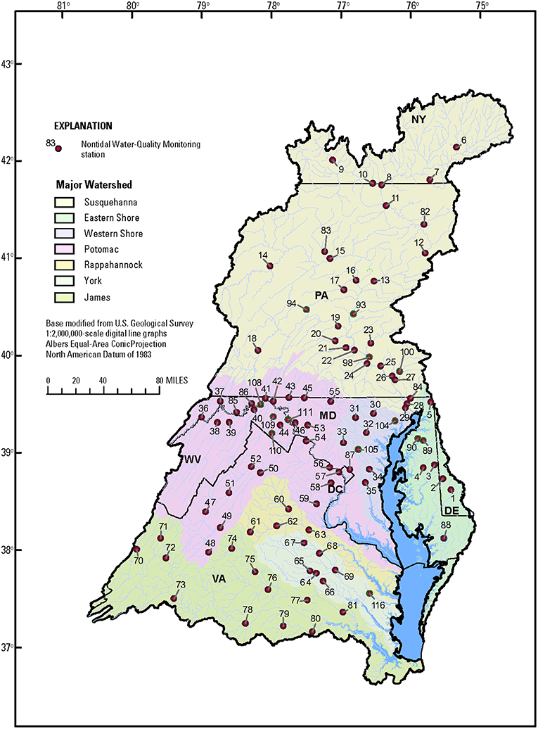
Figure 1. Map of the Chesapeake Bay watershed and sites in the Chesapeake Bay Nontidal Monitoring Network.

TABLE 1

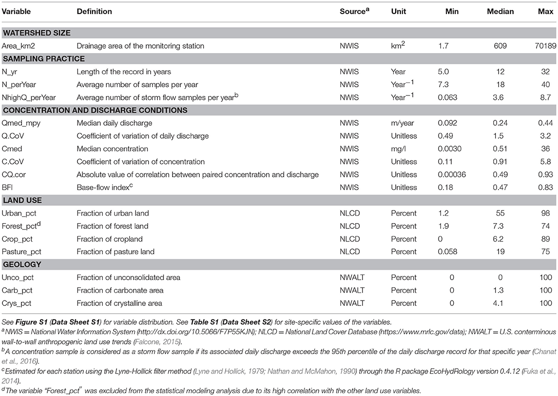
Table 1. List of explanatory variables and their definitions, units, and data sources.

Sites in this network have been sampled using standardized protocols and quality-assurance procedures designed to compute pollutant loads and assess changes in pollutant loads over time. Primary water-quality constituents involved TN, NO_x, TP, PO₄, and SS. Routine samples are collected monthly, and eight additional storm-event samples are collected per year to obtain at least 20 samples per year (Tango and Batiuk, 2016). Samples are collected by nine agencies and are analyzed by five laboratories according to standard operating procedures that conform to Nontidal Monitoring Network protocols and quality-control specifications (U. S. Environmental Protection Agency, 2010; Tango and Batiuk, 2016).

WRTDS Estimation Bias

Water-quality concentration and daily river discharge data have been compiled and analyzed by Moyer et al. (2017) to estimate daily concentrations and fluxes using WRTDS. Functionally, for each day in the observed record, WRTDS develops one separate regression model to estimate constituent concentration. It pre-screens the entire concentration data set and selects samples that are sufficiently “close” to the estimation day in three dimensions, i.e., time, season, and discharge. The selected samples are used to build a weighted regression model and the fitted coefficients are used to estimate concentration on the estimation day by substituting known values of time and daily discharge. To expedite the estimation, the steps above are conducted on a grid network formed by time and log-discharge. For the time axis (x-axis), grid values are spaced 1/16th of a year apart from the beginning year to the end year of the record. For the log-discharge axis (y-axis), 14 grid values are spaced with equal distance for the discharge range from five percent below the minimum discharge to five percent above the maximum discharge in the record—see Hirsch and De Cicco (2015) or Zhang et al. (2016) for examples of the grid. For each grid point, WRTDS develops a separate weighted regression model, which results in an estimated concentration “surface” as functions of time and log-discharge. Daily concentration is then estimated using a bi-linear interpolation of this regression surface, which is then multiplied by daily discharge to compute daily flux. Full estimation details are described in Hirsch and De Cicco (2015). WRTDS is currently (2018) implemented through the Exploration and Graphics for RivEr Trends (EGRET) R package (Hirsch and De Cicco, 2015).

An important point to note is that WRTDS is a highly flexible method, which can be over fitted to the data, particularly to the more extreme values in the data set. Toward that end, WRTDS uses a “leave-one-out-cross-validation” approach to compute the estimated concentrations (Hirsch and De Cicco, 2015). For each observation in the concentration record, WRTDS runs the weighted regression for that specific discharge and time, but with that specific observation left out of the data set. This cross-validation approach provides a more realistic evaluation of the model's ability to make predictions.

In this work, we downloaded the published R workspaces for the Chesapeake Bay Nontidal Water-Quality Monitoring Network for all applicable sites and constituents (Moyer et al., 2017). There are 100, 68, 90, 77, and 90 sites for TN, NO_x, TP, PO₄, and SS, respectively, totaling 425 site-constituent combinations. For each site-constituent combination, we used the fluxBiasStat function in the EGRET R package version 2.6.0 to quantify the bias in estimated daily flux, relative to observed daily flux, on the subset of days having observed concentration data. It is defined as

$\begin{array}{l}\left(meanofestimateddailyflux\text{ - }meanofobserveddailyflux\right)/\hfill \\ meanofobserveddailyflux\text{, or}\hfill \\ \left(meanofestimateddailyflux\text{ / }meanofobserveddailyflux\right)-1\hfill \end{array}$

This metric was selected for model evaluation for two reasons: (1) water resource managers are often interested in average annual and long-term mean fluxes and (2) it is a standard output of WRTDS. We note that there are other metrics that may be used for model evaluation, e.g., the Nash-Sutcliff efficiency, but we focused on the bias statistic in our current work. In experiments with records having dense (in some cases nearly daily) sampling, this statistic was found by Hirsch (2014) to be a useful, although non-linear, predictor of bias in annual flux estimates made using WRTDS on sub-sampled concentration data, relative to more accurate estimates computed directly from the full set of concentration observations; see Hirsch (2014) for details.

We also modified the fluxBiasStat function to quantify the bias in estimated concentration, defined as,

$\begin{array}{l}\begin{array}{l}(meanofestimateddailyconcentration\text{ / }meanofobserved\hfill \\ dailyconcentration)-\mathit{1}\hfill \end{array}\hfill \end{array}$

For the purpose of our work, the terms “flux estimation bias” and “concentration estimation bias” refer to the flux bias statistic and concentration bias statistic, respectively. These metrics provide a comparison between estimated daily load (or daily concentration) and observed daily load (or daily concentration) for the entire period of analysis and, for flux, provide useful indices of the bias in annual flux estimates derived from WRTDS relative to the “true” annual value that would have been computed directly, had daily concentration observations been available. In this work, we have evaluated patterns of both the flux bias and the concentration bias. These bias values are summarized in Table S1 (Data Sheet S2).

Explanatory Variables

To explain the observed patterns in WRTDS estimation bias, a set of explanatory variables (n = 17) were considered (Table 1). These variables fall into the categories of watershed size (n = 1), sampling practice (n = 3), concentration and discharge conditions (n = 6), land use (n = 4), and geology (n = 3). For each monitoring site, land use variables, expressed in the unit of percent, were quantified using the National Land Cover Database (NLCD) (Multi-Resolution Land Characteristics Consortium, 2018). We chose to use the NLCD data for year 2001 because it is roughly in the middle of the WRTDS analysis period (1985–2016). Geology variables, also expressed in percent, were obtained from the U.S. conterminous wall-to-wall anthropogenic land use trends (NWALT) dataset (Falcone, 2015). Similarly, we chose to use data associated with year 2002. Watershed size information was extracted from the published R workspaces (Moyer et al., 2017). BFI, the ratio between baseflow and total riverflow, was calculated using the Lyne-Hollick filter method (Lyne and Hollick, 1979; Nathan and McMahon, 1990) through the R package EcoHydRology version 0.4.12 (Fuka et al., 2014). All the other variables were calculated using the river discharge and concentration records stored in the published R workspaces (Moyer et al., 2017), which were originally retrieved from the U.S. Geological Survey National Water Information System (NWIS; http://dx.doi.org/10.5066/F7P55KJN) and the Chesapeake Bay Program Water Quality Database (https://www.chesapeakebay.net/what/downloads/cbp_water_quality_database_1984_present). In the calculation of NhighQ_perYear, a concentration sample is considered as a storm flow sample if its associated daily discharge exceeds the 95th percentile of the daily discharge record for that specific year (Chanat et al., 2016). The distributions of all explanatory variables are shown in Figure S1 (Data Sheet S1) and their site-specific values are summarized in Table S1 (Data Sheet S2).

The explanatory variables were analyzed in terms of multicollinearity. Specifically, we calculated the Spearman's rank correlation between each two variables as well as the variance inflation factor (VIF). In general, multicollinearity is considered severe if VIF > 10 (Kutner et al., 2004). Our results show that only Forest_pct has a VIF >10, which is strongly correlated with Crop_pct (correlation = 0.67). Thus, Forest_pct was excluded from subsequent statistical analysis.

Statistical Modeling

Three statistical approaches were used to examine the relationship between WRTDS estimation bias and the compiled set of explanatory variables. These approaches are generalized additive model (GAM), classification and regression tree (CART), and random forest (RF) (Hastie et al., 2009). GAM is a relaxed version of linear models by adding the flexibility of additive models. As a semi-parametric model, GAM allows the linear terms in the model to be any desired function of the covariate or covariates rather than strictly linear functions. CART is a non-parametric model that recursively partitions data and uses a very simple model within each partition. Its advantages include quick insight into data patterns and relationships using simple tools such as tree plots. Its basic algorithm involves growing the tree and pruning the tree. RF is an ensemble non-parametric model that builds multiple decision trees and merges the trees together to get a more accurate and stable prediction. RF is a flexible, easy to use machine learning algorithm that is widely used for its simplicity and its ability to handle both classification and regression tasks.

We used the R packages mgcv (version 1.8), rpart (version 4.1), and randomForest (version 4.6) for implementing the GAM, CART, and RF models, respectively. The modeling analysis was done for each individual constituent and for all constituents considered together. Model output was diagnosed, and the relative importance of each explanatory variable was extracted, which represent the relative significance of each variable in determining the estimation bias. For each of the three model types, we scaled the variable importance score of each variable by their sum, so the scaled scores summed to be one. We adopted a multiple-model approach to consider the variable importance scores from all three models. Specifically, we calculated the average of scaled scores from the three model types for each explanatory variable and used these average scores to rank the variables.

Finally, dichotomic tree plots were developed from the CART model output using the fancyRpartPlot function in the rpart R package (version 4.1). These plots show whether estimation bias is large or small while an explanatory variable exceeds an algorithm-determined threshold. Such tree plots can provide complementary information to the variable importance scores, because the latter cannot reveal any information on how the variables influence the bias.

Results

Distribution of WRTDS Estimation Bias

Flux estimation bias is summarized with boxplots in Figure 2A. In general, sediment-associated constituents tend to have larger flux biases than dissolved constituents–the median bias follows the general order of SS > TP > PO₄ > TN ≈ NO_x. Median TN and NO_x bias statistics were near zero, with an equal distribution of small positive and negative bias. TP, PO₄, and SS each showed a median positive bias across sites of <18% for flux (Figure 2A) and <7% for concentration (Figure 3A). The bias for TN flux is almost identical to that of NO_x flux, reflecting the dominance of NO_x in TN flux. These two constituents also show very narrow ranges in bias with medians of ~0.3%. The bias for TP flux is moderately larger than that of PO₄ flux, because TP flux is more dominated by particulate P in many river systems. The two constituents also show wider ranges in bias than TN and NO_x, but their 3rd quantiles are still below 16%. The bias for SS flux has the widest range among all constituents, with a median of ~18%, a third quantile of 47%, and a maximum of 89%.

FIGURE 2

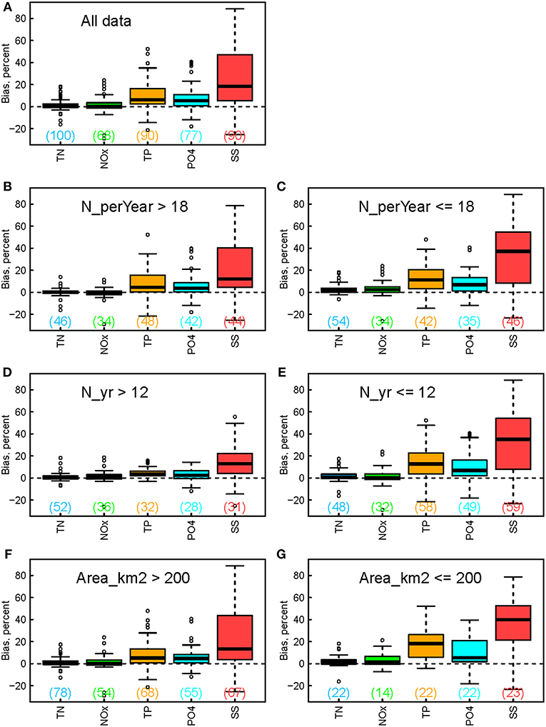
Figure 2. Boxplots showing the estimation bias for constituent flux for (A) all data and (B-G) their subsets. The subsets correspond to different groups of (B,C) sampling frequency, (D,E) sampling record length, and (F,G) watershed size. Numbers in the brackets indicate numbers of applicable sites for each boxplot.

FIGURE 3

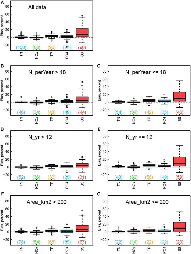
Figure 3. Boxplots showing the estimation bias for constituent concentration for (A) all data and (B-G) their subsets. The subsets correspond to different groups of (B,C) sampling frequency, (D,E) sampling record length, and (F,G) watershed size. Numbers in the brackets indicate numbers of applicable sites for each boxplot.

Flux estimation bias is further broken down to subgroups to provide clues on the effects of sampling frequency (Figures 2B,C), sampling record length (Figures 2D,E), and watershed size (Figures 2F,G). For N_perYear, the median value, i.e., 18 year⁻¹, is used as the cutoff, which is also close to the sampling protocol of 20 year⁻¹. For N_yr, the median value, i.e., 12 years, is used as the cutoff. For Area_km2, the median value is 609 km², but 200 km² is used as the cutoff to capture the patterns at small watersheds. Several important patterns have emerged. First, the general ranking of constituent flux bias—i.e., SS > TP > PO₄ > TN ≈ NO_x—remains valid for these different subgroups of sites. Second, flux bias for TN and NO_x is still centered around zero with narrow ranges. By contrast, the other three constituents, especially SS, show contrasting patterns between different site conditions: flux bias tends to be larger for sites with smaller sampling frequencies (Figure 2C vs. Figure 2B), shorter sampling record lengths (Figure 2E vs. Figure 2D), and smaller watershed sizes (Figure 2G vs. Figure 2F).

Concentration estimation bias is summarized with boxplots in Figure 3, using the same y-axis scale as in Figure 2 to aid comparison with flux bias. First, the general ranking of flux bias remains valid for concentration bias for all data (Figure 3A) and for different subgroups (Figures 3B–G). Second, as was the case with flux bias, concentration bias for TN and NO_x is centered around zero in all plots. Third, the other three constituents, especially SS and TP, show generally smaller concentration bias than their flux bias. The median concentration bias for TP and PO₄ is 3% or smaller, close to the nearly unbiased status of TN and NO_x estimates. SS concentration bias has a median of 7% and 3rd quantile of 22%, about only half of those statistics for SS flux bias. Fourth, SS still shows contrasting patterns between different site conditions: its concentration bias tends to be larger for sites with smaller sampling frequencies (Figure 3C vs. Figure 3B), shorter sampling record lengths (Figure 3E vs. Figure 3D), and smaller watershed sizes (Figure 3G vs. Figure 3F). However, such contrast appears to be no longer applicable to TP and PO₄.

Importance of the Explanatory Variables

In contrast to the boxplots presented above, multivariate approaches (i.e., GAM, CART, and RF) allowed the potential effects of the explanatory variables to be evaluated simultaneously and ranked in terms of their relative importance in determining WRTDS estimation bias (Figure 4 and Table 2). For flux estimation bias (Figure 4A and Table 2), C.CoV is the most influential variable, followed by Q.CoV, N_yr, Cmed, BFI, CQ.cor, Area_km2, and Qmed_mpy. The land use and geology variables appear to be the least influential in determining flux bias. For concentration bias (Figure 4B and Table 2), C.CoV is again the most influential variable. The top-eight variables remain almost the same as in the case of flux bias; the only new top-eight variables for concentration bias are two land use variables (Crop_pct and Pasture_pct), which replace Area_km2 and Qmed_mpy. Consistent with flux bias, concentration bias seems to be least influenced by the geology variables.

FIGURE 4

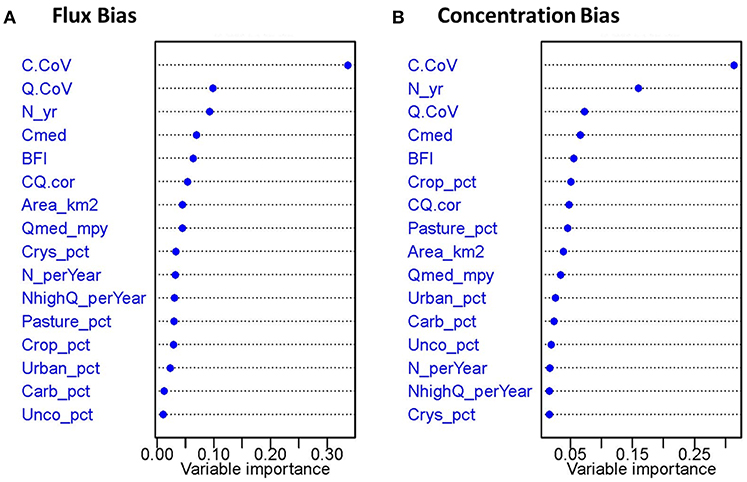
Figure 4. Variable importance ranking from the highest to the lowest based on the three model types developed for constituent (A) flux bias and (B) concentration bias for all site-constituent combinations. See Table 2 for numeric rankings used to calculate variable importance, as described in section Statistical Modeling.

TABLE 2

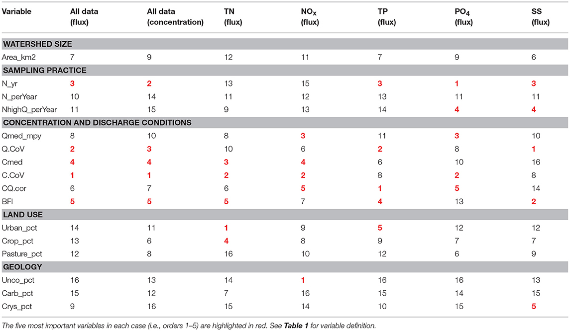
Table 2. Numeric ranking of explanatory variables' importance for flux bias of all constituents, concentration bias of all constituents, and flux bias of each individual constituent.

The relative importance of explanatory variables appears to be constituent-specific. For brevity, we focus only on constituent flux bias and the top-five variables for each constituent (Table 2). For the category of watershed size, none of the five constituents has Area_km2 in the top-five variable list. For the category of sampling practice, N_yr is on the top-five lists of TP, PO₄, and SS, and NhighQ_perYear is on the top-five lists of PO₄ and SS. For the category of concentration and discharge conditions, every variable is on the top-five lists for at least two constituents. In particular, C.CoV has a high ranking for TN, NO_x, and PO₄, while Q.CoV has a high ranking for SS and TP. For the category of land use, Urban_pct is on the top-five lists of TN and TP, and Crop_pct is on the top-five list of TN. Finally, for the category of geology, Unco_pct is on the top-five list of NO_x and Crys_pct is on the top-five list of SS.

Insights From CART Trees

While the relative variable importance ranking can help identify the most influential variables, they cannot provide any information on how the variables influence estimation bias. Thus, we used the CART model output to develop dichotomic tree plots to better visualize the effects of key variables. These plots are presented in Figures 5–7 and Figures S2–S4 (Data Sheet S1) for different constituents. For brevity, we elaborate on NO_x and SS below to represent a dissolved constituent and a particulate constituent, respectively. These tree plots reveal changes in WRTDS estimation bias when an explanatory variable exceeds an algorithm-determined threshold. (Note that these plots were based on CART only, whereas the variable importance scores in section Importance of the Explanatory Variables were based on all three statistical models.)

FIGURE 5

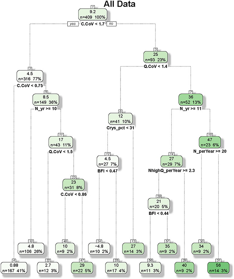
Figure 5. Regression and classification tree developed for constituent flux bias for all site-constituent combinations. In each node, the top number represents the average bias (percent) of cases and the bottom numbers represent the number of cases and the percentage of cases (in bracket). Of the 425 cases for all site-constituent combinations, 16 were excluded due to missing values in land use and/or geology variables.

FIGURE 6

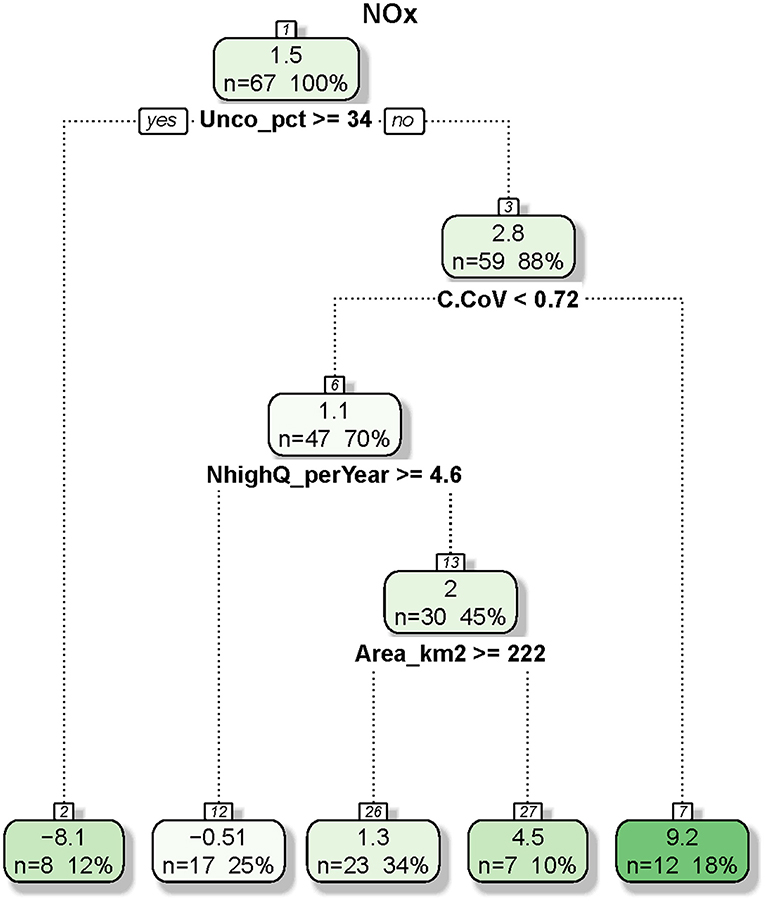
Figure 6. Regression and classification tree developed for constituent flux bias for nitrate-plus-nitrite (NO_x). In each node, the top number represents the average bias (percent) of cases and the bottom numbers represent the number of cases and the percentage of cases (in bracket). Of the 68 cases for NO_x, one was excluded due to missing values in land use and/or geology variables.

FIGURE 7

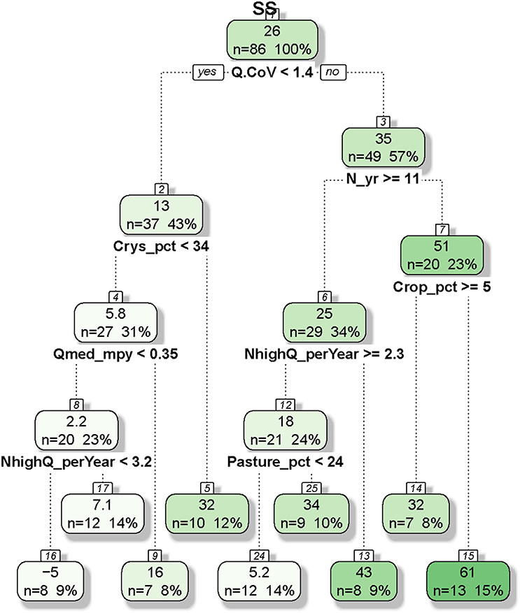
Figure 7. Regression and classification tree developed for constituent flux bias for suspended sediment (SS). In each node, the top number represents the average bias (percent) of cases and the bottom numbers represent the number of cases and the percentage of cases (in bracket). Of the 90 cases for SS, four were excluded due to missing values in land use and/or geology variables.

Figure 5 shows the CART tree plot for flux bias with all constituents and sites considered. The first split is based on C.CoV with a threshold of 1.7. The top node, with a mean bias of 9.2%, is split to child nodes of small bias (mean: 4.5%) for small C.CoV and large bias (mean: 25%) otherwise. In other words, cases with larger concentration variabilities are more difficult to accurately estimate, an inference consistent with the variable importance ranking (Figure 4, Table 2). For small C.CoV cases, the node is further split by C.CoV with a new threshold of 0.75, again with small C.CoV corresponding to small bias (mean: 0.88%) and large C.CoV corresponding to large bias (mean: 8.5%). The latter child node is then split by N_yr with a threshold of 10 years, with large N_yr corresponding to small bias (mean: 4.8%) and small N_yr corresponding to large bias (mean: 17%). Back to the right at the top node of the tree, the child node is further split by Q.CoV with a threshold of 1.4, with small Q.CoV leading to small bias (mean: 12%). The next levels of split are associated several variables, with smaller bias corresponding to smaller Crys_pct, smaller BFI, larger N_yr, larger N_perYear, and larger NhighQ_perYear at the various splits. Overall, the subgroup with the highest bias (mean: 56%) has the characteristics of large C.CoV (>1.7), large Q.CoV (>1.4), small N_yr (<11 years), and small N_perYear (<20 year⁻¹). This result highlights the importance of sampling practice in determining flux bias for cases where C.CoV and Q.CoV are both relatively large.

The CART tree for NO_x flux bias is considerably simpler (Figure 6). At the top node, NO_x flux has a mean bias of 1.5%, which is split by Unco_pct with a threshold of 34%. For sites with Unco_pct >34%, NO_x flux bias becomes strongly negative with a mean of −8.1%. For sites with Unco_pct <34%, NO_x flux bias is slightly positive with a mean of 2.8%. This important role of Unco_pct is consistent with the variable importance ranking result for NO_x (Table 2). The latter child node is further split by C.CoV with a threshold of 0.72, with small C.CoV leading to small bias (mean: 1.1%) and large C.CoV leading to large bias (mean: 9.2%). The node with mean bias of 1.1% is then further split by two variables, with small bias corresponding to large NhighQ_perYear and large Area_km2. Overall, the subgroup with the highest bias (mean: 9.2%) has the characteristics of small Unco_pct (<34%) and large C.CoV (>0.72), although it should be noted that the subgroup with large negative bias (mean: −8.1%) corresponds to large Unco_pct (>34%).

The CART tree for SS flux bias (Figure 7) is quite different from the tree for NO_x. At the top node, SS flux has a mean bias of 26%, which is split by Q.CoV with a threshold of 1.4, leading to child nodes of small bias (mean: 13%) for small Q.CoV and large bias (mean: 35%) otherwise. This important role of Q.CoV is consistent with the variable importance ranking result for SS (Table 2). For the latter child node, it is further split by N_yr with a threshold of 11 years, with large N_yr corresponding to small bias (mean: 25%) and small N_yr corresponding to large bias (mean: 51%). These two child nodes are further split by NhighQ_perYear, Pasture_pct, and Crop_pct, with large NhighQ_perYear, small Pasture_pct, and large Crop_pct corresponding to low biases at the various splits. Back to the left at the top node of the tree, the child node is further split by Crys_pct, Qmed_mpy, and NhighQ_perYear, with small biases associated with small Crys_pct, small Qmed_mpy, and small NhighQ_perYear at the various splits. Two land use variables appear on the SS tree, but they seem to have opposite effects: large Pasture_pct leads to large bias, while large Crop_pct leads to small bias. Overall, the subgroup with the highest bias (mean: 61%) has the characteristics of large Q.CoV (>1.4), small N_yr (<11 years), and small Crop_pct (<5%).

Discussion

Accurate quantification of constituent flux has major implications to ecological conditions of downstream receiving waters (e.g., lakes, estuaries), particularly from a mass-balance perspective. Our analysis of WRTDS estimation bias (Figure 2) showed that sediment-associated constituents (SS and TP) tend to have larger flux biases than dissolved constituents (TN and NO_x), as observed in several previous investigations (Moyer et al., 2012; Chanat et al., 2016; Zhang and Ball, 2017). The breakdown of estimation bias into different subgroups highlighted the effects of sampling practice and watershed size: flux bias for particulate constituents, especially SS, tends to be larger for sites with smaller sampling frequencies, shorter sampling record lengths, and smaller watershed sizes.

In addition, accurate quantification of constituent concentration is critical to understanding in-stream processes such as biogeochemical cycling. This work provided new information on concentration estimation bias (Figure 3), which has not been commonly reported in the literature. We found that concentration bias follows the general ranking of flux bias in terms of median—i.e., SS > TP > PO₄ > TN ≈ NO_x. In addition, constituents with nearly unbiased flux estimates, i.e., TN and NO_x, have nearly unbiased concentration estimates for most sites. Constituents with positively biased flux estimates, i.e., TP, PO₄, and SS, tend to have less biased concentration estimates than corresponding flux estimates. These results should lend more confidence to research that uses WRTDS to generate concentration estimates. Lastly, we found that only SS has strongly contrasting patterns in concentration bias between different conditions of sampling practice and watershed size.

Characteristics of individual monitoring sites have strong effects on WRTDS flux estimation bias. While prior studies have typically used a sub-sampling methodology from relatively high-frequency data to quantify the effects of factors such as watershed size, sampling strategy, and length of record (Johnes, 2007; Birgand et al., 2010, 2011; Defew et al., 2013; Kumar et al., 2013; Horowitz et al., 2014; Elwan et al., 2018), our analysis was aimed toward a simultaneous evaluation of the candidate variables. When all constituents are considered, both flux bias and concentration bias are most affected by the same top-five variables, namely, C.CoV, Q.CoV, N_yr, Cmed, and BFI (Figure 4 and Table 2), stressing the importance of concentration and discharge variability, the length of concentration record, and the relative contribution of baseflow vs. rapid flow in determining bias. None of the watershed size, land use, or geology variables appears on these two lists. When each constituent is analyzed separately, flux estimation bias appears to be affected by different combinations of variable categories (Table 2), but almost all candidate variables appear on the top-five list for at least one constituent. For the top variables listed above, C.CoV has high rankings for TN, NO_x, and PO₄, while Q.CoV has high rankings for SS and TP. Such contrast shows that the flux bias of particulate constituents is more affected by flow variability, whereas the flux bias of dissolved constituents is more affected by concentration variability, reflecting the distinction of transport mechanisms between particulate and dissolved constituents. In addition, N_yr has high rankings for TP, PO₄, and SS, suggesting the importance of the length of concentration record for these constituents.

The CART tree plots provided additional insights on how the variables influence flux bias. For all constituents considered (Figure 5), the subgroup with the highest bias (mean: 56%) has the characteristics of large C.CoV (>1.7), large Q.CoV (>1.4), small N_yr (<11 years), and small N_perYear (<20 year⁻¹). The implication is that resource managers should expect large flux biases for river and streams that have large concentration and discharge variabilities, small lengths of concentration record, and small sampling frequencies. Thus, river monitoring may target the sites where C.CoV and Q.CoV are relatively large–for these sites, it can be particularly useful to increase the length of concentration record and/or the sampling frequency in order to reduce the flux bias.

The CART tree plots also demonstrated that flux estimation bias of each constituent is determined by a unique set of candidate variables (Figures 6, 7 and Figures S2–S4). For NO_x flux (Figure 6), the subgroup with the highest bias (mean: 9.2%) has the characteristics of small Unco_pct (<34%) and large C.CoV (>0.72). For SS flux (Figure 7), the subgroup with the highest bias (mean: 61%) has the characteristics of large Q.CoV (>1.4), small N_yr (<11 years), and small Crop_pct (<5%). These results suggest that resource managers should set different expectations on different constituents—i.e., large NO_x biases for rivers and streams with large concentration variabilities and small presence of unconsolidated area and large SS biases for rivers and streams with large discharge variabilities, small lengths of concentration record, and small presence of cropland. For SS, monitoring priority should be given to sites with large Q.CoV and small Crop_pct, where bias is expected to decrease by increasing N_yr. For NO_x, sites with large Unco_pct (>34%) are generally located in the Coastal Plain areas on the Eastern Shore and Western Shore (e.g., Choptank River, Mattaponi River, and Nanticoke River—see Figure 1). These watersheds are underlain by unconsolidated sediments (e.g., clay, sand) and groundwater flows through spaces between the sediment grains (Fenneman and Johnson, 1946). The subsurface transport of NO_x may complicate its concentration signals manifested in the rivers, resulting in the relatively high biases at these low-lying coastal locations.

Overall, these findings may be useful for identifying sites with large biases, modifying monitoring practice at existing sites to reduce those biases, and choosing new monitoring locations in the Chesapeake Bay watershed and beyond. WRTDS is shown to be appropriate for the majority of sites in this network. Compared with the previously used LOADEST method, WRTDS has generally enhanced our method capability to estimate riverine concentrations and fluxes (Moyer et al., 2012; Chanat et al., 2016). However, WRTDS estimation for small watersheds (such as headwater watersheds) may not be as satisfactory as for large watersheds, particularly for sediment and phosphorus (Figures 2F,G). For such watersheds, sampling design that was aimed toward understanding the subtlety of nitrogen processes needs to be improved with modified sampling practice to better capture the dynamics of sediment and phosphorus. In this regard, high-frequency (e.g., 15-min to hourly) water-quality samples can be particularly useful, which can be collected directly (e.g., nitrate sensors) or derived through surrogates (e.g., turbidity, pH, specific conductance) (Pellerin et al., 2016). It has been established that the surrogate approach can generate flux estimates that have reduced uncertainty (Jastram et al., 2009; Pellerin et al., 2014; Stutter et al., 2017). WRTDS, as many other statistical approaches, is subject to the limitation of data availability. For SS and TP, more concentration samples need to be collected to better represent storm flow conditions (Sprague, 2001; Ide et al., 2012; Chanat et al., 2016; Zhang and Ball, 2017). Currently, the Chesapeake network engages a sampling protocol that collects at least 20 samples per year, with eight samples targeted toward storm flow conditions (Chanat et al., 2016). To further reduce estimation bias, more investment may be needed to increase the number of water-quality observations collected each year during storm flow periods. Given that funding resources may not be available to enhance storm flow sampling and/or high-resolution sampling at all locations in the network, monitoring can be strategically refined by allocating funding resources to monitoring locations where estimation bias is most affected by the availability (i.e., length and frequency) of water-quality samples. For example, when all constituents are considered, the subgroup with the highest bias has the characteristics of large C.CoV (>1.7), large Q.CoV (>1.4), small N_yr (<11 years), and small N_perYear (<20 year⁻¹). Thus, it may be most fruitful to increase N_yr and/or N_perYear at sites that have large C.CoV, large Q.CoV, and small N_yr. More broadly, for many monitoring sites in the United States and beyond, where only river discharge data are available, the variable Q.CoV may serve as a preliminary guideline—i.e., if new water-quality monitoring was to established, priority should be given to locations where Q.CoV is small.

In future work, we recommend including sites from other geographical regions to place these results into a more generalizable context to inform river monitoring and management. This is feasible, since WRTDS has been adopted in surface water-quality studies in many regions. In addition, the modeling approaches adopted in this work can be adapted to other water-quality constituents, such as chloride, pesticides, and organic carbon. Furthermore, this work is limited to flux and concentration estimates and it remains unclear how the bias of these estimates interacts with the accuracy of temporal trends, which is another important aspect of surface water-quality research. Lastly, this work focused entirely on traditional, discretely sampled data. In this regard, future research may explore how estimation bias might be affected by the addition of high-frequency data.

Conclusions

We synthesized and compared WRTDS estimation bias for five common water-quality constituents for a range of rivers and streams in the Chesapeake Bay watershed (including headwater sites) and investigated the relative importance of various explanatory variables in determining the magnitude of estimation bias. For both concentration and flux, estimation bias follows the general order of SS > TP > PO₄ > TN ≈ NO_x. Median TN and NO_x bias statistics were near zero, with an equal distribution of small positive and negative bias. TP, PO₄, and SS each showed a median positive bias across sites of <18% for flux and <7% for concentration. Particulate constituents, especially SS, tend to have larger bias at sites with lower sampling frequencies, shorter water-quality record lengths, and smaller watershed sizes. Three multivariate models were used to investigate the relative importance of various factors in determining estimation bias. Results showed that both flux and concentration biases are most affected by concentration and discharge variabilities as well as the length of the water-quality record. In comparison, flux bias of particulate constituents is more affected by flow variability, whereas flux bias of dissolved constituents is more affected by concentration variability. Moreover, analysis using classification and regression trees provided additional information on how the factors affected flux bias: when all site-constituent combinations are considered, large flux biases are more likely associated with sites with large concentration and discharge variabilities, small lengths of concentration record, and small sampling frequencies. Overall, these findings may be useful for identifying sites with large biases, modifying monitoring practice at existing sites to reduce those biases, and choosing new monitoring locations in the Chesapeake Bay watershed and beyond. Given that funding resources may not be available to maintain or enhance the sampling at all locations in this monitoring network (or others), monitoring can be strategically refined by allocating resources to locations where estimation bias is most affected by the availability (i.e., length and frequency) of water-quality samples.

Data Availability

River monitoring data used in this research are available online through the U.S. Geological Survey National Water Information System (https://nwis.waterdata.usgs.gov/nwis) and Chesapeake Bay Program Water Quality Database (https://www.chesapeakebay.net/what/downloads/cbp_water_quality_database_1984_present). The published R workspaces for the Chesapeake Bay Nontidal Network stations are available online through the U.S Geological Survey ScienceBase (https://doi.org/10.5066/F7RR1X68).

Author Contributions

QZ conducted the statistical analyses, developed the models, produced the tables and figures for the manuscript, and led the writing of the manuscript. All authors contributed to the interpretation of results and the writing of the manuscript.

Funding

This work was supported by the U.S. Environmental Protection Agency under grant EPA/CBP Technical Support 2017 (No. 07-5-230480).

Conflict of Interest Statement

The authors declare that the research was conducted in the absence of any commercial or financial relationships that could be construed as a potential conflict of interest.

Acknowledgments

We would like to thank Andy Sekellick (USGS) for providing the data on land use and geology variables. Casey Lee (USGS) and two journal reviewers are acknowledged for their comments on an earlier version of this manuscript. Any use of trade, firm, or product names is for descriptive purposes only and does not imply endorsement by the U.S. Government. This is contribution no. 5540 of the University of Maryland Center for Environmental Science.

Supplementary Material

The Supplementary Material for this article can be found online at: https://www.frontiersin.org/articles/10.3389/fevo.2019.00109/full#supplementary-material

References

Birgand, F., Faucheux, C., Gruau, G., Augeard, B., Moatar, F., and Bordenave, P. (2010). Uncertainties in assessing annual nitrate loads and concentration indicators: part 1. Impact of sampling frequency and load estimation algorithms. Transact. ASABE 53, 437–446. doi: 10.13031/2013.29584

CrossRef Full Text | Google Scholar

Birgand, F., Faucheux, C., Gruau, G., Moatar, F., and Meybeck, M. (2011). Uncertainties in assessing annual nitrate loads and concentration indicators: part 2. deriving sampling frequency charts in Brittany, France. Transact. ASABE 54, 93–104. doi: 10.13031/2013.36263

CrossRef Full Text | Google Scholar

Bowes, M. J., Smith, J. T., Jarvie, H. P., and Neal, C. (2008). Modelling of phosphorus inputs to rivers from diffuse and point sources. Science of the Total Environment 395, 125–138. doi: 10.1016/j.scitotenv.2008.01.054

PubMed Abstract | CrossRef Full Text | Google Scholar

Chanat, J. G., Moyer, D. L., Blomquist, J. D., Hyer, K. E., and Langland, M. J. (2016). Application of a Weighted Regression Model for Reporting Nutrient and Sediment Concentrations, Fluxes, and Trends in Concentration and Flux for the Chesapeake Bay Nontidal Water-Quality Monitoring Network, Results Through Water Year 2012. U.S. Geological Survey Scientific Investigations Report 2015–5133. doi: 10.3133/sir20155133

CrossRef Full Text

Cohn, T. A. (2005). Estimating contaminant loads in rivers: an application of adjusted maximum likelihood to type 1 censored data. Water Resour. Res. 41, 1–13. doi: 10.1029/2004wr003833

CrossRef Full Text | Google Scholar

Cohn, T. A., Caulder, D. L., Gilroy, E. J., Zynjuk, L. D., and Summers, R. M. (1992). The validity of a simple statistical model for estimating fluvial constituent loads: an empirical study involving nutrient loads entering Chesapeake Bay. Water Resour. Res. 28, 2353–2353. doi: 10.1029/92wr01008

CrossRef Full Text | Google Scholar

Cohn, T. A., Delong, L. L., Gilroy, E. J., Hirsch, R. M., and Wells, D. K. (1989). Estimating constituent loads. Water Resour. Res. 25, 937–942. doi: 10.1029/WR025i005p00937

CrossRef Full Text | Google Scholar

Corsi, S. R., De Cicco, L. A., Lutz, M. A., and Hirsch, R. M. (2015). River chloride trends in snow-affected urban watersheds: increasing concentrations outpace urban growth rate and are common among all seasons. Sci. Total Environ. 508, 488–497. doi: 10.1016/j.scitotenv.2014.12.012

PubMed Abstract | CrossRef Full Text | Google Scholar

Crowder, D. W., Demissie, M., and Markus, M. (2007). The accuracy of sediment loads when log-transformation produces nonlinear sediment load–discharge relationships. J. Hydrol. 336, 250–268. doi: 10.1016/j.jhydrol.2006.12.024

CrossRef Full Text | Google Scholar

Defew, L. H., May, L., and Heal, K. V. (2013). Uncertainties in estimated phosphorus loads as a function of different sampling frequencies and common calculation methods. Mar. Freshwater Res. 64, 373–386. doi: 10.1071/MF12097

CrossRef Full Text | Google Scholar

Dolan, D. M., Yui, A. K., and Geist, R. D. (1981). Evaluation of river load estimation methods for total phosphorus. J. Great Lakes Res. 7, 207–214. doi: 10.1016/s0380-1330(81)72047-1

CrossRef Full Text | Google Scholar

Elwan, A., Singh, R., Patterson, M., Roygard, J., Horne, D., Clothier, B., et al. (2018). Influence of sampling frequency and load calculation methods on quantification of annual river nutrient and suspended solids loads. Environ. Monit. Assess. 190:78. doi: 10.1007/s10661-017-6444-y

PubMed Abstract | CrossRef Full Text | Google Scholar

Falcone, J. A. (2015). U.S. Conterminous Wall-to-Wall Anthropogenic Land Use Trends (NWALT), 1974–2012. U.S. Geological Survey Data Series 948. Reston, VA. Available online at: https://doi.org/10.3133/ds948

Fenneman, N. M., and Johnson, D. W. (1946). Physiographic Divisions of the Conterminous U. S. U.S. Geological Survey. Reston, VA. Available online at: http://water.usgs.gov/GIS/metadata/usgswrd/XML/physio.xml

Fuka, D., Walter, M., Archibald, J., Steenhuis, T., and Easton, Z. (2014). EcoHydRology: A Community Modeling Foundation for Eco-Hydrology. R Package Version 0.4.12. Available online at: http://CRAN.R-project.org/package=EcoHydRology

Green, C. T., Bekins, B. A., Kalkhoff, S. J., Hirsch, R. M., Liao, L., and Barnes, K. K. (2014). Decadal surface water quality trends under variable climate, land use, and hydrogeochemical setting in Iowa, USA. Water Resour. Res. 50, 2425–2443. doi: 10.1002/2013wr014829

CrossRef Full Text | Google Scholar

Hastie, T., Tibshirani, R., and Friedman, J. (2009). The Elements of Statistical Learning: Data Mining, Inference, and Prediction. New York, NY: Springer-Verlag.

Google Scholar

Hirsch, R. M. (2014). Large biases in regression-based constituent flux estimates: causes and diagnostic tools. J. Am. Water Res. Assoc. 50, 1401–1424. doi: 10.1111/jawr.12195

CrossRef Full Text | Google Scholar

Hirsch, R. M., and De Cicco, L. (2015). User Guide to Exploration and Graphics for RivEr Trends (EGRET) and Dataretrieval: R Packages for Hydrologic Data (Version 2.0, February 2015). U.S. Geological Survey Techniques and Methods Book 4, Chapter A10. Reston, VA

Hirsch, R. M., Moyer, D. L., and Archfield, S. A. (2010). Weighted Regressions on Time, Discharge, and Season (WRTDS), with an application to Chesapeake Bay River inputs. J. Am. Water Res. Assoc. 46, 857–880. doi: 10.1111/j.1752-1688.2010.00482.x

PubMed Abstract | CrossRef Full Text | Google Scholar

Horowitz, A. J., Clarke, R. T., and Merten, G. H. (2014). The effects of sample scheduling and sample numbers on estimates of the annual fluxes of suspended sediment in fluvial systems. Hydrol. Process. 29, 2267–2274. doi: 10.1002/hyp.10172

CrossRef Full Text | Google Scholar

Ide, J., Chiwa, M., Higashi, N., Maruno, R., Mori, Y., and Otsuki, K. (2012). Determining storm sampling requirements for improving precision of annual load estimates of nutrients from a small forested watershed. Environ. Monit. Assess. 184, 4747–4762. doi: 10.1007/s10661-011-2299-9

PubMed Abstract | CrossRef Full Text | Google Scholar

Jastram, J. D., Moyer, D. L., and Hyer, K. E. (2009). A Comparison of Turbidity-Based and Streamflow-Based Estimates of Suspended-Sediment Concentrations in Three Chesapeake Bay Tributaries. U.S. Geological Survey Scientific Investigations Report 2009-5165. Richmond, VA.

Johnes, P. J. (2007). Uncertainties in annual riverine phosphorus load estimation: impact of load estimation methodology, sampling frequency, baseflow index and catchment population density. J. Hydrol. 332, 241–258. doi: 10.1016/j.jhydrol.2006.07.006

CrossRef Full Text | Google Scholar

Kronvang, B., and Bruhn, A. J. (1996). Choice of sampling strategy and estimation method for calculating nitrogen and phosphorus transport in small lowland streams. Hydrol. Process. 10, 1483–1501. doi: 10.1002/(SICI)1099-1085(199611)10:11<1483::AID-HYP386>3.0.CO;2-Y

CrossRef Full Text | Google Scholar

Kumar, S., Godrej, A. N., and Grizzard, T. J. (2013). Watershed size effects on applicability of regression-based methods for fluvial loads estimation. Water Resour. Res. 49, 7698–7710. doi: 10.1002/2013WR013704

CrossRef Full Text | Google Scholar

Kutner, M., Nachtsheim, C., and Neter, J. (2004). Applied Linear Statistical Models. McGraw-Hill Education.

Lee, C. J., Hirsch, R. M., Schwarz, G. E., Holtschlag, D. J., Preston, S. D., Crawford, C. G., et al. (2016). An evaluation of methods for estimating decadal stream loads. J. Hydrol. 542, 185–203. doi: 10.1016/j.jhydrol.2016.08.059

CrossRef Full Text | Google Scholar

Linker, L. C., Batiuk, R. A., Shenk, G. W., and Cerco, C. F. (2013). Development of the Chesapeake Bay watershed total maximum daily load allocation. J. Am. Water Res. Assoc. 49, 986–1006. doi: 10.1111/jawr.12105

CrossRef Full Text | Google Scholar

Littlewood, I. G., and Marsh, T. J. (2005). Annual freshwater river mass loads from Great Britain, 1975–1994: estimation algorithm, database and monitoring network issues. J. Hydrol. 304, 221–237. doi: 10.1016/j.jhydrol.2004.07.031

CrossRef Full Text | Google Scholar

Lyne, V. D., and Hollick, M. (1979). “Stochastic time-variable rainfall-runoff modeling,” in Hydrology and Water Resources Symposium. Perth, WA: Institution of Engineers Australia.

Google Scholar

Moatar, F., Meybeck, M., Raymond, S., Birgand, F., and Curie, F. (2013). River flux uncertainties predicted by hydrological variability and riverine material behaviour. Hydrol. Process. 27, 3535–3546. doi: 10.1002/hyp.9464

CrossRef Full Text | Google Scholar

Moyer, D. L., Hirsch, R. M., and Hyer, K. E. (2012). Comparison of Two Regression-Based Approaches for Determining Nutrient and Sediment Fluxes and Trends in the Chesapeake Bay Watershed. U.S. Geological Survey Scientific Investigations Report 2012–5244. Reston, VA. Available online at: http://pubs.usgs.gov/sir/2012/5244/

Moyer, D. L., Langland, M. J., Blomquist, J. D., and Yang, G. (2017). Nitrogen, Phosphorus, and Suspended-Sediment Loads and Trends Measured at the Chesapeake Bay Nontidal Network Stations: Water Years 1985–2016. U.S. Geological Survey. doi: 10.5066/F7RR1X68.

CrossRef Full Text

Multi-Resolution Land Characteristics Consortium (2018). National Land Cover Database (NLCD). Available online at: https://www.mrlc.gov/finddata.php

Nathan, R. J., and McMahon, T. A. (1990). Evaluation of automated techniques for base flow and recession analyses. Water Resour. Res. 26, 1465–1473. doi: 10.1029/WR026i007p01465

CrossRef Full Text | Google Scholar

Park, Y. S., and Engel, B. A. (2015). Analysis for regression model behavior by sampling strategy for annual pollutant load estimation. J. Environ. Q. 44, 1843–1851. doi: 10.2134/jeq2015.03.0137

PubMed Abstract | CrossRef Full Text | Google Scholar

Pellerin, B. A., Bergamaschi, B. A., Gilliom, R. J., Crawford, C. G., Saraceno, J., Frederick, C. P., et al. (2014). High frequency measurement of nitrate concentration in the Lower Mississippi River, USA. Environ. Sci. Technol. 48, 12612–12619. doi: 10.1021/es504029c

CrossRef Full Text | Google Scholar

Pellerin, B. A., Stauffer, B. A., Young, D. A., Sullivan, D. J., Bricker, S. B., Walbridge, M. R., et al. (2016). Emerging tools for continuous nutrient monitoring networks: sensors advancing science and water resources protection. J. Am. Water Res. Assoc. 52, 993–1008. doi: 10.1111/1752-1688.12386

CrossRef Full Text | Google Scholar

Purina, I., Labucis, A., Barda, I., Jurgensone, I., and Aigars, J. (2018). Primary productivity in the Gulf of Riga (Baltic Sea) in relation to phytoplankton species and nutrient variability. Oceanologia 60, 544–552. doi: 10.1016/j.oceano.2018.04.005

CrossRef Full Text | Google Scholar

Rankinen, K., Keinänen, H., and Cano Bernal, J. E. (2016). Influence of climate and land use changes on nutrient fluxes from Finnish rivers to the Baltic Sea. Agric. Ecosyst. Environ. 216, 100–115. doi: 10.1016/j.agee.2015.09.010

CrossRef Full Text | Google Scholar

Raymond, S., Moatar, F., Meybeck, M., and Bustillo, V. (2013). Choosing methods for estimating dissolved and particulate riverine fluxes from monthly sampling. Hydrol. Sci. J. 58, 1326–1339. doi: 10.1080/02626667.2013.814915

CrossRef Full Text | Google Scholar

Robertson, D. M., and Roerish, E. D. (1999). Influence of various water quality sampling strategies on load estimates for small streams. Water Resour. Res. 35, 3747–3759. doi: 10.1029/1999wr900277

CrossRef Full Text | Google Scholar

Shenk, G. W., and Linker, L. C. (2013). Development and application of the 2010 Chesapeake Bay watershed total maximum daily load model. J. Am. Water Res. Assoc. 49, 1042–1056. doi: 10.1111/jawr.12109

CrossRef Full Text | Google Scholar

Sprague, L. A. (2001). Effects of Storm-Sampling Frequency on Estimation of Water-Quality Loads and Trends in Two Tributaries to Chesapeake Bay in Virginia. US Geological Survey Water-Resources Investigations Report 01-4136. Richmond, VA.

Google Scholar

Sprague, L. A., Hirsch, R. M., and Aulenbach, B. T. (2011). Nitrate in the Mississippi River and its tributaries, 1980 to 2008: are we making progress? Environ. Sci. Technol. 45, 7209–7216. doi: 10.1021/es201221s

PubMed Abstract | CrossRef Full Text | Google Scholar

Stackpoole, S. M., Stets, E. G., Clow, D. W., Burns, D. A., Aiken, G. R., Aulenbach, B. T., et al. (2017). Spatial and temporal patterns of dissolved organic matter quantity and quality in the Mississippi River Basin, 1997–2013. Hydrol. Process. 31, 902–915. doi: 10.1002/hyp.11072

CrossRef Full Text | Google Scholar

Stenback, G. A., Crumpton, W. G., Schilling, K. E., and Helmers, M. J. (2011). Rating curve estimation of nutrient loads in Iowa rivers. J. Hydrol. 396, 158–169. doi: 10.1016/j.jhydrol.2010.11.006

CrossRef Full Text | Google Scholar

Stets, E. G., Lee, C. J., Lytle, D. A., and Schock, M. R. (2018). Increasing chloride in rivers of the conterminous U.S. and linkages to potential corrosivity and lead action level exceedances in drinking water. Sci. Total Environ. 613–614, 1498–1509. doi: 10.1016/j.scitotenv.2017.07.119

CrossRef Full Text | Google Scholar

Stow, C. A., and Borsuk, M. E. (2003). Assessing TMDL effectiveness using flow-adjusted concentrations: a case study of the Neuse River, North Carolina. Environ. Sci. Technol. 37, 2043–2050. doi: 10.1021/es020802p

PubMed Abstract | CrossRef Full Text | Google Scholar

Stutter, M., Dawson, J. J. C., Glendell, M., Napier, F., Potts, J. M., Sample, J., et al. (2017). Evaluating the use of in-situ turbidity measurements to quantify fluvial sediment and phosphorus concentrations and fluxes in agricultural streams. Sci. Total Environ. 607–608, 391–402. doi: 10.1016/j.scitotenv.2017.07.013

CrossRef Full Text | Google Scholar

Tango, P. J., and Batiuk, R. A. (2016). Chesapeake Bay recovery and factors affecting trends: long-term monitoring, indicators, and insights. Reg. Stud. Mar. Sci. 4, 12–20. doi: 10.1016/j.rsma.2015.11.010

CrossRef Full Text | Google Scholar

U. S. Environmental Protection Agency (2010). Chesapeake Bay total Maximum Daily Load for Nitrogen, Phosphorus and Sediment. U.S. Environmental Protection Agency. (Annapolis, MD). Available online at: https://www.epa.gov/chesapeake-bay-tmdl/chesapeake-bay-tmdl-document

Van Meter, K. J., and Basu, N. B. (2017). Time lags in watershed-scale nutrient transport: an exploration of dominant controls. Environ. Res. Lett. 12:8. doi: 10.1088/1748-9326/aa7bf4

CrossRef Full Text | Google Scholar

Vrzel, J., and Ogrinc, N. (2015). Nutrient variations in the Sava River Basin. J. Soils Sediments 15, 2380–2386. doi: 10.1007/s11368-015-1190-7

CrossRef Full Text | Google Scholar

Williams, M. R., King, K. W., Macrae, M. L., Ford, W., Van Esbroeck, C., Brunke, R. I., et al. (2015). Uncertainty in nutrient loads from tile-drained landscapes: effect of sampling frequency, calculation algorithm, and compositing strategy. J. Hydrol. 530, 306–316. doi: 10.1016/j.jhydrol.2015.09.060

CrossRef Full Text | Google Scholar

Worrall, F., Howden, N.J.K., and Burt, T.P. (2013). Assessment of sample frequency bias and precision in fluvial flux calculations - An improved low bias estimation method. J Hydrol. 503, 101–110. doi: 10.1016/j.jhydrol.2013.08.048

CrossRef Full Text | Google Scholar

Zhang, Q., and Ball, W. P. (2017). Improving riverine constituent concentration and flux estimation by accounting for antecedent discharge conditions. J. Hydrol. 547, 387–402. doi: 10.1016/j.jhydrol.2016.12.052

CrossRef Full Text | Google Scholar

Zhang, Q., and Blomquist, J. D. (2018). Watershed export of fine sediment, organic carbon, and chlorophyll-a to Chesapeake Bay: spatial and temporal patterns in 1984–2016. Sci. Total Environ. 619–620, 1066–1078. doi: 10.1016/j.scitotenv.2017.10.279

CrossRef Full Text | Google Scholar

Zhang, Q., Brady, D. C., and Ball, W. P. (2013). Long-term seasonal trends of nitrogen, phosphorus, and suspended sediment load from the non-tidal Susquehanna River Basin to Chesapeake Bay. Sci. Total Environ. 452–453, 208–221. doi: 10.1016/j.scitotenv.2013.02.012

CrossRef Full Text | Google Scholar

Zhang, Q., Brady, D. C., Boynton, W. R., and Ball, W. P. (2015). Long-term trends of nutrients and sediment from the nontidal Chesapeake watershed: an assessment of progress by river and season. J. Am. Water Res. Assoc. 51, 1534–1555. doi: 10.1111/1752-1688.12327

CrossRef Full Text | Google Scholar

Zhang, Q., Harman, C. J., and Ball, W. P. (2016). An improved method for interpretation of riverine concentration-discharge relationships indicates long-term shifts in reservoir sediment trapping. Geophys. Res. Lett. 43, 10,215–210,224. doi: 10.1002/2016gl069945

CrossRef Full Text | Google Scholar