New indicators of ecological resilience and invasion resistance to support prioritization and management in the sagebrush biome, United States

Introduction

Ecosystem transformations to altered or novel ecological states are accelerating across the globe as a result of human perturbations (Díaz et al., 2019) and the introductions and invasions of exotic species that often co-occur with these perturbations (Richardson and Gaertner, 2013; Early et al., 2016). Ongoing climate change is a pervasive, added stressor, which is not only altering ecosystem processes and disturbance regimes, but changing the areas of climatic suitability for invasive species (Nolan et al., 2018). Prioritization of ecological restoration and other management activities where they are likely to have the greatest benefits is essential for addressing this rapid change (Tolvanen and Aronson, 2016). Science-based prioritization of restoration and other management activities in national and regional planning can contribute to creation of sustainable landscapes that maintain both biodiversity and ecosystem services (Brondizio et al., 2019).

Recently, ecological resilience concepts have been operationalized to aid understanding of the environmental factors and ecosystem attributes that determine the recovery potentials of ecosystems and that are needed for effective prioritization (Hirota et al., 2011; Levine et al., 2016; Chambers et al., 2019a; Yao et al., 2021). Ecological resilience (resilience) is the capacity of ecosystems to reorganize and regain their fundamental structure, processes and functioning (i.e., recover) when altered by stresses, like longer and more severe drought, and by disturbances, such as altered fire regimes (Holling, 1973; Scheffer, 2009). Developing an understanding of resistance to invasive species is increasingly important because of the transformative properties of invaders (Richardson and Gaertner, 2013). Resistance to invasion (resistance) is a function of the abiotic and biotic attributes and ecological processes of an ecosystem that limit the population growth of an invading species (D'Antonio and Thomsen, 2004). Resistance to invasion differs among exotic species because it depends on (1) soil and climate suitability for establishment and persistence the invader, and (2) interactions of the invader with the plant community (Chambers et al., 2014a; Brooks et al., 2016).

At the landscape scales relevant to management, the resilience and resistance of ecosystems vary across environmental gradients and can be quantified using measures of environmental factors, including climate, topography, soils, and potential biota (Hirota et al., 2011; Chambers et al., 2019a; Yao et al., 2021). In dryland regions of the United States, these environmental factors form the basis of a landscape-scale classification of ecological site types by the USDA Natural Resources Conservation Service, i.e., the Ecological Site Descriptions (USDA Natural Resources Conservation Service [USDA NRCS], 2022a). Disturbances and stresses that change the structure and composition of plant communities, such as inappropriate livestock grazing, and alter disturbance regimes, such as nonnative plant invasions, can affect the recovery and likelihood of invasion of an ecological site. If these disturbances and stresses are severe enough, they may result in transitions to alternative states as illustrated by state-and-transition models (USDA Natural Resources Conservation Service [USDA NRCS], 2022a). Indicators of resilience and resistance provide information on the likelihood of transitions to alternative states and effectiveness of management actions (Briske et al., 2008; Crist et al., 2019; Chambers et al., 2019a).

Climate and soil water availability are highly effective indicators of resilience and resistance and the likelihood of change in dryland ecosystems (Bestelmeyer et al., 2015). Vegetation dynamics in drylands, including the environmental suitability for an invasive species and the likelihood of transitions to alternative states, are determined largely by climate and soil water availability (Stephenson, 1990; Shriver et al., 2018; O’Connor et al., 2020). These areas have high sensitivity to the landscape variations in climate that influence soil water availability, including patterns of both temperature and precipitation (Renne et al., 2019), and are prone to degradation and vulnerable to climate change (Burrell et al., 2020).

Environmental indicators based on process-based ecohydrological models provide the basis for evaluating both the current effects of environmental conditions and the long-term impact of climate change on dryland resilience and resistance. Quantifying ecologically relevant changes in water availability is difficult in drylands because the response of vegetation to moisture and temperature conditions is not easily explained by meteorological indices or even simple water balance models (McColl et al., 2022). Indicators of resilience and resistance need to be sensitive to future interactions among global changes and vegetation, notably the influence of future increases in atmospheric carbon dioxide (CO₂) on plant water use and overall water use efficiency (Ainsworth and Long, 2005). Indicators that ignore these effects overestimate the ecological severity of future drought conditions and provide misleading impressions about long-term ecological impacts (Bradford et al., 2019; Young et al., 2021; McColl et al., 2022). Process-based ecohydrological models include these effects and have been used in drylands to evaluate the impacts of changes in climate and drought metrics on plant communities, keystone sagebrush species, and recruitment processes under both recent and future environmental conditions (e.g., Gremer et al., 2018; Palmquist et al., 2021; Schlaepfer et al., 2021).

Indicators of resilience and resistance can be coupled with assessments of current ecological conditions, based on the types and numbers of disturbances or geospatial analyses of the magnitude of stresses, to develop effective prioritization schemes (Chambers et al., 2017, 2019a,b; Crist et al., 2019). For example, in drylands, analyses of the effects of livestock grazing and wildfire provide insights into the causes of plant invasions and current ecological conditions (e.g., Williamson et al., 2020), but these analyses do not provide direct information on the likely responses to changes in grazing management or active restoration. Evaluating resilience and resistance as a separate component of risk analyses, along with the prevailing disturbances and stressors, provides necessary information for determining the feasibility, types, and economic viability of management actions (Chambers et al., 2017; Ricca et al., 2018; Crist et al., 2019). Evaluating current ecological conditions relative to potential conditions based on resilience and resistance indicators provides information on the degree of departure and is also useful for determining appropriate management actions (Chambers et al., 2017; Crist et al., 2019).

Here, we developed new ecologically-relevant indicators of resilience and resistance for the sagebrush biome based on climate and soil water availability variables derived from process-based ecohydrological models. The sagebrush biome (Jeffries and Finn, 2019) is a dryland region that extends across parts of 11 states in the western United States and that is experiencing rapid ecological transformations. The sagebrush biome encompasses about 1,186,900 km² and less than 46% still supports sagebrush ecosystems (Miller et al., 2011). Across the biome, human population growth is resulting in urban and exurban expansion (Knick et al., 2011). Climate change is causing increases in temperature, and in many areas, reduced snowpack and more extreme precipitation and drought events (IPCC, 2022). In the eastern part of the biome, additional stressors include land conversion to agriculture and oil and gas development (Hanser et al., 2011). In the west, the most critical stressors are invasion by exotic annual grasses and altered fire regimes (Bradley et al., 2018; Chambers et al., 2019b). Recent studies estimate that the exotic annual grass, Bromus tectorum (cheatgrass), is present in high abundance (≥15%) across almost a third (21 million ha) of the Intermountain West (Bradley et al., 2018). The continuous fine fuels created by the annual grasses, longer fire seasons, and more extreme fire weather due to climate change are resulting in development of grass – fire cycles and transformation of native ecosystems to exotic annual grasslands at a rate of about 200,000 ha per year (Smith et al., 2021).

Strong climatic gradients and highly variable topography across the sagebrush biome influence both the types of stressors and disturbances and the relative resilience and resistance of ecosystems. Differences in relationships between seasonality of precipitation and temperature and thus, soil water availability, influence plant functional type dominance (Lauenroth et al., 2014), plant establishment potential (Schlaepfer et al., 2021), and competitive interactions with invasive annual grasses (Bradford and Lauenroth, 2006). The western part of the biome typically receives most of its precipitation in winter and spring, has more deep soil water storage, and is dominated by woody species, which are more effective at using deep soil water (Lauenroth et al., 2014). Much of the eastern part of the biome receives a higher proportion of summer precipitation and is dominated by perennial grasses. Both resilience and resistance have been suggested to increase with increasing summer precipitation. This has been attributed to the ability of the perennial grasses that dominate under this precipitation regime to recover after fire and other disturbances and to out-compete exotic annual grasses (Prevéy and Seastedt, 2014; Larson et al., 2017).

Previous applications of resilience and resistance concepts in the sagebrush biome relied on soil climate regimes (soil temperature and moisture) as indicators of resilience and resistance (Maestas et al., 2016; Chambers et al., 2017). These regimes, which are mapped as part of the U.S. National Cooperative Soil Survey (USDA Natural Resources Conservation Service [USDA NRCS], 2022c), integrate several different climatic variables including temperature, precipitation and their seasonality. Resilience and resistance indicators based on soil temperature and moisture regimes have been used to develop prioritization strategies for fire prevention and management, invasive species management, conservation of species habitat, and restoration (Chambers et al., 2017, 2019b; Ricca et al., 2018; Crist et al., 2019; Rodhouse et al., 2021). The strengths of using soil temperature and moisture regimes as indicators of resilience and resistance are that they can be linked directly to Ecological Site Descriptions (USDA Natural Resources Conservation Service [USDA NRCS], 2022b) and can be scaled from project areas to large landscapes. The weaknesses are the static nature of the soil temperature and moisture regimes, differences in soil mapping protocols across state boundaries, and algorithms that prevent developing appropriate projections of climate change effects (Bradford et al., 2019).

We used ecologically-relevant and climate responsive climate and soil water availability variables to develop new indicators of resilience and resistance that span the diverse environmental conditions in the sagebrush biome. We asked three questions: (1) Which climate and soil water availability variables best indicate resilience and resistance? (2) What are the relationships among the indicator variables and resilience and resistance categories? and (3) How do patterns of resilience and resistance vary across the study area? To increase applicability to management, we used the soil survey information and ecological site descriptions commonly used by managers as the foundation of our approach. To expand our ability to characterize resilience and resistance in a rapidly changing environment, we used climate and soil water availability variables from process-based ecohydrological simulations in our predictive models. We developed indicators of resilience and resistance for the sagebrush biome that can be used in prioritization schemes for the conservation and restoration of sagebrush ecosystems. We provided considerations for a warming environment.

Materials and methods

Study area

We focused on seven Level III EPA ecoregions within the sagebrush biome that exhibit different environmental characteristics and ecosystem attributes, including the Northern Basin and Range, Snake River Plain, Central Basin and Range, Wyoming Basins, Colorado Plateau, Middle Rockies, and Northwestern Great Plains (US Environmental Protection Agency [US EPA], 2022). The Cold Deserts in the west (Northern Basin and Range, Central Basin and Range, Snake River Plain) are characterized by mid-latitude climates with warm to hot summers, cold winters, and winter-dominated precipitation (Supplementary Table 1; Wiken et al., 2011). These ecoregions largely support shrub-steppe and shrubland vegetation. The Cold Deserts in the east (Wyoming Basin, Colorado Plateau) have a continental climate with warm to hot and dry summers and cool to cold and wet winters. The proportion of summer precipitation increases across a west to east gradient in these ecoregions resulting in vegetation that is characterized largely by shrublands in the west but transitions to warm-season grass dominance in the east. The Middle Rockies ecoregion in the Western Cordillera is characterized by high elevation mountains and foothills, cool to warm, short summers, very cold winters, and relatively high precipitation. Upper elevations are dominated by coniferous forests, the foothills are partly wooded or shrub-dominated, and the intermontane valleys are grass-or shrub-covered. The Northwestern Great Plains ecoregion in the West-central Semi-arid Prairies has a mostly dry, mid-latitude climate characterized by warm to hot summers and cold winters. Climate patterns favor grassland communities although sagebrush species are present.

Developing the database

Plot data

We analyzed vegetation sampling plots from regional monitoring efforts to derive our indicators of resilience (RSL) and resistance (RST), evaluate differences in climate and soil water availability among RSL and RST categories, and assess variation in RSL and RST across ecoregions. Sampling plots originated from the USDOI Bureau of Land Management Assessment Inventory and Monitoring (AIM) TerrADat and LMF databases, USDA Forest Service Forest Inventory and Analysis (FIA) database, Rehabilitation Success Project (RSP), and Sagebrush Treatment Evaluation Project (SageSTEP) database. The records included spatial locations of sampling, date of sampling, and vegetation present. Plant species nomenclature generally followed the USDA Plants database (USDA Natural Resources Conservation Service [USDA NRCS], 2022b).

FIA vegetation data included cover values for species not designated as weeds from the initial land condition class (CONDID = 1). The AIM LMF and TerrADat databases provided plant cover and presence from line point intercept methods and a species inventory of the plot. The RSP and SageSTEP database included plant cover from a similar line point intercept method. Our data cleaning aligned plant symbols to our species reference list and screened for duplicates and errors. For each database, we considered each spatial location and sampling year a distinct sampling event.

We used sample plots that represented salt desert, sagebrush, and pinyon-juniper woodland ecosystems. Because forested ecosystems occur inside the sagebrush biome’s perimeter, we identified and excluded plots with forest tree species (Abies concolor, A. grandis, A. lasiocarpa, Larix occidentalis, Pinus albicaulis, P. aristate, P. contorta, Picea engelmannii, or Picea pungens). Plots with Populus tremuloides or Pseudotsuga menziesii were excluded if focal sagebrush species (Artemisia sp.) did not occur in the plot.

Climate and soil water availability data

We estimated climatic conditions representative of each sample plot by extracting values from publicly available gridded meteorological data sets. We generated long-term (1980–2019) climate norms representing the mean and variation of various forms of air temperature and precipitation. Climate data at the plot locations used for initial model training were derived from Daymet Annual and Monthly Climate Summaries at 1-km resolution (Version 4; Thornton et al., 2020a,b).

We simulated climate and water availability metrics based on daily pools and fluxes of water balance using the SOILWAT2 ecohydrological model (SOILWAT2 v6.2.1; R packages rSOILWAT2 v5.0.1 and rSFSW2 v4.3.1). SOILWAT2 is open-source and details are available in Github repositories (Schlaepfer and Andrews, 2021; Schlaepfer and Murphy, 2021). SOILWAT2 is a process-based ecosystem water balance simulation model with a daily time step, multiple soil layers, snowpack dynamics, multiple vegetation types responsive to atmospheric CO₂ concentrations, and hydraulic redistribution. We applied methods described in Bradford et al. (2014) to estimate relative composition of woody plants and grasses (C3 and C4 types) as well as monthly biomass, litter, and root distributions from climate conditions. The model has been used and validated successfully in dryland ecosystems in North America and globally (e.g., Bradford et al., 2014, 2019; Renne et al., 2019; Schlaepfer et al., 2021; Zhang et al., 2021).

We produced two sets of simulation runs with SOILWAT2; the first to provide metrics at the plot locations used for initial model training and the second to produce metrics for projecting the RSL and RST indicators across the sagebrush biome. Inputs for the first set of simulation runs included daily meteorological data from Daymet at 1-km resolution (Thornton et al., 2020a,b) and soil specifications from July 2020, gNATSGO (USDA Natural Resources Conservation Service [USDA NRCS], 2020), i.e., depth profile and soil properties for each horizon representing the dominant soil component of the soil map unit where a plot occurs. For the second simulations, we developed simulation units (n = 97,275) with complete spatial coverage across the sagebrush biome. The simulation units consisted of gNATSGO soil map unit polygons (n = 65,682), and to increase resolution within large soil map units, polygons of intersections between gridMET grid cells (daily meteorological dataset, Abatzoglou, 2013) and map units, if such an intersection covered more than 50% of a gridMET grid cell (n = 31,593). Inputs for the simulation units of the second set of runs included daily meteorological data from the climatologically nearest gridMET grid cell and soil depth profile and soil properties for each horizon representing the dominant soil component of soil map units from July 2020, gNATSGO.

We used the climate data and associated ecohydrological simulations to define a set of ecologically relevant metrics that represent spatial and temporal variation in temperature and plant-accessible moisture conditions across the soil profile. These metrics, described in Chenoweth et al. (2022), quantify overall growing conditions, seasonal variability and timing of moisture, occurrence of extreme drought conditions, and conditions that assess potential suitability for establishment of perennial plants in drylands.

Developing the ecological types and resilience and resistance categories

We used the USDA Natural Resources Conservation Service Soil Survey Information (USDA Natural Resources Conservation Service [USDA NRCS], 2022c) and Ecological Site Descriptions (USDA Natural Resources Conservation Service [USDA NRCS], 2022b) that are widely used by managers across the biome as the foundation of our approach. We began by developing ecological types for each of the seven ecoregions based on the available soil and ecological site information. Ecological types are a category of land with a distinctive (i.e., mappable) combination of environmental components, specifically, climate, geology, geomorphology, soils, and potential natural vegetation (Winthers et al., 2005). We obtained data from the Soil Survey Information (USDA Natural Resources Conservation Service [USDA NRCS], 2022c) for all ecological sites listed in each ecoregion. The data included ecological site ID and name, Major Land Resource Area, and select climate, soils, landform, vegetation composition, and productivity data for each soil map unit component with an identified ecological site. To facilitate assignment of ecological sites to ecological types, we retained all ecological sites with unique IDs and used the values for the map unit component with the highest acreage. The ecological sites were grouped into ecological types based on similarities in climate, soils, and vegetation as well as the concept for the site as indicated by the ecological site description. The ecological types were coded according to soil temperature regimes – cryic (C), frigid (F), and mesic (M). Because of the importance of the timing of available soil water, types were also coded as ustic (U) if they had an ustic (summer moist) soil moisture regime. To facilitate comparisons, similar ecological type names were used to describe similar groups of ecological sites and a cross-walk of ecological types was created for the ecoregions.

Natural resource experts categorized the relative RSL and RST of the ecological types in each ecoregion (Supplementary Table 2). To facilitate comparison across ecoregions, the RSL categorization was based largely on the abiotic characteristics, i.e., climate and soils, that determined the ecological type’s potential response to disturbance (Chambers et al., 2014a). A critical question was how quickly and to what degree could an ecological type recover after disturbances like inappropriate livestock grazing or wildfire. We expected that RSL would generally increase as precipitation increased until temperature became limiting to plant growth and reproduction. Exceptions were where soil chemistry (e.g., electrical conductivity, sodium absorption ratio) or physical conditions (e.g., coarse fragments, depth to restrictive layer) were limiting. To obtain consistent ratings among ecological types for resistance to annual grass invasion, categorization focused on B. tectorum. Climate suitability and soils were considered the primary determinants of RST, but resource availability and competition from perennial herbaceous species were also considered (Chambers et al., 2014a). The expert assigned categories for RSL and RST were Low (“L”), Moderately Low (“ML”), Moderate (“M”), Moderately High (“MH”), and High (“H”).

We classified vegetation sampling plots that lacked an assigned ecological site ID in the plot database (42%) into ecological types using a supervised classification process (see Supplementary Exhibit 1). In brief, we trained random forest models for each ecoregion using plots with known ecological types and a set of abiotic variables that minimized multicollinearity, showed potential for differentiating plots in multivariate space, and were relevant within the ecoregion. We used the abiotic variables for the plots with assigned ecological site IDs and presence/absence data for key native species that represented the different ecological types in the ecoregions to inform the models. We predicted the most likely ecological type for the plots lacking assigned ecological site IDs using the trained final models.

Determining the best indicators of resilience and resistance

We identified those climate and soil water availability variables that best indicated the RSL and RST categories from the plot database by training random forest models of RSL and RST. Because so few sample plots were categorized as High in either RSL or RST, we pooled those plots with Moderately High plots (“H+MH”). We selected an a priori set of 19 climate and soil water availability variables from a set of 95 metrics based on climate, soils, and ecohydrological modeling (Table 1) that were ecologically relevant. Pearson’s correlation coefficients showed that out of 171 unique pairwise correlations for the 19 variables, only 16 had an absolute value greater than 0.6, and nine had an absolute value greater than 0.7 (Supplementary Figure 1).

TABLE 1

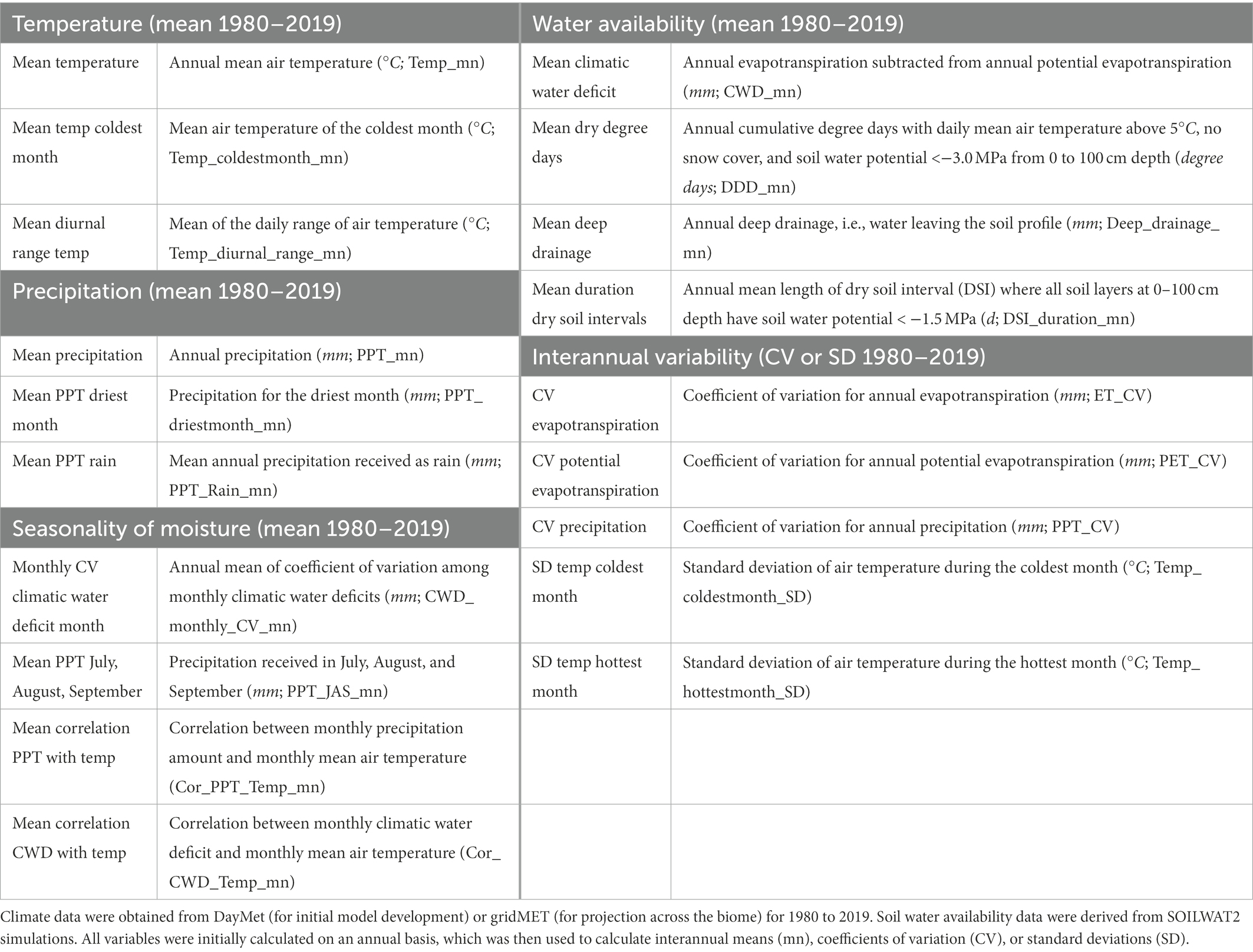
Table 1. Variables used in the analyses.

We randomly split the data set into a training/analysis set (0.70) and a test/assessment set (0.30), stratified by RSL and RST categories. Because of imbalanced sample sizes among RSL and RST categories, we performed synthetic minority over-sampling (i.e., SMOTE) so that all sample sizes were approximately equal (Chawla et al., 2002). We standardized the continuous abiotic variables to a mean of 0 and unit variance, and tuned a random forest model on the training data using the accuracy statistic estimated from 10-fold cross-validation to select an optimal number of randomly sampled variables as candidates at each split (i.e., “mtry” parameter). The resulting model was assessed by its performance in classifying the cross-validation set within ecoregions, and the final model fitted to the training data set. This final model was used to generate predicted RSL and RST indicators for all plots, and the classification performance was evaluated from test set results. The supervised classification was performed using “tidymodels,” “themis,” “caret,” and “randomForest” packages in R version 4.1.2 (R Core Team, 2021).

We evaluated differences in climate and soil water availability among RSL and RST categories by identifying the most important indicators of RSL and RST among the set of 19 variables. We used the Jenks natural breaks algorithm (Jenks and Caspall, 1971) to suggest five break points separating the distribution of the permutation-based mean decreases in accuracy (MDA) values. The influence of the different indicators on RSL and RST within the top groups as defined by the Jenks natural breaks were evaluated by examining the distributions of the raw data, accumulated local effect plots (Biecek, 2018), and 2-way partial dependence plots (Greenwell, 2017). The 2-way partial dependence plots showed the patterns of random forest predictions within each level of RSL and RST in response to changes in two indicator variables simultaneously and were used to explore interactions between variables.

Mapping the indicators and comparing the ecoregions

To develop maps of the RSL and RST categories, we first compiled the indicator variables from the random forest models across the ecoregions within the study area. The primary spatial units were derived from gNATSGO (USDA Natural Resources Conservation Service [USDA NRCS], 2020). Where large map unit polygons dominated a grid cell, we used spatial units that represented the intersections between the map unit polygons and the 4-km grid of gridMET (Abatzoglou, 2013). Indicator variables were determined as described above and used by the random forest model to predict both RSL and RST categories for each spatial unit.

To assess variation in RSL and RST across ecoregions, we summed the proportion of the area within each ecoregion occupied by each category of RSL and RST. We restricted our summaries to those portions of the ecoregions occupied by sagebrush and pinyon juniper ecosystems within the rangelands data layer (Reeves and Mitchell, 2011) and excluded portions of the ecoregions which fell outside of the sagebrush biome perimeter.

Results

Resilience and resistance indicator variables

The climate and soil water availability variables selected for inclusion in the random forest models showed large differences across the study area due to changes in temperature associated with latitude and elevation, changes in seasonality of precipitation across an east to west longitudinal gradient, and regional soils and topography (Figure 1; Supplementary Figure 2). The random forest models that were derived from these variables had relatively high multiclass accuracy (80% for RSL and 75% for RST) and predicted the rarer classes well (sensitivity = 78% for RSL and 75% for RST). However, the accuracy and sensitivity of the random forest predictions for the RSL and RST categories differed among ecoregions due to variation in numbers of ecological types, numbers of sample plots within types, and complexity of ecological types (Supplementary Figure 3; Supplementary Tables 3, 4). Despite this, the percentage of plots with correct predictions of RSL was 95 to 96% in all ecoregions except the Wyoming Basin, which had 92% correct. For RST the percentage of plots with correct predictions was 93 to 96% with 90% in the Wyoming Basin.

FIGURE 1

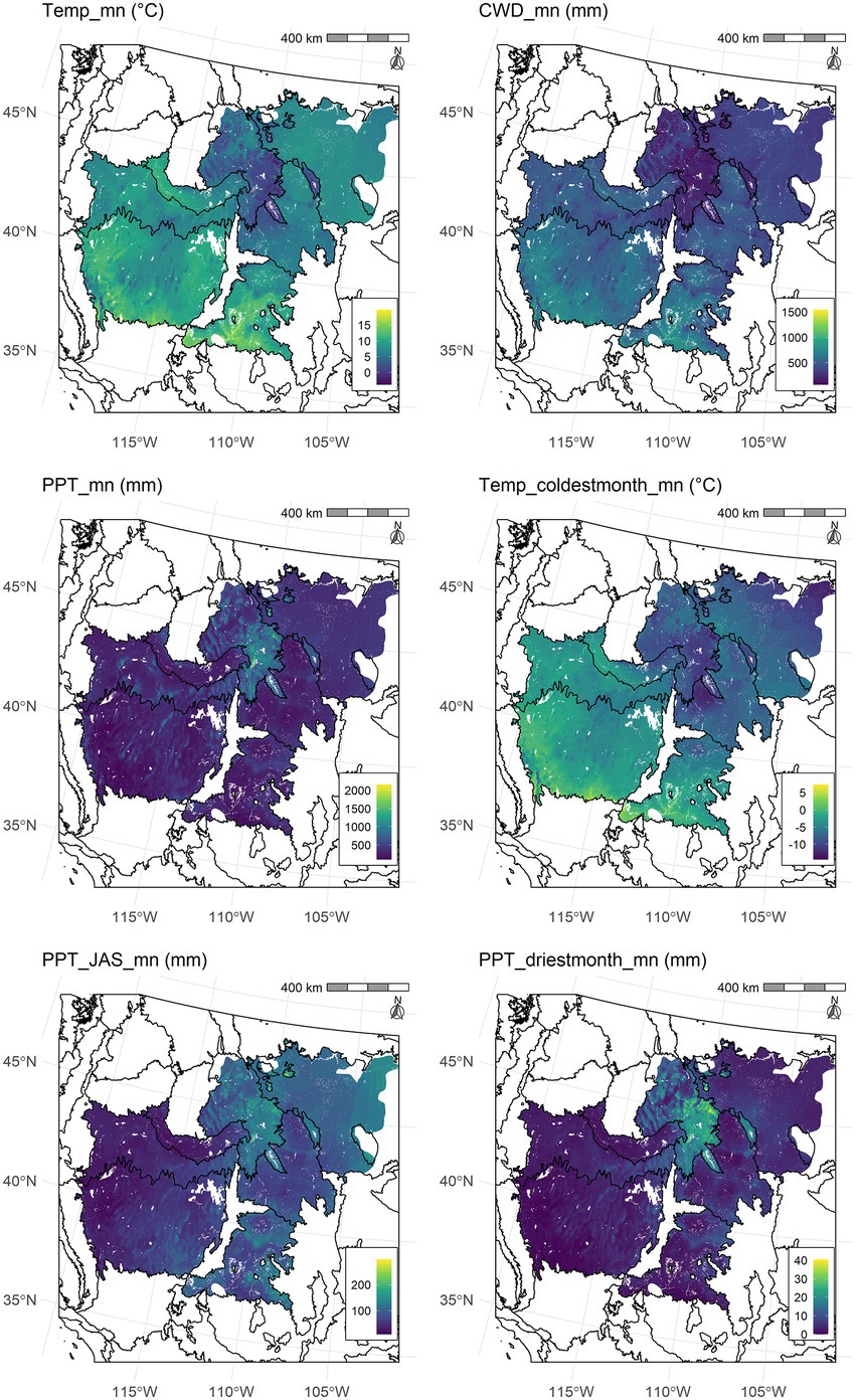
Figure 1. Maps of the most highly ranked predictor variables of resilience and resistance for the study area. Black lines indicate Level III EPA ecoregion boundaries (US Environmental Protection Agency [US EPA], 2022).

We derived five Jenks natural breaks for variable importance from the permutation-based mean decreases in accuracy (MDA) for RSL and RST. Variables in the first natural break for the RSL categories had MDAs ranging from 17.0 to 14.4% and were, in order of importance, mean temperature (Temp_mn) followed by climatic water deficit (CWD_mn) and mean precipitation (PPT_mn; Figure 2). The three variables in the second break had MDAs ranging from 11.8 to 9.8% and included coldest month temperature (Temp_coldestmonth_mn), summer precipitation (PPT_JAS_mn), and driest month precipitation (PPT_driestmonth_mn). Only one variable, Temp_mn, was in the first natural break for RST and its MDA was 14.6% (Figure 2). Variables in the second natural break for RST had MDAs ranging from 12.0 to 10.0% and were, in order of importance, PPT_JAS_mn, Temp_coldestmonth_mn, and CWD_mn. Variables in the third natural break had MDA values between 6 and 8.0% for both RSL and RST.

FIGURE 2

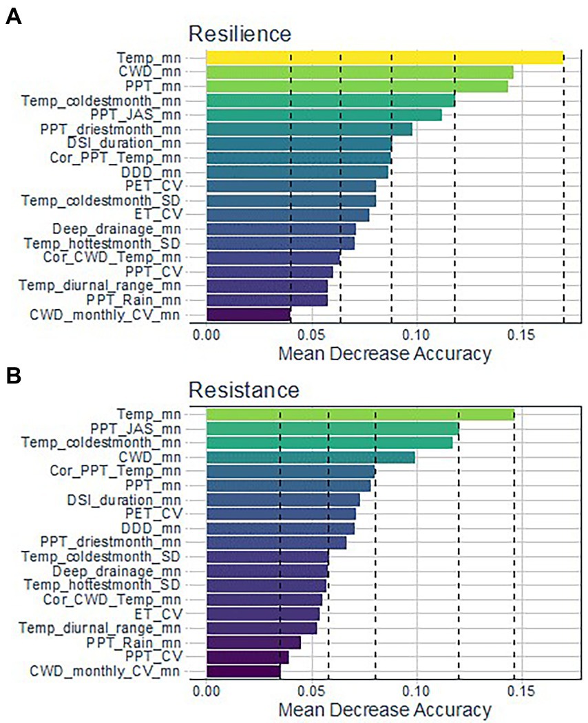
Figure 2. Climate and water availability variables ranked by permutation-based Mean Decrease in Accuracy (MDA) for the best random forest models of (A) resilience (overall model accuracy = 0.80, sensitivity = 0.78) and (B) resistance (accuracy = 0.75, sensitivity = 0.74) for the study area. Dashed lines indicate Jenks natural breaks dividing the set into five groups.

The predictor variables in the first two Jenks natural breaks generally exhibited distinct differences among the four RSL and RST categories and the categories showed clear separation in the random forest models (Figures 3, 4; Supplementary Figures 4, 5). Mean annual temperature (Temp_mn) was consistently important. RSL-H+MH had substantially lower Temp_mn than RSL-L (Figure 3). Temp_mn of RSL-M and RSL-ML were intermediate between RSL-H+MH and RSL-L and fairly similar. In the model, RSL-M and RSL-H+MH were separated from RSL-ML and especially RSL-L between Temp_mn of about 0 to 6°C. At about 7.5°C, RSL-L showed clear departure from the other categories. A progressive increase in CWD from RSL-H+MH to RSL-L existed and the four RSL categories had fairly unique values (Figure 3). In the model, all four categories were distinct from one another at CWD_mn below about 450 mm. At CWD_mn above about 700 mm, RSL-L separated from the other categories. Precipitation increased from RSL-L to RSL-H+MH and the four RSL categories had relatively distinct values of PPT_mn (Figure 3). RSL-L was distinct from the other categories below PPT_mn of about 375 mm. RSL-H+MH and M separated from one another and especially ML at close to 450 mm.

FIGURE 3

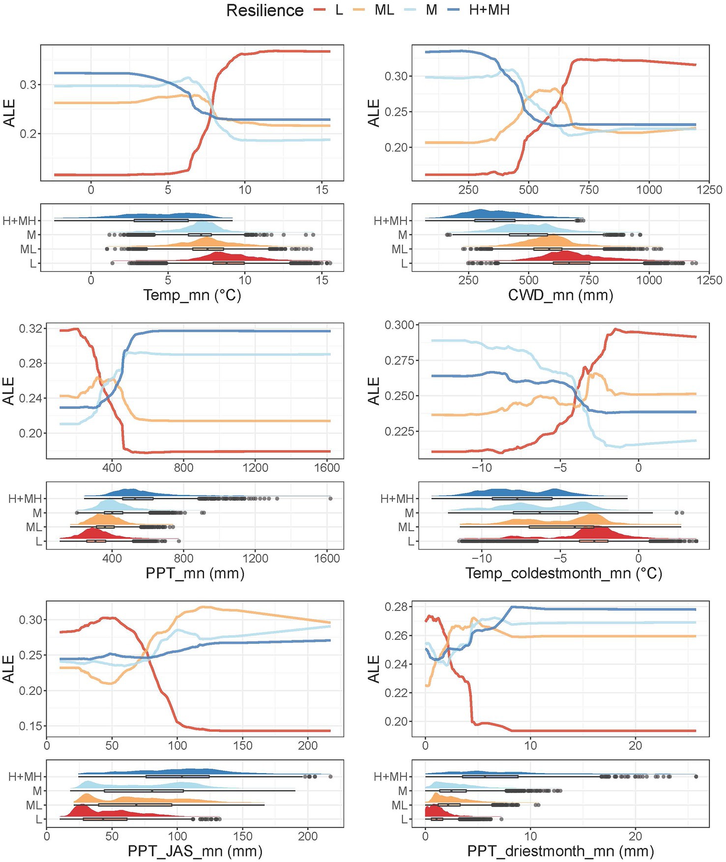
Figure 3. Accumulated local profile (ALE) plots and halfeye/box plots for the most highly ranked indictors of resilience. The ALE plots show effects of the focal variable on the random forest classification conditioned on the effects of other variables in the model. Halfeye/boxplots illustrate density of the raw data combined with a boxplot showing the median at the box’s center, the first and third quartiles (25th and 75th percentiles) as the box’s hinges, and whiskers extending to the largest and smallest values no further than 1.5 times the interquartile range from the hinge. Additional outliers are plotted as open circles.

FIGURE 4

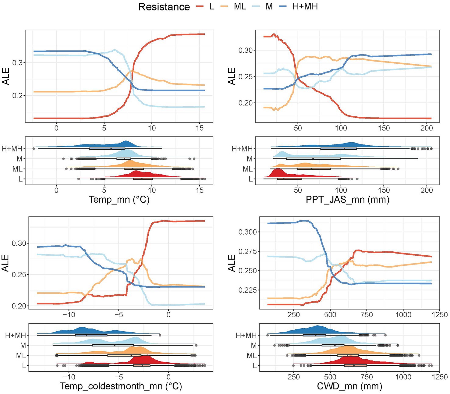
Figure 4. Accumulated local profile (ALE) plots and halfeye/box plots for the most highly ranked predictors of resistance. The ALE plots show effects of the focal variable on the random forest classification conditioned on the effects of other variables in the model. Halfeye/boxplots illustrate density of the raw data combined with a boxplot showing the median at the box’s center, the first and third quartiles (25th and 75th percentiles) as the box’s hinges, and whiskers extending to the largest and smallest values no further than 1.5 times the interquartile range from the hinge. Additional outliers are plotted as open circles.

The temperature of the coldest month was lower for RSL-H+MH than RSL-L and the values for the four categories were relatively distinct despite high variability (Figure 3). In the model, all four categories were clearly separated below Temp_coldestmonth_mn of about −4°C. Above −4°C, the categories became inverted and RSL-L and RSL-M showed clear departures from RSL-ML and RSL-H+MH. Summer precipitation was higher for RSL-H+MH than RSL-L and the RSL categories were relatively unique (Figure 3). A precipitation seasonality gradient occurred across the study area, and all four categories were highly variable. In the model, RSL-L separated clearly from the other categories at values of PPT_JAS_mn higher than about 75 mm. Precipitation during the driest month was higher for RSL-H+MH than RSL-L, although RSL-H+MH was highly variable (Figure 3). RSL-M and RSL-ML were intermediate between the other two categories but overlapped with one another. In the model, there was clear separation between RSL-L and the other categories between PPT_driestmonth_mn of about 2 and 5 mm.

Similar to RSL, RST-H+MH had lower temperatures than RST-L (Figure 4). However, Temp_mn of RST-ML and RST-M were more distinct. In the model, RST-M and RST-H+MH separated from RST-L at Temp_mn of about 7.5°C as for RSL. Summer precipitation was much lower for RST-L than for RST-H+MH and, although variable, was strongly skewed towards 0 mm. RST-M and RST-ML were intermediate between RST-L and RST-H+MH and also had high variability (Figure 4). In the model, RST-L and RST-ML were distinct from RST-M and RST-H+MH below PPT_JAS_mn of about 50 mm of precipitation. RST-ML was fairly distinct between PPT_JAS_mn of 50 and 100 mm, and RST-M and RST-H+MH split from RST-L at about 70 mm. Temperature during the coldest month increased from RSL-H+MH to RSL-L, but variability within the different categories was large (Figure 4). In the model, RST-L and RST-ML were distinct from RST-M and RST-H+MH below Temp_coldestmonth_mn of about −7.0°C. RST-L showed clear departure from the other categories at about −2.5°C. CWD also increased from RSL-H+MH to RSL-L (Figure 4). Clear separation of both RST-L and RST-ML from RST-M and RST-H+MH existed below CWD_mn of about 500 mm. At about 650 mm, RST-L separated from the other categories.

Relationships among indicator variables and resilience and resistance categories

The 2-way partial dependence plots showed the relationships among the highly ranked variables and helped illustrate the major characteristics of the categories. Additional climate and soil water availability variables that provided information about the RSL categories included the duration of dry soil intervals (DSI_duration_mn), correlation of temperature with precipitation (Cor_PPT_Temp_mn), and dry degree days (DDD_mn); those for RST included the monthly correlation between temperature and precipitation and mean precipitation (Figure 2). The predicted classification probabilities reflected the global averages for the study area, so the plotted probabilities for the RSL and RST categories with the fewest predictions had the lowest global averages and thus lower partial dependence plot probabilities.

In general, the characteristics of the resilience and resistance categories reflected the strong environmental gradients across the sagebrush biome. RSL-L was characterized by the highest mean temperatures and temperatures during the coldest month, while RSL-H+MH had the lowest mean temperatures and temperatures during the coldest month (Figure 5; Supplementary Table 5). RSL-L had large CWDs and not only low mean precipitation but also low precipitation during the driest month and in summer. In contrast, RSL-H+MH had low CWD and high mean precipitation as well as higher precipitation during the driest month and in summer. RSL-L was characterized by long dry soil intervals and high number of dry degree days, while RSL-H+MH exhibited the opposite characteristics (Supplementary Figure 6; Supplementary Table 5). RSL-ML and RSL-M had intermediate characteristics and followed the expected pattern, although RSL-M was more similar to RSL-ML than to RSL-H+MH (Figure 5; Supplementary Figure 6; Supplementary Table 5).

FIGURE 5

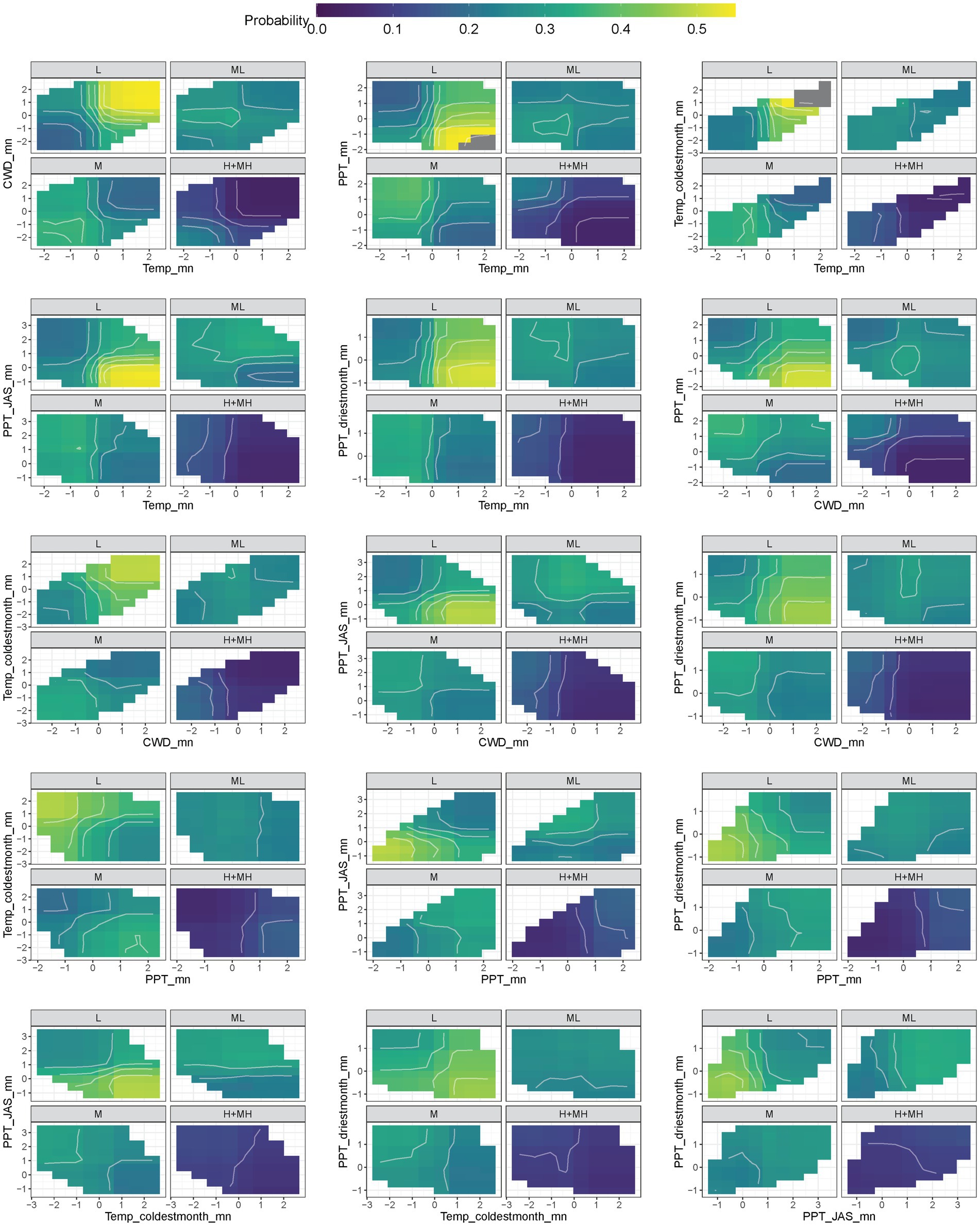
Figure 5. Two-way partial dependence plots (PDP) showing interactions between the six most highly ranked indicators for resilience. Lighter colors show higher probability of classification. Units for indicators are centered to a mean of 0 and scaled to unit variance.

RST-L was characterized by high mean temperatures, relatively high coldest month temperatures, and high CWDs, while RST-H+MH was characterized by low mean temperatures as well as very cold, coldest month temperatures, and the lowest CWDs (Figure 6; Supplementary Table 6). RST-L mean and summer precipitation were low, and correlations between temperature and precipitation were highly negative meaning that most precipitation fell in winter during the coldest time of year (Supplementary Figure 7; Supplementary Table 6). RST-H+MH had the highest overall precipitation and no consistent correlations between temperature and precipitation meaning that precipitation was equally likely to fall during all seasons (Supplementary Figure 7; Supplementary Table 6). Similar to RSL, RST-ML and RST-M had intermediate characteristics and followed the expected pattern (Figure 6; Supplementary Figure 7; Supplementary Table 6).

FIGURE 6

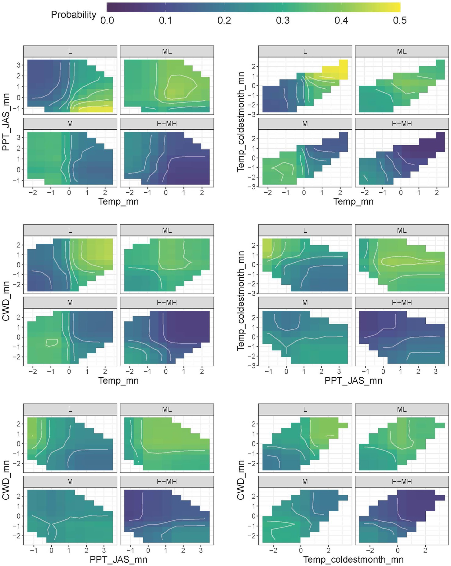
Figure 6. Two-way partial dependence plots (PDP) showing interactions between the four most highly ranked indicators for resilience. Lighter colors show higher probability of classification. Units for indicators are centered to mean of 0 and scaled to unit variance.

Variation in resilience and resistance categories across the study area

The differences in RSL and RST categories across the study area were illustrated well by maps created using the random forest models to predict the categories for polygons based on gNATSGO soil map units and gridMET grid cells (Figure 7). Because the study area encompassed the environmental gradients across the sagebrush biome, we were able to predict the RSL and RST categories for the entire biome (Supplementary Figure 8). The strength of the probabilities for low and high RSL and RST categories reflected their clear separation in the random forest models and the large differences in climate and soil water availability indicator variables (Supplementary Figure 9). Areas with abrupt boundaries between categories were due to differences in soil map unit component classifications among states or counties within states.

FIGURE 7

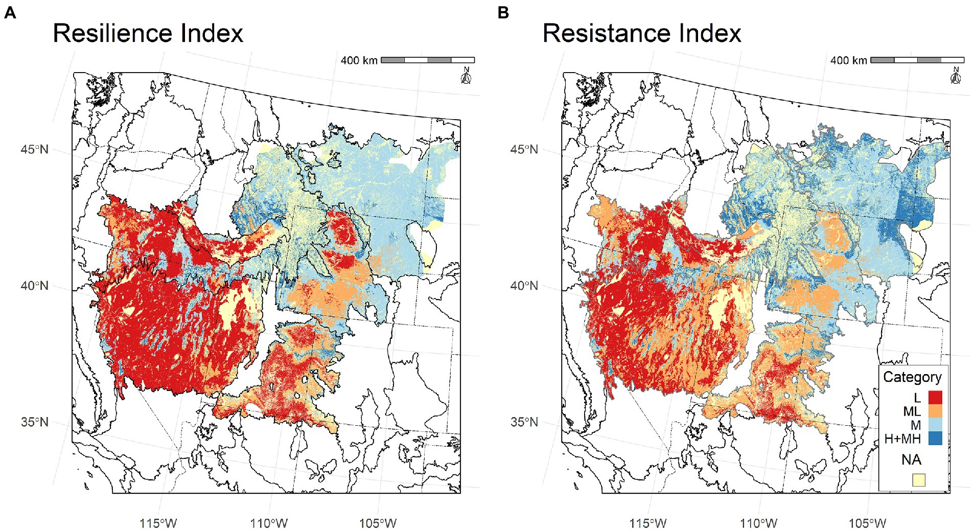
Figure 7. Maps of predicted (A) resilience and (B) resistance for the study area with Level III EPA ecoregions and states delineated (US Environmental Protection Agency [US EPA], 2022). Areas that do not support the focal ecosystems are shown in light yellow (“NA”).

The proportional areas of the RSL and RST categories differed among ecoregions (Figures 7, 8). Both RSL-L and RST-L occurred across large areas of the Northern Basin and Range+Snake River Plain, Central Basin and Range, and Colorado Plateau; RSL-L was also found in the north-central Wyoming Basin. These areas had the highest mean and warmest coldest month temperatures and lowest CWDs and summer precipitation (Figure 1). Larger areas of RSL-L than RST-L and conversely, smaller areas of RSL-ML than RST-ML, occurred in parts of the north-central Wyoming Basin, southeast Central Basin and Range and Colorado Plateau. This was likely because RST-ML was characterized by moderately high summer precipitation, which also occurred in areas of the Central Basin and Range, Colorado Plateau, and Wyoming Basin with RST-ML (Figure 1).

FIGURE 8

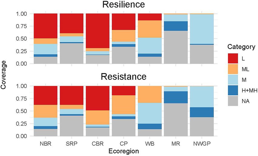
Figure 8. Proportion of total area in different resilience and resistance categories in each of the ecoregions. Portions of ecoregions that lie outside of the sagebrush biome are unclassified (“NA”). NBR, Northern Basin and Range; SRP, Snake River Plain; CBR, Central Basin and Range; CP, Colorado Plateau; WB, Wyoming Basin; MR, Middle Rockies; NWGP, Northwestern Great Plains.

RSL-M and RST-M covered the greatest areas in the Middle Rockies, Northern Basin and Range+Snake River Plain, and especially Wyoming Basin and Northwestern Great Plains (Figure 8). Areas with RSL-M and RST-M in the Middle Rockies and Northern Basin and Range+Snake River Plain were typically mountainous, while those in the Wyoming Basin and Northwestern Great Plains were characterized by high plains. All of these areas had moderately low mean and coldest month temperatures as well as moderately high CWDs and summer precipitation (Figure 1). RSL-M+MH and RST-M+MH occurred primarily in cold mountainous areas with high mean precipitation and low CWDs and covered the largest areas in the Middle Rockies with the Northwestern Great Plains a distant second.

Distinct patterns existed in the important indicator variables across the study area (Figure 1), and the indicator variables differed significantly between most ecoregions when analyzed by RSL and RST categories (Figures 9, 10). The RSL and RST categories typically had similar differences. An exception was the Middle Rockies, which had low sample sizes and high variability, especially for RSL-L and RST-L. The Northern Basin and Range+Snake River Plain had moderate temperatures and CWDs, high mean precipitation, but the lowest summer precipitation (Figures 9, 10). The Central Basin and Range had relatively high mean temperatures and CWDs across categories as well as relatively low summer and driest month precipitation. The Colorado Plateau had the warmest temperatures as well as low mean precipitation and high CWDs. The Colorado Plateau receives monsoonal precipitation and had the highest summer precipitation.

FIGURE 9

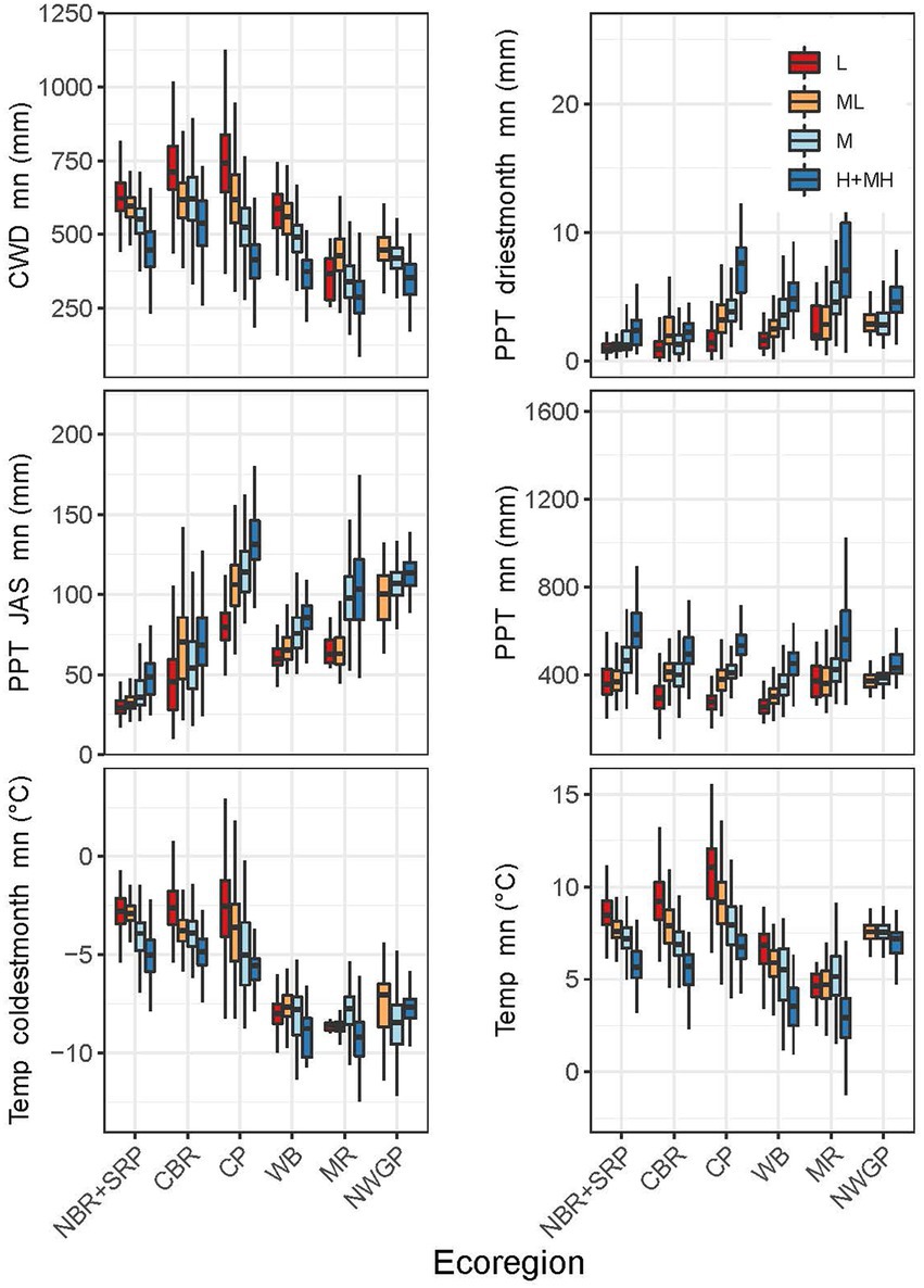
Figure 9. Boxplots for the most highly ranked predictor variables of resilience for each ecoregion by resilience category. Boxplot show the median at the box’s center, the first and third quartiles (25th and 75th percentiles) as the box’s hinges, and whiskers extending to the largest and smallest values. NBR, Northern Basin and Range; SRP, Snake River Plain; CBR, Central Basin and Range; CP, Colorado Plateau; WB, Wyoming Basin; MR, Middle Rockies; NWGP, Northwestern Great Plains.

FIGURE 10

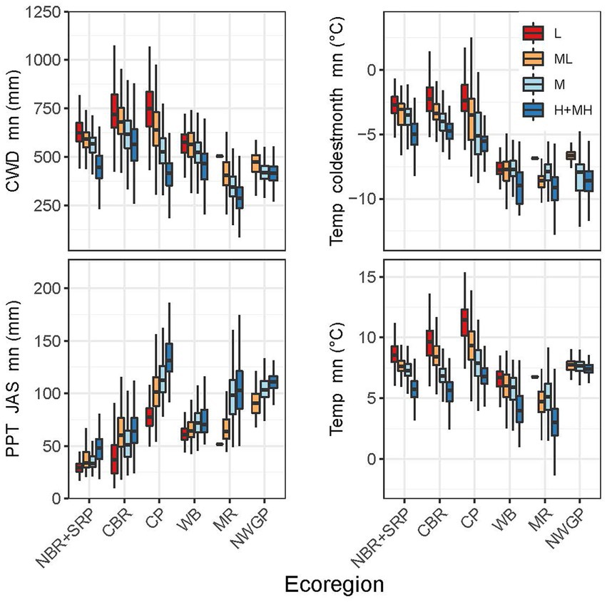
Figure 10. Boxplots for the most highly ranked predictor variables of resistance for each ecoregion by resistance category. Boxplot show the median at the box’s center, the first and third quartiles (25th and 75th percentiles) as the box’s hinges, and whiskers extending to the largest and smallest values. NBR, Northern Basin and Range; SRP, Snake River Plain; CBR, Central Basin and Range; CP, Colorado Plateau; WB, Wyoming Basin; MR, Middle Rockies; NWGP, Northwestern Great Plains.

The Wyoming Basin had among the coldest mean temperatures and lowest mean precipitation, but moderate summer and driest month precipitation and CWDs (Figures 9, 10). Coldest month’s temperature was consistently low across RSL and RST categories. RSL categories generally had larger differences than RST categories. The Middle Rockies had low mean and coldest month temperatures and the lowest CWDs. Mean precipitation was generally high and summer precipitation moderate. RSL and RST categories had similar differences. The Northwestern Great Plains lacked RSL-L and RST-L categories and had moderate mean temperatures, low coldest month temperatures, and relatively high summer and driest month precipitation. This ecoregion had the smallest differences among categories for all variables.

Discussion

We developed landscape-scale indicators of resilience to disturbance (RSL) and resistance to B. tectorum invasion (RST) for seven ecoregions that span the diverse environmental conditions in the sagebrush biome. To ensure applicability to management, our RSL and RST indicators were closely aligned with the U.S. National Cooperative Soil Survey (USDA Natural Resources Conservation Service [USDA NRCS], 2022c) data and Ecological Site Descriptions (USDA Natural Resources Conservation Service [USDA NRCS], 2022a) commonly used by managers to evaluate ecosystem recovery potential and determine appropriate management activities. To increase our ability to characterize RSL and RST in a rapidly changing environment, we used ecologically-relevant climate and water availability variables from ecohydrological simulations in our predictive models. The indicator variables that we derived differentiated both RSL and RST categories well and provided new insights into the important climate, water availability, and ecological drought metrics driving ecosystem recovery and annual grass invasions across the study area. The new indicators improve the ability to evaluate current levels of RSL and RST, project likely changes in a warming environment, and develop more effective prioritization schemes for the conservation and restoration of sagebrush ecosystems.

Resilience indicator variables and categories

Evaluating how indicators of RSL and RST vary across environmental gradients provides insights into the conditions that determine a system’s capacity to recover following disturbance and resist invasion by exotic species. The most highly ranked indicator variables in our RSL model, mean temperature, precipitation, and climatic water deficit, were a function of the strong environmental gradients that occur across the study area. These variables were similar to those that indicate RSL in dryland ecosystems both globally and regionally (Rigge et al., 2019; Yao et al., 2021). The second ranked indicator variables in the model, coldest month temperature, summer precipitation, and driest month precipitation, illustrated the influence of temperature regimes and precipitation seasonality on resilience and resistance within ecoregions. Ecoregions in the west and southeast (Northern Basin and Range+Snake River Plain, Central Basin and Range, Colorado Plateau) were warmer and drier across categories than those in the northeast (Middle Rockies, Northwestern Great Plains, Wyoming Basin). Particularly large differences existed among ecoregions in coldest month’s temperature. The differences among categories within ecoregions largely reflected the influence of topographic gradients. However, in the Northwestern Great Plains limited differences among RSL categories in all indicator variables helped explain the large contiguous areas of RSL-M and indicated that other variables, such as soil texture, were important in distinguishing among RSL categories.

Large gradients in seasonality of precipitation also exist across the study area, and these were reflected in the importance of summer and driest month’s precipitation in the models. Several studies indicate that areas receiving proportionately more precipitation in summer tend to be dominated by perennial grasses and show higher resilience to fire and other perturbations (Prevéy and Seastedt, 2014; Larson et al., 2017). We found that summer precipitation was positively related to resilience in all ecoregions, and across the study area, summer precipitation for RSL-L (43 mm) was less than half that for RSL-H+MH (103 mm). However, the RSL categories showed large differences in summer precipitation among ecoregions. The Colorado Plateau received the most summer precipitation across categories (RST-L = 79.8 mm and RST-H+MH = 131.2 mm), while the Northern Basin and Range+Snake River Plain received the least (RST-L = 29.5 mm and RST-H+MH = 48.8 mm). In all ecoregions, the importance of individual indicator variables in determining both RSL and RST categories were mediated by other highly ranked indicators. The differences in individual indicators like coldest month’s temperature and summer precipitation among ecoregions clearly illustrate the importance of evaluating the full set of climate and water availability variables likely to influence RSL and RST across landscapes as extensive and diverse as the sagebrush biome.

Important RSL indictor variables related to ecological drought were dry soil intervals and degree days (Chenoweth et al., 2022). The increase in frequency and severity of drought in recent decades is projected to intensify with warming temperatures (IPCC, 2022). Across the study area, length of dry soil intervals doubled from RSL-H+MH (14 days) to RSL-L (28 days), while number of dry degree days increased almost 4-fold from RSL-H+MH (346 days) to RSL-L (1,360 days). Warm and dry areas have the highest climate exposure (rate, magnitude, and nature of climate-induced stress). Areas with both high climate exposure and low ecological resilience are projected to have the greatest vulnerability to climate change (Comer et al., 2019).

Resistance indicator variables and categories

The top indicator variables for RST reflected those from distribution models and empirical studies, indicating the amount and seasonality of precipitation and winter temperature largely control resistance to B. tectorum. Three of these variables, climatic water deficit, coldest month’s temperature, and summer precipitation, were the top predictors for a study that used boosted regression trees and presence/absence data from >148,000 vegetation survey plots to evaluate the current and potential distribution of B. tectorum across the sagebrush biome (MacMahon et al., 2021). The best predictors for a study that used bioclimatic envelope modeling to evaluate the distribution of B. tectorum in the Northern Basin and Range, Snake River Plain, and Central Basin and Range were summer, annual, and spring precipitation followed by temperature during the coldest month (Bradley, 2009). In our RST model, the high ranking of mean temperature partly reflected use of soil temperature regimes in the derivation of our ecological types and subsequent RST rankings.

Strong empirical evidence links summer precipitation and coldest month’s temperature to RST. Our rankings of RST were based primarily on the fundamental niche of B. tectorum, which is constrained by environmental conditions, but also considered the realized niche, which is constrained by species interactions (Chambers et al., 2014a). Higher summer precipitation has been shown to increase RST largely because of increased native perennial grass dominance and higher levels of plant community competition with B. tectorum (Prevéy and Seastedt, 2014; Larson et al., 2017). Also, cold winter temperatures exceed the physiological tolerance of B. tectorum and limit germination, growth, or reproduction of the annual grass (Chambers et al., 2007; Bykova and Sage, 2012; Compagnoni and Adler, 2014). Similar to RSL, RST-L was characterized by high mean and coldest month’s temperatures, high climatic water deficit, and low summer and mean precipitation, while RST-H+MH was characterized by the opposite conditions. Larger areas of RST-ML than RSL-ML could be attributed primarily to the influence of summer precipitation for RST-ML in the Central Basin and Range and Colorado Plateau. The influence of coldest month’s temperature helped explain larger areas of RST-ML than RSL-ML in the Wyoming Basin and RST-H+MH in the Middle Rockies and Northwestern Great Plains.

In the western ecoregions higher RST, like higher RSL, can be attributed largely to lower temperatures, higher precipitation, and lower climatic water deficit at higher elevations (Chambers et al., 2014a). Progressive decreases in mean soil temperature and increases in late spring, fall, and October–June soil wet-days occur over the elevational gradients characterizing this area (Roundy and Chambers, 2021). Cooler temperatures and greater resource availability at higher elevations are associated with higher productivity, more competition from perennial native grasses, and greater biodiversity resulting in more resilient and resistant ecosystems (Bansal and Sheley, 2016; Wainwright et al., 2020).

Increases in coldest month’s temperature and climatic water deficit and decreases in summer precipitation are most likely to decrease RST in a warming environment. Recent increases in B. tectorum at higher elevations in the western ecoregions (Smith et al., 2021) are a function of increased climate suitability, more severe fire weather, and land management activities. Decreased RST is likely to be exacerbated by fires and management treatments that increase soil water availability (Roundy et al., 2020) and are located in areas without sufficient perennial native grasses to prevent competitive release of B. tectorum (Chambers et al., 2014b). However, in areas of the eastern ecoregions with both high summer precipitation and low coldest month’s temperatures, the magnitude of climate change may need to be relatively greater to result in significant changes in RST (Prevéy and Seastedt, 2014; Larson et al., 2017).

Relationship of resilience and resistance indicators to prior categorizations

We used Soil Survey (USDA Natural Resources Conservation Service [USDA NRCS], 2022c) and Ecological Site Description (USDA Natural Resources Conservation Service [USDA NRCS], 2022a) information as the basis for developing our larger-scale ecological types and RSL and RST categories. We used the indicator variables in our random forest models to predict the RSL and RST categories for the soil map unit polygons and develop our maps. Our previous work used soil climate regimes (soil temperature and moisture) mapped as part of the Soil Survey as a single index of both RSL and RST (Maestas et al., 2016; Chambers et al., 2017, 2019b). These static soil climate regimes were limited by inconsistencies in soil map units among states and counties within states and by conceptual definitions for moisture limitation that were not designed for ecological relevance or projections of the effects of long-term climate change (Bradford et al., 2019).

Our new RSL and RST indicators represent a significant advancement of our prior categorization of RSL and RST. The indicators were based on widely available climate data and new soil water availability metrics derived from process-based ecohydrological models that facilitate greater understanding of the effects of both climatic conditions and ecological drought on ecosystem recovery (Chenoweth et al., 2022). They allow the use of climate change modeling to project how RSL and RST are likely to change in a warming environment. And for the first time, separate RSL and RST indicators were developed that differentiate resilience to disturbances, like wildfire, and resistance to a major ecosystem transformer, the invasive annual grass, B. tectorum. Importantly, the new indicators do not negate efforts that used the initial index of RSL and RST (e.g., Chambers et al., 2017, 2019a,b; Crist et al., 2019; Rodhouse et al., 2021). Comparison of the soil temperature and moisture regimes with the new indicators illustrate the parallels and show that the new RSL and RST indices represent a refinement.

The approach for developing the new indicators was not without limitations. The use of experts to develop the ecological types and assign the RSL and RST categories may have influenced assignment of ecological sites to ecological types and of RSL and RST categories. Although the ecological site descriptions were developed using standard protocols, differences among states in the concepts used and information recorded also may have affected assignment of ecological sites to ecological types. Finally, by using soil map unit polygons to predict the RSL and RST categories, the differences in soil map units among states and counties within states were retained in the maps.

Resilience and resistance indicators as tools for prioritization

The new indicators increase the ability to evaluate relative RSL and RST across the diverse landscapes that characterize the sagebrush biome and to prioritize areas for conservation and restoration actions in those areas where they are likely to have the greatest benefits. The indicators provide a tool for assessing the likelihood of recovery following disturbances and management actions and risk of invasion and expansion of B. tectorum. They can be used in assessments of risks to remaining high-value ecosystems, including habitat for sagebrush-dependent species and National Parks and other conservation areas, and they provide useful information for prioritizing management actions (e.g., Ricca et al., 2018; Chambers et al., 2019a; Ricca and Coates, 2020; Rodhouse et al., 2021).

The new indicators can be used to update and refine frameworks for prioritizing sagebrush ecosystems for conservation and restoration actions based on RSL and RST (e.g., Ricca et al., 2018; Crist et al., 2019; Chambers et al., 2019b; Ricca and Coates, 2020; Rodhouse et al., 2021). In general, ecosystems with higher RSL and RST show less change after disturbances like wildfires, are less susceptible to invasion by B. tectorum, and recover more quickly than areas with relatively low RSL and RST (Chambers et al., 2014a,b, 2017). Also, areas with relatively large extents of intact native vegetation typically require less time to recover and lower amounts of intervention. Therefore, areas with higher RSL and RST as well as moderate to large extents of intact native vegetation often have the capacity to recover after disturbances like wildfires with minimal management intervention. These areas are a high priority for protective management strategies to maintain ecosystem connectivity as well as RSL and RST. Protective strategies may include reducing or eliminating disturbances from land uses and development, establishing conservation easements, practicing early detection and rapid response to invasives, and fire management (Crist et al., 2019).

Areas with moderate RSL and RST exhibit intermediate recovery potentials and susceptibility to B. tectorum (Chambers et al., 2019b). Priorities may include improving conditions through management activities such as identifying and correcting improper livestock grazing, reducing or eliminating new infestations of invasive plants, and restoring habitat (Crist et al., 2019). An emphasis on increasing perennial grasses and forbs can increase RST thus reducing the risk of altered fire regimes and transitions to invasive annuals.

Areas with relatively low RSL and RST and moderate to large extents of native vegetation are slower to recover from disturbances and have higher risk of B. tectorum invasions (Chambers et al., 2017). These areas often require substantial management intervention to decrease the risk of B. tectorum invasion and maintain or enhance ecological conditions after disturbance. Because these areas are at high risk of transitioning to alternative states dominated by invasive annuals, they also are often high priorities for protective management. Managers may decide to restore high-value resources in these areas, but the degree of difficulty and time frame required increase as RSL and RST decrease. In areas where climate change effects are projected to be severe, management actions may need to help ecosystems transition to new climatic regimes (Halofsky et al., 2019; Schuurman et al., 2022).

Regional risk assessments and planning efforts will be most effective if existing data layers, including the new indicators of RSL and RST, are considered along with projected climate change effects. Recent analyses of landscape change indicated that warmer and drier climatic conditions during the last three decades, as indicated by the average aridity index, caused a decrease in RSL across the dryland regions of China (Yao et al., 2021). In the sagebrush biome, higher temperatures during this same period were associated with declines in the cover of sagebrush, a keystone species and important indicator of RSL (Rigge et al., 2019). Temperature variables and climatic water deficit were important indicators of RSL and RST. Temperature explains a high proportion of the variability in soil water availability and ecological drought metrics for the western United States, including climatic water deficit and dry degree days (Chenoweth et al., 2022), and is more accurately predicted in climate change models than precipitation (IPCC, 2022). Climate change modeling could be used to project likely changes in the RSL and RST indicators. High to moderately high resilience and resistance are currently relatively rare, and although RSL and RST are likely to decrease with climate warming, variability in regional trends will undoubtedly occur. An understanding of the vulnerability of resources and likely success of management actions based on indicators of RSL and RST, and how they are likely to change in the future, can provide important information for assessing risks, prioritizing areas for management actions, and determining appropriate strategies.

Data availability statement

The datasets presented in this study can be found in online repositories. The name of the repository and accession number can be found here: https://datadryad.org/stash/dataset/doi:10.5061/dryad.h18931zpb.

Author contributions

JC led development and writing of the manuscript. JBro led database development and analyses. DS and JBra conducted the ecohydrological simulations and contributed to the analyses. All other authors contributed to various aspects of database development, analyses, and manuscript preparation. All authors contributed to the article and approved the submitted version.

Funding

This work was supported by the Joint Fire Sciences Program Project 19-2-02-11, and USDA Forest Service, Rocky Mountain Research Station.

Acknowledgments

The authors thank the USDA Natural Resources Conservation Service resource professionals who helped develop the ecological types and resilience and resistance rankings and Matt Reeves who modified the rangeland data layer. The manuscript was improved by review comments from Jeremy Maestas and Chelcy Miniat. The findings and conclusions in this publication are those of the authors and should not be considered to represent any official USDA or U.S. Government determination or policy. However, the findings and conclusions in this publication do represent the views of the U.S. Geological Survey.

Conflict of interest

The authors declare that the research was conducted in the absence of any commercial or financial relationships that could be construed as a potential conflict of interest.

Publisher’s note

All claims expressed in this article are solely those of the authors and do not necessarily represent those of their affiliated organizations, or those of the publisher, the editors and the reviewers. Any product that may be evaluated in this article, or claim that may be made by its manufacturer, is not guaranteed or endorsed by the publisher.

Supplementary material

The Supplementary material for this article can be found online at: https://www.frontiersin.org/articles/10.3389/fevo.2022.1009268/full#supplementary-material

References

Abatzoglou, J. T. (2013). Development of gridded surface meteorological data for ecological applications and modelling. Int. J. Climatol. 33, 121–131. doi: 10.1002/joc.3413

CrossRef Full Text | Google Scholar

Ainsworth, E. A., and Long, S. P. (2005). What have we learned from 15 years of free-air CO2 enrichment (FACE)? A meta-analytic review of the responses of photosynthesis, canopy properties and plant production to rising CO2. New Phytol. 165, 351–372. doi: 10.1111/j.1469-8137.2004.01224.x

PubMed Abstract | CrossRef Full Text | Google Scholar

Bansal, S., and Sheley, R. L. (2016). Annual grass invasion in sagebrush steppe: the relative importance of climate, soil properties and biotic interactions. Oecologia 181, 543–557. doi: 10.1007/s00442-016-3583-8

PubMed Abstract | CrossRef Full Text | Google Scholar

Bestelmeyer, B. T., Okin, G. S., Duniway, M. C., Archer, S. R., Sayre, N. F., Williamson, J. C., et al. (2015). Desertification, land use, and the transformation of global drylands. Front. Ecol. Environ. 13, 28–36. doi: 10.1890/140162

PubMed Abstract | CrossRef Full Text | Google Scholar

Biecek, P. (2018). DALEX: explainers for complex predictive models in R. J. Mach. Learn. Res. 19, 1–5.

Google Scholar

Bradford, J. B., and Lauenroth, W. K. (2006). Controls over invasion of Bromus tectorum: the importance of climate, soil, disturbance and seed availability. J. Veg. Sci. 17, 693–704. doi: 10.1658/1100-9233(2006)17[693:COIOBT]2.0.CO;2

CrossRef Full Text | Google Scholar

Bradford, J. B., Schlaepfer, D. R., Lauenroth, W. K., and Burke, I. C. (2014). Shifts in plant functional types have time-dependent and regionally variable impacts on dryland ecosystem water balance. J. Ecol. 102, 1408–1418. doi: 10.1111/1365-2745.12289

CrossRef Full Text | Google Scholar

Bradford, J. B., Schlaepfer, D. R., Lauenroth, W. K., Palmquist, K. A., Chambers, J. C., Maestas, J. D., et al. (2019). Climate-driven shifts in soil temperature and moisture regimes suggest opportunities to enhance assessments of dryland resilience and resistance. Front. Ecol. Evol. 7:358. doi: 10.3389/fevo.2019.00358

CrossRef Full Text | Google Scholar

Bradley, B. A. (2009). Regional analysis of the impacts of climate change on cheatgrass invasion shows potential risk and opportunity. Glob. Chang. Biol. 15, 196–208. doi: 10.1111/j.1365-2486.2008.01709.x

CrossRef Full Text | Google Scholar

Bradley, B. A., Curtis, C. A., Fusco, E. J., Abatzoglou, J. T., Balch, J. K., Dadashi, S., et al. (2018). Cheatgrass (Bromus tectorum) distribution in the intermountain Western United States and its relationship to fire frequency, seasonality, and ignitions. Biol. Invasions 20, 1493–1506. doi: 10.1007/s10530-017-1641-8

CrossRef Full Text | Google Scholar

Briske, D. D., Bestelmeyer, B. T., Stringham, T. K., and Shaver, P. L. (2008). Recommendations for development of resilience-based state-and-transition models. Rangel. Ecol. Manag. 61, 359–367. doi: 10.2111/07-051.1

CrossRef Full Text | Google Scholar

Brondizio, E. S., Settele, J., Díaz, S., and Ngo, H. T.. (eds.) (2019). Global assessment report on biodiversity and ecosystem Services of the Intergovernmental Science-Policy Platform on biodiversity and ecosystem services. Bonn, Germany: IPBES Secretariat.

Google Scholar

Brooks, M. L., Brown, C. S., Chambers, J. C., D’Antonio, C. M., Keeley, J. E., and Belnap, J. (2016). “Chapter 2. Exoctic annual Bromus invasions: comparisons among species and ecoregions in the Western United States” in Exotic Brome-Grasses in the Arid and Semiarid Ecosystems of the Western US. eds. M. J. Germino, J. C. Chambers, and C. S. Brown (New York, NY: Springer), 11–60.

Google Scholar

Burrell, A. L., Evans, J. P., and De Kauwe, M. G. (2020). Anthropogenic climate change has driven over 5 million km2 of drylands towards desertification. Nat. Commun. 11, 1–11. doi: 10.1038/s41467-020-17710-7

CrossRef Full Text | Google Scholar

Bykova, O., and Sage, R. F. (2012). Winter cold tolerance and the geographic range separation of Bromus tectorum and Bromus rubens, two severe invasive species in North America. Glob. Chang. Biol. 18, 3654–3663. doi: 10.1111/gcb.12003

CrossRef Full Text | Google Scholar

Chambers, J. C., Allen, C. R., and Cushman, S. A. (2019a). Operationalizing ecological resilience concepts for managing species and ecosystems at risk. Front. Ecol. Evol. 7:241. doi: 10.3389/fevo.2019.00241

CrossRef Full Text | Google Scholar

Chambers, J. C., Beck, J. L., Bradford, J. B., Bybee, J., Campbell, S., Carlson, J., et al. (2017). Science Framework for Conservation and Restoration of the Sagebrush Biome: Linking the Department of the Interior’s Integrated Rangeland Fire Management Strategy to Long-term Strategic Conservation Actions. Part 1. Science Basis and Applications. Gen. Tech. Rep. RMRS-GTR-360. Fort Collins, CO: U.S Department of Agriculture, Forest Service, Rocky Mountain Research Station. 213p.

Google Scholar

Chambers, J. C., Bradley, B. A., Brown, C. S., D’Antonio, C., Germino, M. J., Grace, J. B., et al. (2014a). Resilience to stress and disturbance, and resistance to Bromus tectorum L. invasion in cold desert shrublands of western North America. Ecosystems 17, 360–375. doi: 10.1007/s10021-013-9725-5

CrossRef Full Text | Google Scholar

Chambers, J. C., Brooks, M. L., Germino, M. J., Maestas, J. D., Board, D. I., Jones, M. O., et al. (2019b). Operationalizing resilience and resistance concepts to address invasive grass-fire cycles. Front. Ecol. Evol. 7:185. doi: 10.3389/fevo.2019.00185

CrossRef Full Text | Google Scholar

Chambers, J. C., Miller, R. F., Board, D. I., Pyke, D. A., Roundy, B. A., Grace, J. B., et al. (2014b). Resilience and resistance of sagebrush ecosystems: implications for state and transition models and management treatments. Rangel. Ecol. Manag. 67, 440–454. doi: 10.2111/REM-D-13-00074.1

CrossRef Full Text | Google Scholar

Chambers, J. C., Roundy, B. A., Blank, R. R., Meyer, S. E., and Whittaker, A. (2007). What makes Great Basin sagebrush ecosystems invasible by Bromus tectorum? Ecol. Monogr. 77, 117–145. doi: 10.1890/05-1991

PubMed Abstract | CrossRef Full Text | Google Scholar

Chawla, N. V., Bowyer, K. W., Hall, L. O., and Kegelmeyer, W. P. (2002). Smote: synthetic minority over-sampling technique. J. Artif. Intell. Res. 16, 321–357. doi: 10.1613/jair.953

PubMed Abstract | CrossRef Full Text | Google Scholar

Chenoweth, D. A., Schlaepfer, D. R., Chambers, J. C., Brown, J. L., Urza, A. K., Hanberry, B., et al. (2022). Ecologically relevant moisture and temperature metrics for assessing dryland ecosystem dynamics. Ecohydrology. 30:e2509.

Google Scholar

Comer, P. J., Hak, J. C., Reid, M. S., Auer, S. L., Schulz, K. A., Hamilton, H. H., et al. (2019). Habitat climate change vulnerability index applied to major vegetation types of the western interior United States. Land 8:108. doi: 10.3390/land8070108

CrossRef Full Text | Google Scholar

Compagnoni, A., and Adler, P. B. (2014). Warming, competition, and Bromus tectorum population growth across an elevation gradient. Ecosphere 5, 1–34. doi: 10.1890/ES14-00047.1

CrossRef Full Text | Google Scholar

Crist, M. R., Chambers, J. C., Phillips, S. L., Prentice, K. L., and Wiechman, L. A. (2019). Science Framework for Conservation and Restoration of the Sagebrush Biome: Linking the Department of the Interior’s Integrated Rangeland Fire Management Strategy to Long-term Strategic Conservation Actions. Part 2. Management Applications. Gen. Tech. Rep. RMRS-GTR-389. Fort Collins, CO: US Department of Agriculture, Forest Service, Rocky Mountain Research Station. 237p.

Google Scholar

D'Antonio, C. M., and Thomsen, M. (2004). Ecological resistance in theory and practice. Weed Technol. 18, 1572–1577. doi: 10.1614/0890-037X(2004)018[1572:ERITAP]2.0.CO;2

CrossRef Full Text | Google Scholar

Díaz, S., Settele, J., Brondízio, E. S., Ngo, H. T., Agard, J., Arneth, A., et al. (2019). Pervasive human-driven decline of life on earth points to the need for transformative change. Science 366, 1–10. doi: 10.1126/science.aax3100

PubMed Abstract | CrossRef Full Text | Google Scholar

Early, R., Bradley, B. A., Dukes, J. S., Lawler, J. J., Olden, J. D., Blumenthal, D. M., et al. (2016). Global threats from invasive alien species in the twenty-first century and national response capacities. Nat. Commun. 7, 1–9. doi: 10.1038/ncomms12485

CrossRef Full Text | Google Scholar

Greenwell, B. M. (2017). An R package for constructing partial dependence plots. R J. 9, 421–436. doi: 10.32614/RJ-2017-016

CrossRef Full Text | Google Scholar

Gremer, J. R., Andrews, C., Norris, J. R., Thomas, L. P., Munson, S. M., Duniway, M. C., et al. (2018). Increasing temperature seasonality may overwhelm shifts in soil moisture to favor shrub over grass dominance in Colorado plateau drylands. Oecologia 188, 1195–1207. doi: 10.1007/s00442-018-4282-4

PubMed Abstract | CrossRef Full Text | Google Scholar

Halofsky, J. E., Peterson, D. L., Ho, J. J., Little, N. J., and Joyce, L. A. eds. (2019). Climate change vulnerability and adaptation in the Intermountain Region [Part 2]. Gen. Tech. Rep. RMRS-GTR-375. Fort Collins, CO: U.S. Department of Agriculture, Forest Service, Rocky Mountain Research Station.

Google Scholar

Hanser, S. E., Leu, M., Knick, S. T., and Aldridge, C. L.. (2011). Sagebrush Ecosystem Conservation and Management: Ecoregional Assessment Tools and Models for the Wyoming Basins. Lawrence, KS: Allen Press.

Google Scholar

Hirota, M., Holmgren, M., Van Nes, E. H., and Scheffer, M. (2011). Global resilience of tropical forest and savanna to critical transitions. Science 334, 232–235. doi: 10.1126/science.1210657

PubMed Abstract | CrossRef Full Text | Google Scholar

Holling, C. S. (1973). Resilience and stability of ecological systems. Annu. Rev. Ecol. Syst. 4, 1–23. doi: 10.1146/annurev.es.04.110173.000245

PubMed Abstract | CrossRef Full Text | Google Scholar

IPCC (2022). Climate change 2022: Impacts, adaptation and vulnerability (Contribution of Working Group II to the Sixth Assessment Report of the Intergovernmental Panel on Climate Change).

Google Scholar

Jeffries, M. I., and Finn, S. P.. (2019). The sagebrush biome range extent, as derived from classified landsat imagery: U.S. Geological Survey data release.

Google Scholar

Jenks, G. F., and Caspall, F. C. (1971). Error on choroplethic maps: definition, measurement, reduction. Ann. Assoc. Am. Geogr. 61, 217–244. doi: 10.1111/j.1467-8306.1971.tb00779.x

CrossRef Full Text | Google Scholar

Knick, S. T., Hanser, S. E., Miller, R. F., Pyke, D. A., Wisdom, M. J., Finn, S. P., et al. (2011). “Chapter 12. Ecological influence and pathways of land use in sagebrush” in Greater Sage-Grouse. eds. S. T. Knick and J. W. Connelly (Berkely, CA: University of California Press), 203–252.

Google Scholar

Larson, C. D., Lehnhoff, E. A., and Rew, L. J. (2017). A warmer and drier climate in the northern sagebrush biome does not promote cheatgrass invasion or change its response to fire. Oecologia 185, 763–774. doi: 10.1007/s00442-017-3976-3

PubMed Abstract | CrossRef Full Text | Google Scholar

Lauenroth, W. K., Schlaepfer, D. R., and Bradford, J. B. (2014). Ecohydrology of dry regions: storage versus pulse soil water dynamics. Ecosystems 17, 1469–1479. doi: 10.1007/s10021-014-9808-y

CrossRef Full Text | Google Scholar

Levine, N. M., Zhang, K. E., Longo, M., Baccini, A., Phillips, O. L., Lewis, S. L., et al. (2016). Ecosystem heterogeneity determines the ecological resilience of the Amazon to climate change. Proc. Natl. Acad. Sci. U. S. A. 113, 793–797. doi: 10.1073/pnas.1511344112

PubMed Abstract | CrossRef Full Text | Google Scholar

MacMahon, D. E., Urza, A. K., Brown, J. A., Phelan, C., and Chambers, J. C. (2021). Modelling species distributions and environmental suitability highlights risk of plant invasions in western United States. Divers. Distrib. 27, 710–728. doi: 10.1111/ddi.13232

CrossRef Full Text | Google Scholar

Maestas, J. D., Campbell, S. B., Chambers, J. C., Pellant, M., and Miller, R. F. (2016). Tapping soil survey information for rapid assessment of sagebrush ecosystem resilience and resistance. Rangelands 38, 120–128. doi: 10.1016/j.rala.2016.02.002

CrossRef Full Text | Google Scholar

McColl, K. A., Roderick, M. L., Berg, A., and Scheff, J. (2022). The terrestrial water cycle in a warming world. Nat. Clim. Chang. 12, 604–606. doi: 10.1038/s41558-022-01412-7

CrossRef Full Text | Google Scholar

Miller, R. F., Knick, S. T., Pyke, D. A., Meinke, C. W., Hanser, S. E., Wisdom, M. J., et al. (2011). “Chapter 10. Characteristics of sagebrush habitats and limitations to Long-term conservation” in Greater Sage-Grouse. eds. S. T. Knick and J. W. Connelly (Berkeley, CA: University of California Press), 145–184.

Google Scholar

Nolan, C., Overpeck, J. T., Allen, J. R., Anderson, P. M., Betancourt, J. L., Binney, H. A., et al. (2018). Past and future global transformation of terrestrial ecosystems under climate change. Science 361, 920–923. doi: 10.1126/science.aan5360

PubMed Abstract | CrossRef Full Text | Google Scholar

O’Connor, R. C., Germino, M. J., Barnard, D. M., Andrews, C. M., Bradford, J. B., Pilliod, D. S., et al. (2020). Small-scale water deficits after wildfires create long-lasting ecological impacts. Environ. Res. Lett. 15:044001. doi: 10.1088/1748-9326/ab79e4

CrossRef Full Text | Google Scholar

Palmquist, K. A., Schlaepfer, D. R., Renne, R. R., Torbit, S. C., Doherty, K. E., Remington, T. E., et al. (2021). Divergent climate change effects on widespread dryland plant communities driven by climatic and ecohydrological gradients. Glob. Chang. Biol. 27, 5169–5185. doi: 10.1111/gcb.15776

PubMed Abstract | CrossRef Full Text | Google Scholar

Prevéy, J. S., and Seastedt, T. R. (2014). Seasonality of precipitation interacts with exotic species to alter composition and phenology of a semi-arid grassland. J. Ecol. 102, 1549–1561. doi: 10.1111/1365-2745.12320

CrossRef Full Text | Google Scholar

R Core Team (2021). R: A language and environment for statistical computing. R Foundation for Statistical Computing, Vienna, Austria. Available at: https://www.R-project.org/ (Accessed January 3, 2023).

Google Scholar

Reeves, M. C., and Mitchell, J. E. (2011). Extent of coterminous US rangelands: quantifying implications of differing agency perspectives. Rangel. Ecol. Manag. 64, 585–597. doi: 10.2111/REM-D-11-00035.1

CrossRef Full Text | Google Scholar

Renne, R. R., Schlaepfer, D. R., Palmquist, K. A., Bradford, J. B., Burke, I. C., and Lauenroth, W. K. (2019). Soil and stand structure explain shrub mortality patterns following global change–type drought and extreme precipitation. Ecology 100:e02889. doi: 10.1002/ecy.2889

PubMed Abstract | CrossRef Full Text | Google Scholar

Ricca, M. A., and Coates, P. S. (2020). Integrating ecosystem resilience and resistance into decision support tools for multi-scale population management of a sagebrush indicator species. Front. Ecol. Evol. 7:493. doi: 10.3389/fevo.2019.00493

CrossRef Full Text | Google Scholar

Ricca, M. A., Coates, P. S., Gustafson, K. B., Brussee, B. E., Chambers, J. C., Espinosa, S. P., et al. (2018). A conservation planning tool for greater Sage-grouse using indices of species distribution, resilience, and resistance. Ecol. Appl. 28, 878–896. doi: 10.1002/eap.1690

PubMed Abstract | CrossRef Full Text | Google Scholar

Richardson, D. M., and Gaertner, M. (2013). “Plant invasions as builders and shapers of novel ecosystems” in Novel Ecosystems: Intervening in the New Ecological World Order. eds. R. J. Hobbs, E. S. Higgs, and C. M. Hall (Chichester, UK: Wiley-Blackwell), 102–113.

Google Scholar

Rigge, M., Shi, H., Homer, C., Danielson, P., and Granneman, B. (2019). Long-term trajectories of fractional component change in the northern Great Basin, USA. Ecosphere 10:e02762. doi: 10.1002/ecs2.2762

CrossRef Full Text | Google Scholar

Rodhouse, T. J., Lonneker, J., Bowersock, L., Popp, D., Thompson, J. C., Dicus, G. H., et al. (2021). Resilience to fire and resistance to annual grass invasion in sagebrush ecosystems of US National Parks. Glob. Ecol. Conserv. 28:e01689. doi: 10.1016/j.gecco.2021.e01689

CrossRef Full Text | Google Scholar

Roundy, B. A., and Chambers, J. C. (2021). Effects of elevation and selective disturbance on soil climate and vegetation in big sagebrush communities. Ecosphere 12:e03377. doi: 10.1002/ecs2.3377

CrossRef Full Text | Google Scholar

Roundy, B. A., Miller, R. F., Tausch, R. J., Chambers, J. C., and Rau, B. M. (2020). Long-term effects of tree expansion and reduction on soil climate in a semiarid ecosystem. Ecosphere 11:e03241. doi: 10.1002/ecs2.3241

CrossRef Full Text | Google Scholar

Scheffer, M. (2009). Critical Transitions in Nature and society. Princeton, NJ: Princeton University Press.

Google Scholar

Schlaepfer, D. R., and Andrews, C. M. (2021). rSFSW2: Simulation Framework for SOILWAT2. R package version 4.3.1. Available at: https://github.com/DrylandEcology/rSFSW2 (Accessed January 3, 2023).

Google Scholar

Schlaepfer, D. R., Bradford, J. B., Lauenroth, W. K., and Shriver, R. K. (2021). Understanding the future of big sagebrush regeneration: challenges of projecting complex ecological processes. Ecosphere 12:e03695. doi: 10.1002/ecs2.3695

CrossRef Full Text | Google Scholar

Schlaepfer, D. R., and Murphy, R.. (2021). “rSOILWAT2: An Ecohydrological Ecosystem-Scale Water Balance Simulation Model.” R package version 5.0.1. Available at: https://github.com/DrylandEcology/rSOILWAT2 (Accessed January 3, 2023).

Google Scholar

Schuurman, G. W., Cole, D. N., Cravens, A. E., Covington, S., Crausbay, S. D., Hoffman, C. H., et al. (2022). Navigating ecological transformation: resist–accept–direct as a path to a new resource management paradigm. BioSci. 72, 16–29. doi: 10.1093/biosci/biab067

CrossRef Full Text | Google Scholar

Shriver, R. K., Andrews, C. M., Pilliod, D. S., Arkle, R. S., Welty, J. L., Germino, M. J., et al. (2018). Adapting management to a changing world: warm temperatures, dry soil, and interannual variability limit restoration success of a dominant woody shrub in temperate drylands. Glob. Chang. Biol. 24, 4972–4982. doi: 10.1111/gcb.14374

PubMed Abstract | CrossRef Full Text | Google Scholar

Smith, J. T., Allred, B. W., Boyd, C. S., Davies, K. W., Jones, M. O., Maestas, J. D., et al. (2021). The elevational ascent and spread of exotic annual grasslands in the Great Basin, USA. bio Rxiv.

Google Scholar

Stephenson, N. L. (1990). Climatic control of vegetation distribution: the role of the water balance. Am. Nat. 135, 649–670. doi: 10.1086/285067

PubMed Abstract | CrossRef Full Text | Google Scholar

Thornton, M. M., Shrestha, R., Wei, Y., Thornton, P. E., Kao, S., and Wilson, B. E.. (2020a). Daymet: Annual Climate Summaries on a 1-km Grid for North America, Version 4. ORNL DAAC, Oak Ridge, Tennessee, USA.

Google Scholar

Thornton, M. M., Shrestha, R., Wei, Y., Thornton, P. E., Kao, S., and Wilson, B. E.. (2020b). Daymet: Monthly Climate Summaries on a 1-km Grid for North America, Version 4. ORNL DAAC, Oak Ridge, Tennessee, USA.

Google Scholar

Tolvanen, A., and Aronson, J. (2016). Ecological restoration, ecosystem services, and land use: a European perspective. Ecol. Soc. 21:47

Google Scholar

US Environmental Protection Agency [US EPA] (2022). Level III and IV ecoregions of the continental United States. Available at: https://www.epa.gov/eco-research/level-iii-and-iv-ecoregions-continental-united-states

Google Scholar

USDA Natural Resources Conservation Service [USDA NRCS]. (2020). Gridded National Soil Survey Geographic (gNATSGO) database for the conterminous United States. Available at: https://nrcs.app.box.com/v/soils. (FY2020 July official release).

Google Scholar

USDA Natural Resources Conservation Service [USDA NRCS]. (2022a). Ecological Site Descriptions. Available at: https://www.nrcs.usda.gov/getting-assistance/ technical-assistance/ecological-sciences/ecologicalsitedescriptions (Accessed January 3, 2023).

Google Scholar

USDA Natural Resources Conservation Service [USDA NRCS]. (2022b). PLANTS database. Plant list of accepted nomenclature, taxonomy, and symbols. Available at: https://plants.usda.gov/home (Accessed January 3, 2023).

Google Scholar

USDA Natural Resources Conservation Service [USDA NRCS]. (2022c). Web soil survey. Available at: https://www.nrcs.usda.gov/wps/portal/nrcs/main/soils/survey/ (Accessed January 3, 2023).

Google Scholar

Wainwright, C. E., Davies, G. M., Dettweiler-Robinson, E., Dunwiddie, P. W., Wilderman, D., and Bakker, J. D. (2020). Methods for tracking sagebrush-steppe community trajectories and quantifying resilience in relation to disturbance and restoration. Restor. Ecol. 28, 115–126. doi: 10.1111/rec.13060

CrossRef Full Text | Google Scholar

Wiken, E., Jiménez Nava, F., and Griffith, G.. (2011). “North American Terrestrial Ecoregions—Level III.” Montreal, Canada: Commission for Environmental Cooperation.

Google Scholar

Williamson, M. A., Fleishman, E., Mac Nally, R. C., Chambers, J. C., Bradley, B. A., Dobkin, D. S., et al. (2020). Fire, livestock grazing, topography, and precipitation affect occurrence and prevalence of cheatgrass (Bromus tectorum) in the central Great Basin, USA. Biol. Invasions 22, 663–680. doi: 10.1007/s10530-019-02120-8

CrossRef Full Text | Google Scholar

Winthers, E., Fallon, D., Haglund, J., DeMeo, T., Nowacki, G., Tart, D., et al. (2005). Terrestrial Ecological Unit Inventory Technical Guide. Gen. Tech Rep. WO-68. Washington, D.C.: U.S. Forest Service, Ecosystem Management Coordination Staff, Washington Office.

Google Scholar

Yao, Y., Liu, Y., Wang, Y., and Fu, B. (2021). Greater increases in China's dryland ecosystem vulnerability in drier conditions than in wetter conditions. J. Environ. Manag. 291:112689. doi: 10.1016/j.jenvman.2021.112689

PubMed Abstract | CrossRef Full Text | Google Scholar

Young, D. J. N., Jeronimo, S. M. A., Churchill, D. J., Kane, V. R., and Latimer, A. M. (2021). The utility of climatic water balance for ecological inference depends on vegetation physiology assumptions. Glob. Ecol. Biogeogr. 30, 933–949. doi: 10.1111/geb.13277

CrossRef Full Text | Google Scholar

Zhang, W., Li, Y., Wu, X., Chen, Y., Chen, A., Schwalm, C. R., et al. (2021). Divergent response of vegetation growth to soil water availability in dry and wet periods over Central Asia. J. Geophys. Res. Biogeo. 126:e2020JG005912. doi: 10.1029/2020JG005912

CrossRef Full Text | Google Scholar